Some problems in ergodic theory

University of Warwick institutional repository:

http://go.warwick.ac.uk/wrap

A Thesis Submitted for the Degree of PhD at the University of Warwick

http://go.warwick.ac.uk/wrap/58569

This thesis is made available online and is protected by original copyright.

Please scroll down to view the document itself.

Some

Problems

In

Ergodic Theory

by Anthony Nicholas Quas

Mathematics Institute, University of Warwick,

Coventry, CV47AL.

Thesis submitted in partial fulfilment of the requirements of the degree of Doctor of

Philosophy at the University of Warwick

Table of Contents

Chapter 1. Invariant Measures for Families of Circle Maps

1·1 Introduction

1·2 Two exam ples showing necessi ty of some conditions for

Theorem 1·1

1·3 Proof of Theorem 1·1

Chapter 2. Expanding Maps, g-Measures and Generalized

Bak-er's Transformations

2·1 Introduction

2·2 Connections between g-Measures, Expanding Maps and

Generalized Baker's Transformations

2·3 Construction of Examples of Expanding Maps

2·4 Some Possible Approaches to Question 1

Chapter 3. Representation of Markov Chains on Manifolds

3·1 Introduction

3·2 Previously Known Results

3·3 Background for Smooth Representation

3·4 Physical Motivation for Theorem 3·3

3·5 Differential Equations Background for Theorem 3·3

3·6 Proof of Theorem 3·3

3·7 Invariant Measures for Smooth Markov Chains

Chapter 4. Representation of Markov Chains on Tori

4·1 Representation of Markov Chains on Tori

4·2 Degree of a Markov Chain on the Circle

4·3 A Markov Chain which cannot be Represented by

Table of Figures

Figure 1·1 Possible arrangement of intervals about a periodic point 6

Figure 1·2 Lift of an iterate of a circle map showing the types of 7

periodic points

Figure 1·3 A family for which the conclusion of the theorem fails 9

Figure 1·4 'Speed Function' for the counterexample 10

Figure 1·5 Typical diagram of periodic points against parameter 16

Figure 1·6 Possible arrangement of chosen periodic points 19

Figure 2·1 Possible graph of <P 34

Figure 2·2 Fundamental partition of Sunder Tf 34

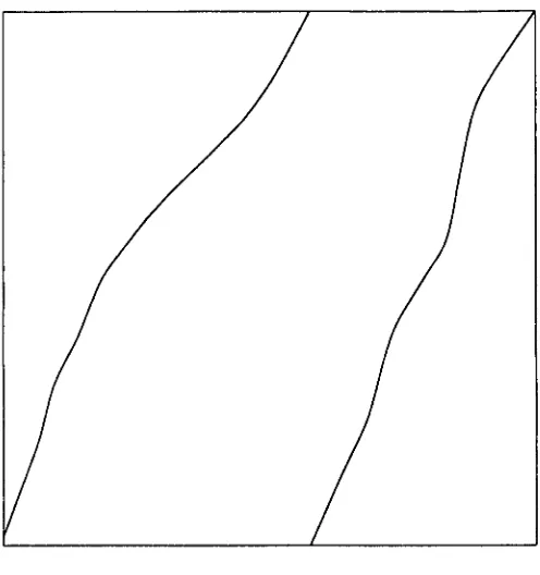
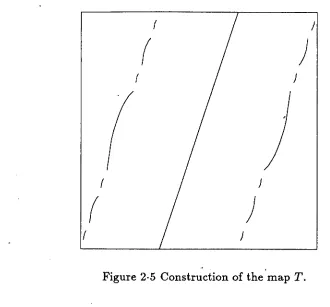
Figure 2·3 Graph of T 44

Figure 2·4 Configuration of J intervals 47

Figure 2·5 Construction of the map

T

47

Acknowledgements

I would like to thank my supervisor, Peter Walters, for the encouragement and help which he offered during the work for this thesis. Sebastian Van Strien was of assistance

in suggesting some of the questions which are addressed in Chapter 1. Thanks to Saul

Jacka and Chris Bose for interesting conversations about some of the questions raised in Chapter 2, and to Chris Bose for bringing to my attention his work on generalized baker's transformations. I would also to acknowledge useful conversations and advice from Mario Micallef, Janice Booth and Jim Eells during the preparation of Chapter 3.

Declaration

I declare that the work contained in this thesis is original, except where otherwise

indicated. In particular, Chapter 2 contains a survey of the known results about the

Summary

The thesis consists of a study of problems in ergodic theory relating to one-dimensional

dynamical systems, Markov chains and generalizations of Markov chains. It is divided

into chapters, three of which have appeared in the literature as papers. Chapter 1 looks at continuous families of circle maps and investigates conditions under which there is a weak*-continuous family of invariant measures. Sufficient conditions are exhibited and the necessity of these conditions is investigated. Chapter 2 is about expanding maps of the interval and the circle, and their relation with g-measures and generalized baker's trans-formations. The g-measures are generalizations of Markov chains to stochastic processes with infinite memory and generalized baker's transformations are geometric realizations of

these. The chapter is based around the question of whether there exist expanding maps

preserving Lebesgue measure, for which Lebesgue measure is not ergodic. Results are

known if the map is sufficiently differentiable (for example

C1+

Q), but the

Cl

case is still

unclear. The chapter contains some partial solutions to this question. Chapter 3 is about representation of Markov chains on compact manifolds by measured collections of smooth maps. Given a measured collection of maps, a Markov chain is induced in a natural fashion. This chapter is about reversing this process. Chapter 4 describes a specialization of the setting of Chapter 3 to Markov chains on tori. In this case, it is possible to demand more of the maps of the representation than smoothness. In particular, they can be chosen to be local diffeomorphisms. The chapter also addresses the question of whether in general the

maps can be taken to be diffeomorphisms and gives a counterexample showing that there

S01l1eProblems

in

Ergodic Theory

Anthony Quas

This dissertation concerns itself with problems of ergodic theory, the branch of

dy-namical systems theory which deals with problems of long-term averages of values of a

measurement taken at discrete intervals of time. In general, the formulation is that T is

a map from some measure space

X

to itself and

f

is an

L1

function

X

---+ R. The main

objects of study in ergodic theory are the averages

Ergodic theory gives conditions for these to converge pointwise almost everywhere with

respect to an appropriate measure (or in

L1)

to a function

1.

These measures are in fact

the invariant measures, which are central in the study of ergodic theory. Further conditions

can be given to ensure that the limit function

j

is constant almost everywhere with respect

to the invariant measure for any

L1

function

f.

This turns out to be extremely important.

Chapter 1 of this dissertation considers the case where there is a continuously

pa-rameterized family of circle maps (that is orientation-preserving_, homeomorphisms of the

circle). Each circle map is known to have at least one invariant measure. In this chapter,

I consider whether the invariant measures for the family of circle maps may be chosen to

vary continuously with respect to the parameter. In general, I show that subject to certain

conditions, this may be arranged by careful choice of the invariant measure. In an

experi

-mental situation, the invariant measure is determined by the initial conditions. Typically,

without special initial conditions, one would not expect to see continuous variations of the

thus show that while typically long-term averages change discontinuously with respect to

small changes in the parameter, they may in special circumstances vary continuously.

Chapter 2 deals with the relationships between the concepts of expanding maps,

9-measures and generalized baker's transformations. The starting point is the question of

uniqueness of absolutely continuous invariant measures for Cl expanding maps of the

interval and the circle. This leads naturally into an investigation of 9-measures, which

may be considered as a generalization of Markov chains to processes which depend on the

entire past, not just the last outcome. These are known to have a geometric realization

as generalized Baker's transformations. This realization is studied in Chapter 2 and made

more explicit. Finally, I present some examples of possible constructions of Cl maps which

might have more than one absolutely continuous invariant measure. Ifcorrect, these would

provide a solution to a question of Keane ([Kea)).

Chapter 3 looks at Markov chains on compact manifolds. Conditions are found for

Markov chains, under which there exists a family of smooth maps from the manifold to

itself and a probability measure on them such that applying the maps at random according

to the probabilities specified by the measure reproduces the Markov chain. This is called

a representation of a Markov chain. A representation of a Markov chain allows it to be

viewed as a Random Dynamical System (RDS), as described in [Ki] and [AC].

Chapter 4 is a specialization of Chapter 3 to the case where the manifold is a torus.

In this case, it is shown that a smooth Markov chain admits a representation by local

diffeomorphisms. It is then natural to ask whether such a Markov chain in fact admits a

representation by diffeomorphisms. It is shown that in general this is not the case.

Chapter

1.

Invariant Measures

for Families of Circle Maps

1.

Introduction

This chapter considers the invariant measures of a continuous family of circle maps.

There is some evidence (see below) that a continuous family of circle maps should have

a continuous family of invariant measures. In fact, this does not always turn out to be

the case, but in this chapter, we give conditions for the conclusion to hold and show the

necessity of some of these. The results of this chapter have appeared in the literature as

[Q2].

Let 7r denote the projection R ---+ SI given by x f-+ exp(27rix). We will denote in

the usual way intervals on the circle (for example, the interval

[a, b]

is the closed interval

starting at a and going anticlockwise round to

b).

By a circle map, we will always mean

an orientation-preserving homeomorphism

T :

SI -e+ SI. For a detailed introduction to

the theory of circle maps, the reader is referred to [CFS], §3·3. The main results, however,

,

are summarized below for convenience. The dynamical behaviour of circle maps is very

well understood, and may be principally characterized by the rotation number of the map.

This is a measure of the 'average rotation' that the map imparts to a point. To define

the rotation number of a circle map

T :

SI ---+ SI, we first need its lift

F :

R ---+ R. The

lift of a co"ntinuous map

rP

of the circle (not necessarily a circle map) is a continuous map

<I> : R---+ R defined by the equation 7r

0

<I> =

rP

0;'.

This is uniquely defined up to an additive

.

integer constant. The degree of the map

rP

is given by <I>( x

+

1) - <I>( x). This is always an

integer and is independent of the point

x

E

R

and the lift chosen. In the case of a circle

map, the degree is always 1. The rotation number of the circle map T is then given by

() li

Fn(x)-x

pT

=

m ,

Tt-OO n

where

F

is a lift of

T.

This limit exists for all z , and is independent of z , The convergence

of the limit is uniform in z and the rotation number is unique for a map Tup to an additive integer constant (depending on the particular lift chosen to represent

T).

The notion of a

circle map with rational rotation number is therefore well-defined, since this property does

not depend on the lift chosen. It can be shown that a circle map has rational rotation

number with denominator q say (with the fraction expressed in its lowest terms), if and

only if it has periodic points of period q. Further, if this is the case, then each point of the

circle converges monotonically to a periodic point under iteration of the map. From these

facts, it follows that a circle map with irrational rotation number has no periodic orbits.

Here, the dynamics are also well-understood: each point has the same w-limit point set

and this is either a Cantor set, or the whole circle. In the former case, the map is

semi-conjugate to a rotation through 211"times the rotation number, and in the latter case, the

map is conjugate to a rotation 'through 211"times the rotation number.

Itmay be shown by elementary means that the map taking a circle map to its rotation

number is continuous with respect to the CD-topology on the space of circle maps; see for

example [CFS], §3.3, theorem 2.

Suppose now that

F

is a lift of a circle map

T.

Write

R( x)

=

F( x) - x

and

r :

SI ---+

R;

y

1--+

R(1I"-I(y)).

This is well-defined since

R

is periodic, and is the amount of rotation

which the point y undergoes when it is acted upon by

T.

Now, we have

1Tt-I. 1

.~L

r

(T' (

11"(X ))) = ~ (

r:(

x) - x) .

From this it follows that ~

2:~:01

r(Ti(y))

converges uniformly to

p(T)

as

n

---7

00.

But, for

any invariant measure

v

for

T,

J

r(y) dv(y)

=

J ~

2:::01

r(Ti(y))

dv(y),

so taking limits,

we get

J

r(y) dv(y)

=

p(T).

This shows that the rotation number of a circle map is numerically equal to the amount

of rotation at each point integrated with respect to an invariant measure for the circle

map. As

T

changes continuously,

r(y)

and

p(T)

both change continuously. This suggests

the invariant measures also depend continuously on the circle map in some sense. The

appropriate sense of continuity turns out to be weak" -continuity, and this chapter contains

an investigation of the weak" -continuity of the invariant measures of circle maps.

In the statement of the theorems, we will need some definitions. We say that a family

(TCI')CI'EJ

of circle maps, with J a compact subinterval of R is a

continuous

family of circle

maps

ifthe map

T:

J X

SI

---7

S\

(a,e)

1-+

TQ'(e)

is continuous.

Given a circle map

T

with rotation number

p/q,

let

S

be the lift of

Tq

fixing the

preimages of the periodic points. Define

u(x)

=

S(x)-x.

Note that

u

satisfies the equation

u(x)

=

u(x

+

1), since the degree of

T"

is 1. The function

v: SI

---7 Rj

e

1-+

uCrr-l(e))

is then well-defined. Note that the zeros of v are precisely the periodic points of the map

T.

Then given a periodic point

e,

there may be a neighbourhood of

e

on which v takes

the value 0 only at

e

itself. Ifsuch a neighbourhood exists, we say the periodic point is of

definite type,

and conversely, if no such neighbourhood exists, we say the periodic point is

of

indefinite

type.

Ifthe periodic point is of definite type, it follows that there is an open

interval

II

clockwise from

e

with

e

as an endpoint on which. the sign of v is constant, and

[image:12.558.158.412.59.290.2]

"--I

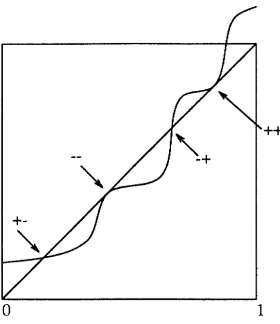
1

Figure 1·1 Possible arrangement of intervals about a periodic point.

We say that

e

is of type

++, +-, -+

or -- according to the sign of v on these

two intervals. A hyperbolic periodic point is one of type

+-

or

-+

(these are stable and

unstable respectiv~ly). The types

++

and -- of periodic point are non-hyperbolic and

have stability on one side only. We call a map with non-hyperbolic periodic points (or

sometimes its parameter value) critical. Note that if a point on a periodic orbit is of a

particular type, then all the other points on the orbit are of that type (this follows since

the maps are orientation-preserving homeomorphisms), so that it makes sense to say that

a periodic orbit is of a specific type, or in particular hyperbolic or non-hyperbolic (see

++

[image:13.558.176.378.54.288.2]

o

1

Figure 1·2 Lift of an iterate of a circle map showing the types of periodic points.

An invariant Borel probability measure (or briefly invariant measure) for a circle map

T

is a probability measure

f..£

on the Borel er-algebra

n

satisfying

f..£(T-

1

(B))

=

f..£(B)

for

any Borel set B. A circle map T is uniquely ergodic if it has exactly one invariant measure.

There is a well-known theorem of ergodic theory (see [Wa3], theorem 6·18) saying that if

T

is a circle map with irrational rotation number, then

T

is uniquely ergodic. A map with

rational rotation number is uniquely ergodic if and only if it has a unique periodic orbit

(see Lemma 2).

We are now ready to state the theorem:

Theorem 1. '

Suppose that (Ta )aEJ is

a

continuous

family of

circle

maps

such that

(i)

for each non-trivial interval K

on

which the rotation

number

has

a

constant value,

there

are

at most finitely

many

values

of a

in K for which Ta is critical,

and

hyperbolic.

Then there is a weak*-continuously varying family of probability measures

J.La

such that

J.La

is an invariant measure for

Ta.

Part of Theorem 1 was previously known to Herman. In particular, Herman showed

that the map taking a circle map with irrational rotation number to its unique invariant

probability measure is weak*-continuous on the sets

Fp,

the collection of circle maps with

rotation number equal to p (irrational). He in fact shows (see [He], proposition X.6.1), that

the (semi- )conjugacy h conjugating a circle map

f

E

Fp

to the rotation by 27rp depends

continuously on

f.

Since the invariant measure is given by

J.L(A)

=

A(h(A)),

this implies

that the map taking

f

to its invariant measure

J.L

is weak* -continuous when restricted to

Fp.

This result can easily be recovered from the proof here.

2. Two examples showing necessity of some conditions for Theorem 1

Before embarking on a proof of Theorem 1, we first present two examples to show that

some restrictions are necessary for the conclusions of the theorem to hold. In particular,

..

we exhibit families which do not satisfy condition (ii) for which the conclusion fails. It

seems likely that condition (i) is unnecessary for the conclusion of the theorem to hold,

although any significant relaxation of this condition will necessarily make the construction

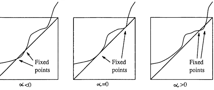
~Fixed

points points

0<,=0

[image:15.558.68.491.60.238.2]

Fixed points

Figure 1·3 A family for which the conclusion of the theorem fails.

The first example for which the conclusion fails is illustrated graphically in Figure 1·3.

The process which takes place is that a pair of fixed points vanish simultaneously with the

birth of another pair of fixed points. The limits from the two sides in the parameter space

of the invariant measures are concentrated on the dying pair (respectively new pair) for

parameter values lower than (respectively greater than) the critical value (see Lemma 2).

The example shows that even in the one-dimensional case, there exist examples for

which the unrestricted version of this theorem fails. The reliance of this proof on properties

of circle maps suggests that this would fail more spectacularly in higher dimensions.

This example works by having a parameter value such that the probability measures

for parameters on the left converge to a limit and similarly with parameters on the right,

but that the two limits fail to agree. It is then natural to ask if this is the only way that

the theorem .could go wrong. In particular, if a parameter value is on the boundary of an

interval on which the rotation number is rational, then this construction cannot be used.

The question is then whether the condition (ii) needs to apply at the boundary of regions

The next example, which is more complicated, shows that the conclusion of the

the-orem need not hold even if condition (ii) fails only on the boundary of an interval in the

parameter space on which the rotation number is constant. To write down the example,

we regard the circle as the interval [0,1) mod 1. The maps which we consider are then of

the form

T( x)

=

z

+

v( x)

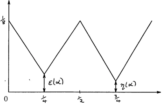
mod 1. The form of the functions V which we are considering is

[image:16.564.140.419.245.424.2]

shown in Figure 1·4.

Figure 1·4 'Speed Function' for the counterexample.

The function V depends on the parameters € and TJ. It is ,clear that if € and TJ are

allowed to vary continuously with respect to a parameter a say, then the family of circle

maps given by

TO'(x)

=

x +vO'(x)

mod 1 is in fact a continuous family of circle maps. The

family VO' is given explicitly by the expression

x

E [O,~]

XE[~,l]·

We then consider a family with the properties that

€(

a) ~

0 and TJ(

a) ~

0 as

a ~ ao,

and investigate the limit of the invariant measures of the maps TO'as

a ~ ao

and

as a -t ao. In this case, the limit is a measure

J.L

concentrated at the points

i

and ~ with

(1)

It is clear that there exist examples of continuous functions

t:(

a) and 1](a) with the

properties that t:(a) -t 0 and 1](a) -t 0 as a -t ao, t:(a)

>

0 and 1](a)

>

0 for all a

<

ao

such that the limit of log

t:/

log1]fails to exist as a -t ao.

It is a well-known fact of ergodic theory that each circle map

TC'<

has some invariant

measure, J.LQ say (see [Wa3], corollary 6.9.1). To evaluate the limiting measure

J.L

described

above, we take a small set containing

i,

say A =

[i -

h,

i

+

h) and a similar one containing

i,

say

B

=

[i -

h,

i

+

h),

and estimate

J.LQ(A)

and

J.LC'«B)

for a -e+ ao. To do this, we note

that if it takes between nand n

+

1 steps 'for a point to go all the way around the circle'

(that is if 0 ~

TQ~l+l(O)

<

TC'«O)

and this is the first such

n),

and if it takes between m

and m

+

1 steps for a point to go through

A

(that is, if TQm+l

(i -

h) ~

i

+

S

and this is

the smallest such m), then

where XA is the characteristic function of the set A. This follows by invariance of the measure. But for each point, we have

n-l

m-I 1", . m+l

--~-~XAoTQ'(:Z:)~ ,

n n . n

1=0

It follows that

IJ.LQ(A) -

7~

I ~ ~.

There is of course a similar result for

J.LQ(B).

Ifwe then

show that the amount of steps in each cycle spent outside sets

A

and

B

is bounded above

by some constant, then it is clear that we can evaluate the limit of

J.LQ(A)

as a -t ao,

calculation which we need to perform is to solve a simple recurrence relation to estimate

the time spent in certain sets of a very simple form. Suppose then we are considering

a set

C

of the form

[O,a)

and the 'speed' function is given by

v(x)

=

c - (c -

b)x/a

where c -

b

<

a,

and we have

T(x)

= X +

v(x)j

then the recurrence relation is Xn+l

=

c + (1 - (c -

b)/a)x

n. Let

p

=

1 - (c -

b)/a.

Then we are solving Xn+l

=

C +

px

n. The

solutions are Xn

=

c/(1 -

p) + Apn. By substituting the initial conditions, we see that

in fact Xn =

c(1-

pn)/(1_

p).

The number of steps thus spent in the set

C

is thus the

rounded-up value of

log(1 - (1-

p)a/c)/logp

=

(logb/c)/logp.

We can now apply this to the collection of circle maps described above. In what follows,

we will require € and 7] to be bounded above by

/6.

The first thing we show is that the

amount of steps per cycle spent outside the sets

A

and

B

is bounded above by a constant

as € and 7]tend to zero. To show this, we note the symmetry of the situation: the number

of steps taken to get from

°

to

i -

b is the same as the number of steps to get from

±

+ 6 to ~. This number is given by the round up of log(8.

v(i -

6))/log(~ + 4€). This ,

is bounded above by log( 48)/ log( ~), so we see that the number of steps spent outside

A

and

B

is bounded above by 410g(48)/log(i). The number of steps in

A

is given by

-210g€/logO + 4€) plus a term which is bounded, and similarly the number of steps in

B

is given by -210g7]/logO +47]) plus a bounded term. Set

m(€)

= -210g€/logO +4€)

and

p(

7])

= ~

210g 7]/ logO + 47]). Then given a constant (J'

>

0, there exists a T such that

By elementary analysis, we see that the assertion of equation (1) is now proved, and thus

3. Proof of Theorem 1

A useful lemma is the following:

Lemma 2.

The invariant Borel

probability measures for a

circle

map

T with

rational

rotation

number

p/q

are

precisely those

measures

which

can be

expressed in the

form

q-l

1~ .

IL(A)

= -

L.J

v(T-Z

A),

q i=O

where v is

a probability measure concentrated on

the fixed points

of

T",

Proof. Certainly any Borel probability measure of the form described is invariant for the

circle map in question. Conversely, in the preliminary discussion, it was noted that each

point of the circle converges monotonically under iteration of the map to a periodic orbit.

From this, it follo~s that the only non-wandering points of the map are the periodic points.

There is then a standard theorem telling us the non-wandering set has full measure (that

is measure

1)

with respect to any invariant Borel probability measure (see [Wa3], theorem

6·15). The remainder of the proof follows easily from the invariance of the measure.

Lemma 3.

Suppose that (Ta )aEJ is

a

continuous family

of

circle maps such that Tao

has a

hyperbolic periodic orbit

of

period q through

a

point

e

E SI.

Then

for each

neighbourhood

M

of

e,

there exists

a

neighbourhood

N of ao

such that

if (3 E N,

then Tf3has

a

periodic

point

of

period q in M.

Proof. Suppose that we are given a neighbourhood M of

e.

Then there must exist a

closed subinterval

1

of

M

with

e

E Int(l) with the property that

Tao q(l)

C Int(l) or

Tao

q(Int(l)) ::::>

(1)

according to whether

e

is stable or unstable. But then for any

T

which

or

Tq(Int(I))

:) I

respectively). But then it follows by Brouwer's fixed point theorem that

T has a periodic point of period q in Int(I).

Lemma 4.

Suppose X is

a compact

metric

space and To :

X

-+

X is

a

continuous

map

which is uniquely

ergodic,

with unique invariant

measure Vo, say.

Then for

any

weak*-neighbourhood N

of Vo,

there is

a

neighbourhood U

of To

such that for

T E

U

and v any

invariant

measure

for T,

we have

v

E

N.

Proof. By reducing N if necessary, we may first of all assume that N is a basic neighbour-hood of Vo (that is N

=

{J.L :

I

J

fi dJ.L -

J

Ii

dvol

<

Ei, i

=

1, ...

,n}

for a finite sequence

Ui)l<i<n

of continuous functions and

(Edl<i<n

a finite sequence of positive bounds). We

-

-

-

-may further assume that n

=

1 as for larger n, we may simply take the intersections of the

resulting neighbourhoods

U

obtained from the proof below. We will therefore assume for

this proof that the neighbourhood

N

is given by

N

=

{J.L :

J

f

dj.£ -

J

f

dVQ

I

<

E}.

Now

assume for a contradiction that for any neighbourhood U of To, there is a map T E U

and an invariant measure v for T such that

I

J

f

dv -

J

f

dVQ

I

2:

E. It follows that there

exists a sequence of maps (Tn)nEN converging uniformly to To, having invariant measures

(2)

Since X is a compact metric space, the space of Borel probability measures on X is weak*-compact, hence weak*-sequentially compact. The sequence of measures

(v

n) therefore has

a convergent subsequence, (vn;) converging to j.£, say. Since vn; is invariant for Tn;, we

have for any continuous g, that

J

9 0

r;

dvn;

=

J

9 dvn;,

Vi.

(3)

Now since

Tn;

converges to

To

uniformly, it follows that

goTn;

converges to

goTo

uniformly,

and hence, taking limits of (3) asi -+ 00, we see that

J

goTo dJ.L

=

J

9 dJ.L

for any continuous

function

g.

It follows that

J.L

is an invariant measure for

To,

yet taking the same limit in

(2), we see that

J.L

=1=

va.

This contradicts our assumption that

To

was uniquely ergodic, and hence proves the Lemma. 0

We now proceed to the proof of Theorem 1.

Proof of Theorem 1.

Set C

=

CI{o:

E J :

p(Ta)

¢

Q}.

We will show that for those values of 0: in C, the

map

Ta

is uniquely ergodic. If

p(Ta)

¢

Q, then this is a standard ergodic theorem as noted

earlier. If

Ta

has a hyperbolic periodic point, of period q say, then by Lemma 3, there is a neighbourhood of parameter values about 0:, such that for maps with parameters in the

neighbourhood, there is a periodic point, and hence the rotation number is rational on a

whole neighbourhood of parameter values about 0:. In particular, 0:

¢

C. It follows that

if 0: E C and

p(Ta)

E

Q

then

Ta

has no hyperbolic periodic points. We therefore see that

Ta

must have periodic points, and these must all be non-hyperbolic. By hypothesis (ii) of

the theorem, we have that

Ta

has a unique periodic orbit. It now follows from Lemma 2,

that there is a unique invariant probability measure.

We proceed by defining

J.La

for 0: E

J\C.

First, note that since C is a closed set, we

have that J\C is an open subset of J and hence consists of a countable disjoint union of Open subintervals of J, say J1,J2, • ... Now fix such an interval Jj• Unless J, is one of

the end intervals, J, is open in R, so we write

J;

=

(O:j,f3j).

In this case,

Ta;

and

Tj3;

are uniquely ergodic, so the invariant measures are determined at the endpoints of the interval.

other. Now set K,

=

CI(Ji)

=

[ai,,Bi].

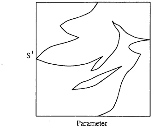
The idea behind the construction is as follows. Plotting the periodic points of

Ta

against

a

for

a

E

K,

gives a graph similar to Figure 1·5.

The invariant measure, being concentrated on the periodic points, must be chosen to be a

superposition of 'b-measures', moving along the periodic point curves. Since these curves

can terminate, it may be necessary to transfer to a new periodic curve. This must also

be done continuously, so in the construction, one curve is being phased in, while another

curve is being phased out.

SI

[image:22.549.137.390.258.464.2]

Parameter

Figure 1·5 Typical diagram of periodic points against parameter.

We construct an open cover for

Ki.

Suppose the rotation number of the maps with

parameters in

Ki

isp!q. This may be assumed by the continuity ofp. Then let

Sa

be a lift

of

Ta

q fixing the preimages (under

11")

of the periodic points, and set

ua(x)

=

Sa(x) -

z ,

Clearly the maps

(a,x)

H

Sa(x)

and

(a,a:)

H

ua(a:)

are continuous on

K,

X R. Given

a E

Ki ;

we seek a connected open neighbourhood Na containing a, and a continuous map

cPa :

CI(

N

a)

--+ R taking each parameter value to a fixed point of

S

for that parameter

If

the periodic points of

TOI

are all non-hyperbolic, choose

e

to be any periodic point

of T

OI.

Note that in this case, there is exactly one periodic orbit, so

e

is clearly bounded away from any other periodic points.

If

TOI

has a hyperbolic periodic orbit, choose

e

to be

a hyperbolic periodic point. In either case, there is a neighbourhood of

e

in which there

are no other periodic points of T

OI.

Let a: be a preimage (under

71')

of

e.

There is then

a neighbourhood of a: which contains no fixed points of SOl' Choose T small such that

[a: -

T,a:

+

T]

is in this neighbourhood. Then set € = min(luOl(a:

+

T)I,

luOl(a:-

T)I).

By

continuity of

u,

there exists a

01

>

0 such that 1,8- al

<

01

implies that

up

i=

0 at a: - T

and a:

+

T. By hypothesis (i) of the theorem, we also have that there are finitely many

values of,8 in

(a -

01,

a

+

01) with

Tp

critical, so it follows that there is a 0

>

0 such that

o

<

1,8- al

<

0 implies that

up

i=

0 at a:- T and a:

+

T, and that

Tp

has no non-hyperbolic

periodic orbits (note that there may be a non-hyperbolic orbit at a itself, but if so, it must

lie outside [a:-

T,

a:

+

T]

or

TOI

must have no hyperbolic periodic orbits).

We then define

NOI

=

{,8 : la -,81

<

o}

n

K,

and define

<POI

on this reduced interval by

the equation

<P0i(,8)

=sup{Y E [a:-

T,

a:

+

T] :

up(y)

=

oj.

We claim that

<POI

is continuous.

If

<POI

is not continuous, there exists a sequence (,8i)iEN

of points in

N

Oi tending to some ,8 E

N

o such that <PrA,8dfails to converge to

<P0I(,8).

By

passing to a subsequence, we may assume that the

<POI(,8d

converge to some other limit.

If

<P0i(,8)

is smaller than this, then we get a contradiction by noting that up(lim

<POI(,8i))

=

0,

so that

<P0I(,8)

was in fact not the supremum of those fixed points in the range of interest.

point. The orbit at

7r(<Pa(f3))

therefore persists for parameter values near

f3,

which is a

contradiction by construction of

<Pa.

This shows that

<Pa

is continuous, so for each

a

E

Ki,

there exists a neighbourhood

N a

of

a

in

Ki,

and a continuous function

<Pa

defined on

N a,

such that for all

f3

E

Na, <Pa(f3)

is a fixed point of

Sp.

By reducing the neighbourhood

Na

if necessary, we may assume the additional properties that

<Pa

is continuous on the closure

of

N

o and that the only neighbourhoods containing

ai

and

f3i

are

N

C'ti and

N

Pi. We have

then found an open cover of

Ki,

and so may apply compactness of

K;

to pick a finite

sub cover. We may assume that this sub cover is minimal by inclusion (that is there is no

smaller subcover, each of whose sets is a member of our chosen subcover). We label the sets

in the open cover in the order of the left-most point from left to right as

NI, Nz, ... , N k,

and write

Nj

=

(aj,bj)

for 1

<

j

<

k; NI

=

[aI,bJ)j

Nk

=

(ak,bkj,

where we have taken

bk

=

f3i

and

al

=

ai.

Let

<Pj

be the <p-function associated to the interval

Nj.

We then have

by the minimality ofthe cover. To see this, note that clearly the sequence of

ai

is increasing

by construction. The sequence of b, must also be increasing, since otherwise one of the

intervals would be completely contained in another. We need that

NjUNj+z

jJ

Nj+I

giving

the condition that

bj :::;aj+2,

and the condition

aj+I

<

bj

arises from the requirement that

[image:25.549.176.367.58.275.2]

Figure 1·6 Possible arrangement of chosen periodic points.

In Figure 1·6, an example of such a configuration is shown. We are then in a position

to construct the invariant measures for the

Ta

with a E

Ki,

Define

if a E

[a

j

+

I ,bjJ

if a E [bj, aj+2],

where

0,

is the Dirac o-measure with unit mass concentrated at ( and where we take

ak+l

=

bk and bo

=

al' Given a continuous function

f

E C(SI):

if a E

[a

j+I ,

b

jJ

if a E

[b

j, aj+2J.

Continuity is clear everywhere except at the aj and

b

i, and this can be checked by comparing

the expressions and using the fact that the </>-functionswere chosen to be continuous on the

closures of the subintervals. We can then see that the family

(va

)aEKi is a continuous family of probability measures, and vp is concentrated on the periodic points of Tp. Forming

q-l

1~ .

J..ta = -

L...J

V« 0

Ta

-1

gives a continuous family of invariant measures on

K,

by Lemma 2. Notice that by the

construction, since we forced NI

=

N

Qi and

N

k

=

N

pp the limit of the measures as they

approach the end-points is just the required measure, in the (usual) case where this is

uniquely ergodic.

Repeating this process inductively, we will be able to define a family of invariant Borel

probability measures, one measure for each parameter in the set J\O, and so since we have already shown the uniqueness of the probability measures for maps with parameters lying

in 0, we have defined the whole family of invariant measures. The family thus constructed

has already been shown to be continuous on all intervals contained in

J\

0, and therefore,

since J\O is an open set, it follows that the map M :a f-t /-LQ is continuous for a E J\O. It remains to show continuity at points of 0, but this is a straightforward application of

Chapter 2. Expanding Maps,

g-Measures and Generalized

Baker's Transformations

1.

Introduction

In this chapter, we discuss the relationship between expanding maps, g-measures and

generalized baker's transformations.

Throughout this chapter, we take a definition of expanding maps which is slightly

different from the traditional one, as we include also the possibility that the map is not

differentiable.

I

will denote the unit interval. For a subinterval J of

I,

IJI

will denote the length of the interval J.

Note that in what follows, we will often refer to maps which are piecewise monotone

and continuous or piecewise monotone and

c-.

These mean that the map is piecewise

,

strictly monotonic and on each of those pieces the map is continuous or

c»

respectively.

In the latter case, the map is assumed to have a

c-

extension to the closure of any interval

of monotonicity.

Definition

1.

Let T :

I ~ I be piecewise

monotone

and

continuous.

T is

expanding

if

there exists

a

constant C

>

1

such that

whenever

J is

a

subinterval

of

I,

for

which the

restriction ofT to J is

a

homeomorphism,

we have

IT(J)I ;:::CIJI.

(i) There is a finite partition of I into subintervals I

=

Io U ... U In-1 such that the

restriction ofT to each of these subintervals is a homeomorphism.

(li)

Cl(T(Int Ii)) is a non-empty union ofsome of the Cl(Ij).

Note that in this situation, we can define an associated Markov mairiz A by setting

Aij = 1 if CI(T(Int Ii)) ~ Ij and 0 otherwise. This matrix is said to be mizing if the

entries of

An

are all strictly positive for some n

>

o.

Note also that this is also at variance with the definition ofthe Markov property given

in [Ma], where additional continuity/differentiability properties are required ofT.

There is another situation, in which we frequently find ourselves, so this will be given

its own definition.

Definition

3..A map T from the interval to itself

will

be called afull map ifit is

expand-ing, has a finite partition ofI into subintervals I = Io U ... UII-1 such that the restriction

of T to the interior of each subinterval is an orientation-preserving homeomorphism onto

(0,1). T

will

be called a

c-

full, map if it has a

c»

extension to each ofthe intervals el(Ii).

The degree of the map is l, the number of branches.

The reason for this nomenclature is that the symbolic dynamics associated with T

take place on the fulll-shift (see below).

Let T be an expanding map of the interval. An absolutely continuous invariant

mea-sure (or A~IM) for T is a Borel probability measure which is absolutely continuous with

respect to Lebesgue measure and is invariant under T.

Many authors have studied the existence and the number of such measures for

expand-ing maps

T

of the interval. Krzyzewski and Szlenk showed that for

C

2 expanding maps of

c

>

1), there is a unique ACIM (see [KS] and [Kr1)). This applies to those maps of the

interval which are obtained from C2 expanding endomorphisms of the circle. Lasota and

Yorke showed in [LaY] that any piecewise

C

2 expanding map of

I

has an ACIM. Kowalski

([Ko)) improved this by showing that the same conclusion holds if the map is piecewise

CHI (that is the map has Lipschitz derivative). Mane's book ([Ma)) gives a refined proof showing that this remains true if the map is piecewise cHao Wong ([Wo)) found that the conclusion holds when the assumption is altered to assuming that the map is piecewise Cl

with the reciprocal of the derivative,

liT',

of bounded variation.

Krzyzewski ([Kr2)) managed to show that the same conclusions do not in general hold

for Cl maps by showing that for any manifold

M,

there exist Cl expanding maps of

M

which do not have any ACIM. His proof however was not constructive, so there was still

some interest in constructing an explicit example of such a Cl map in (for example) the

simple case of the circle. This was done by Gora and Schmitt (see [GS)).

Various authors then turned their attentions to the number of ergodic ACIMs in the

piecewise C2 case (where ACIMs are known to exist). Papers on this include [LiY], [BS]

,

and [BB]. These in particular imply that if

T

is a

C

2 full map, then there is a unique

ACIM for the map

T.

Such an ACIM would therefore necessarily be ergodic.

A natural question which remains is the following:

Question

1. Does there exists a Cl full map with more than 1 ACIM?

This question has been recently answered -for

CO

maps and even for Lipschitz maps

in the affirmative: There. exist relatively simple examples of Lipschitz full maps which

preserve Lebesgue measure, but for which Lebesgue measure is not ergodic. This was

found a simpler, but less geometric proof of this result using g-measures, which is

pre-sented below. This chapter contains a demonstration of the relationship between the two

approaches, and in general exhibits the connection between expanding maps, generalized

baker's transformations and g-measures.

The general question which remains then is to see what constraints are imposed on

a system by assuming that it is a Cl full map of

I,

preseving Lebesgue measure. In

particular, is such a system automatically ergodic? The results described below stem from

an attempt, as yet unsuccessful, to answer Question 1.

We now summarize the theory of g-measures. Let A be a mixing Markov 1x 1matrix

as described above. We will assume the indices of A run from

°

to I - 1. Then

EA

is the space of sequences defined by

. :EA

=

{X

E {O,1, ... ,l-1}z+ : AXi,Xi+l

=

1, Vi

2:

O}.

This space is endowed with the induced topology on

EA

of the product topology on

{a,

1, ...

,1 -

l}z+

by giving it the metric

d(X'Y)={~_n if_if X_Xi

=

₌Yi_{Yi for i= 0,1, ... ,n -I,'but Xn ::j:. Yn.}

We then consider the map er: :EA --+

EA

defined by er(x)n

=

Xn+l. The map eris commonly

known as the shift map. The topological space (X, d), together with the map er acting on it

is known as a mixing subshift of finite type. We will often work with the special case where

A is the IX I matrix consisting entirely of Is. In this case, :EA is the space of all sequences of symbols of

{a,

1, ... ,I - I}, and is denoted now by

:El ..

This space (together with the map er) is known as the full shift on I symbols. Most of this chapter will concentrate on

are invariant under the action of the shift map. These measures are called

shift-invariant.

Suppose now that l:A is a mixing subshift of finite type. Let

a

=

(ao,

al, ...

,as-I)

be a

finite (possibly empty) word satisfying Aai,ai+l

=

1 for each i, let x E l:A and suppose

Aa,_I,XO = 1, then denote by

ax,

the sequence in l:A given by concatenating

a

onto the

front of e:

if i

<

Si if i ~s.

If

x

E l:A, then we define

[x]n

to be the

nth cylinder

about e:

[x]n

=

{y : d(x,y)

<

2-n}.

If

f

E C(l:A), the

nth variation

of

f

is given by varn(J)

=

max{lf(x)

- f(y)1

:

x,y

E l:A,

d(x,y)

<

2-n}.

The function

f

is Lipschitz if there exists a C

>

0 such that

varn(J) :::;C . 2-n for all n. It is Holder if there exists a C

>

0 and a f3

<

1 such that

We are now in a position to start defining g-measures.

Let 9 : l:A ~ [0,1] be a Borel-measurable function such that

2::

YEI7-1(x)

g(y)

= 1 for all x E l:A. Write g or g(l:A) for the set of all such functions. The subclass of those 9

which are bounded below by a positive number will be denoted by

g+.

We will usually

,

restrict attention to the subclass of those 9 E

g

which are continuous and strictly bounded

away from

o.

We will write

gO

for this class of functions. Given 9 E

go,

define the

Ruelle-Perron-Frobenius

operator Cg :

C(l:A) ~ C(l:A) as follows:

Cgf(x)

=

L

g(y)f(y).

yEI7-1(x)

This is a positive operator and it satisfies Cgl

=

1 for all 9 E

gO.

Since Cg is a linear

map defined on the Banach space of continuous functions on l:A, it has a dual map

C;

.c;

is then

J

.cgl dJ.L

=

J

I

d.c;J.L. The above facts noted about

c,

imply that

.c;

maps

the probability measures on ~A into themselves.

A q-measure for 9 E

gO

is simply a probability measure v such that .c;v =v.

The following Lemma records some elementary properties of g-measures.

Lemma 1. The following properties ofg-measures hold.

(i)

For each 9 E

go,

there is at least one g-measure;

(li)

Any g-measure is shift-invariant;

(iii)

Any g-measure is fully supported on ~A;

(iv) A g-measure may be characterized by the property

(1)

(v) For any given 9 E

go,

the g-measures form a non-empty convex set. The extreme

points of this set are ergodic.

(vi) All g-measures are non-atomic.

Proof.

To show (i) holds, let f..£ be any probability measure on ~A. Form the averages

11-1

(n) _ 12:.c*i

J.L - -_n J.L.

9

i=O

Then since ~A is compact, there is a weak" -convergent subsequence of J.L(n), say J.L(I1;)

converging to some measure u. Then for any continuous function

I,

we have

I

J

I

dJ.L(n;)

-J

I

d.c;J.L(7l;)

I :::;

2111111n.

Taking limits, it follows that

J

I

dv

=

J

I

d.c;v. The measure v

is therefore a g-measure, completing the proof of (i).

Now note that .cg(f 00')

=

I

for any continuous f. Using this, and supposing that v

is a g-measure, we have

for any continuous function

f.

It follows that v is shift-invariant, showing (ii).

We prove (iii) by contradiction. Suppose vis a g-measure which is not fully supported.

Then there must be an open subset

U

of~A such that

v(U)

= O. We may therefore assume

that

U

is a basic set: an n-cylinder for some n

>

O. So now write

U

=

[z]n.

Write

Xv

for the characteristic function of

U.

We are assuming that

A

is a mixing Markov matrix,

so let

k

be chosen such that

Ak

has strictly positive entries. Then pick x E ~A. We have

A~n

,xc

>

O. It follows that there exists a sequence Yo, ... ,Yk-l such that

AYi

,Yi+l

=

1 for

each i, Azn,yO

=

1 and Ayk_1,XO=1. In particular, the concatenation

zyx

is a member of

~A. Now, we have

xv(u)g(u)g(O"(u))

... g(O"n+k(u))

~ xu(w)g(w)g(O"(w))

... g(O"n+k(w))

where

w

=

zyx

=

g( w )g(

0"(

w)) ... g( O"n+k(

W )).

But now, since 9 is strictly bounded away from 0, this is strictly positive. Since this is

true for all z , we now have that

J

.c;+k+lXV

dv

>

0, but this implies

J

Xv dv

>

0, which

is the desired contradiction.

To prove (iv), let

J.L

be any probability measure. Now extend the definition of

9

by

saying that'g :~l -+ [0,1], where

g(x)

= 0 if

x

E ~l \ ~A. Similarly, we may regard

J.L

as a

measure on ~l by the natural inclusion. We now have

.c;J.L([ix]n+l)

=

J

X[ilo(X[xln

00-)

d.c;J.L

=

J

.c(X[ilo(X[xln

00"))

dJ.L

=

r

g(iy)

dJ.L(y),

J[xl

n

g. Notice that this implies the important equation

d.c;J-L( ix)

=

g(

ix )dJ-L( x).

(2)

Conversely, suppose (1) holds. Then write

J-Li(A)

for the quantity

J-L(iA).

Then

J-Li

is a measure. The equation (1) implies that

dJ-Ld dJ-L(x)

=

g(

ix),

or

dJ-L(ix)

=

g(

ix )dJ-L( x).

Comparing with (2), we see that

J-L

has the same derivative as

.c;J-L.

This implies that

.c;J-L

=

J-L,

and part (iv) is proved.

In showing that (v) holds, note that it is clear that the set of g-measures is a

non-empty (by (i)) convex set since the operator

.c;

is affine. Suppose now that

J-L

is an extreme

point of this set of g-measures, and suppose for a contradiction that

J-L

is not ergodic. Then

there exists a set

B

such that

J-L(B)

E (0,1) and such that

B

=

q-l(B).

Now form a new

measure

v

in the usual way by defining

v(A)

=

J-L(A

n

B)j J-L(B).

Now we have

(J-L - J-L(B)V)

J-L

= (1 -

J-L(B))

1 _

J-L(B)

+

J-L(B)v,

so that if we can prove that t/ is still a g-measure, then we are done. To show this, let

f

be a continuous function and note that

.cg(fXB)(X)

=

L

g(y)f(Y)XB(Y)·

yEu-1(x)

Note that ify E

q-l(X),

then

XB(Y)

=

1 if and only if

XB(X)

=

1 for J-L-almostall e.

It

It follows that v is a g-measure, so by the earlier comments, we have achieved the desired

contradiction, proving (v).

Now, suppose

x

is a non-periodic point of

~A'

Then it is easy to check that

u-m(x)

n

u-n(x)

=

0

for each m

>

n

2:

0: Suppose not. Assume that

y

E

u-m(x)

n

u-n(x).

Then

um(y)

E

{x}

n

{um-n(x)},

which establishes a contradiction. Using this, we see

that any atoms of an invariant probability measure must be concentrated on its periodic

points, for otherwise, if x is a non-periodic atom, then the sets u-n( z ) have equal positive

measure and are disjoint, which contradicts the finiteness of the measure. Now suppose

v is a g-measu-re and that x is an atom of u, Then x must be periodic since g-measures

are shift-invariant. Next, let n be such that

An

has strictly positive entries where

A

is

the associated Markov matrix. Then there are at least 1elements of

u-

n(

x).

Only one of

these can be periodic (namely the one which has the n terms which are added on copied

from z itself). Let y be one of the non-periodic preimages of x. From (1), we can see that

v({y})

=

g(y)g(u(y))

... g(un-1(y))v({x}).

Hence

v(y)

>

0, which is a contradiction by

the argument above, thus proving (vi).

This completes the proof of the Lemma. D

Note that as yet, we have only defined g-measures for 9 E

gO.

However, we use (1) to

define g-me~sures for general 9 E

g.

Since (vi) only relies upon (1) and the fact that 9 is

positive, it follows that the conclusion of (vi) holds for 9 E

g+.

We will now describe a more probabilistic interpretation of g-measures. We consider

sequences

(Xn)nEl

of random variables taking values in the set

{O, ... ,

1 -

1}, often

re-garding their values as outcomes of a sequence of experiments, one performed at each

to

{0, ... ,1-1},

and write

Xn(w)

for

Xn,

but as we will be using the same probability

space throughout, we often prefer to simply write Xn• We will look at the evolution of the

random variables by specifying the probabilities ofthe various outcomes of the 'present'

ex-periment (that is

Xo)

conditional on the 'past' (that is

(Xn)n<O).

The simplest non-trivial

examples of this are given by Markov chains, where the probabilities of the outcomes of

the present experiment are completely determined by outcome of the previous one (that is

P(Xn

=

ilXn-

1 =

ii,

Xn-2

=

j2,

... )

is independent of

h, h, ....

One can similarly

con-sider the so-called 'finite range' processes or le-step Markov chains, where the probabilities

are determined by the outcomes of the previous k experiments.

We will look at a generalization of these to 'infinite range' processes. Let

(Xn)nEZ

be a sequence of random variables taking values in

{O, ... ,

1 - I}. Suppose the sequence satisfies

P(Xn

=

ilXn-

1 = aI, Xn-2 = a2, ... ) =9(i,al,a2, ... ),

(3)

where 9 E

gO(~I).

If we now fix an n, then we get a natural map

Pn :

n

-t

~l

given by

Pn(W)i

=

Xn-i(w).

If we have a probability distribution on the subsequence

(Xm)m:$n,

then this pushes forward (under

Pn)

to a probability measure JLon ~l. If the evolution at the n

+

1st stage is governed by 9, as in (3), then the induced probability distribution

on

(Xm)m:$;t+l

pushes forward under

Pn+l

to C;JL. This follows by (2), which just says that the probability of adding an i on the front of the sequence

x

is given by 9(

ix).

It

then follows that the stationary distributions for the random variables correspond exactly

to 9-measures: If P is a stationary probability distribution on

n,

satisfying (3), then by

stationarity, we have

Pn(P),

the push-forward of the distribution on those symbols before

g-measure. Clearly this also works in reverse.

The first use of g-measures was in the 1930s to describe the so-called Learning Models,

where people were interested in finding a mathematical description of the processes of

learning. These were studied by Doeblin and Fortet in [DF], where they were called chains

with complete connections. Karlin (see [Kar]) also looked at these and claimed he had a

proof that for each 9 E

go,

there is a unique g-measure. This proof was however incorrect,

and this statement is now known to be false. Keane ([Kea]) invented the name 'g-measures'

and showed that for a large class of g, there exists a unique g-measure, and this measure

has strong ergodic properties with respect to the shift transformation. In fact, in [Kea],

he works on the circle, using instead of the map a ; the map T : z t---+ 2x (mod 1). The

results may be readily translated to the situation which we are discussing. In this context,

Keane's results state that if 9 is Lipschitz then there exists a unique g-measure, which

is strong-mixing. Keane asked whether there exists a unique g-measure for each 9 E

go,

which is very closely related to the question left open by Karlin's wrong proof. Walters (see

[Wa1]) then showed that there is a unique g-measure when 9 has summable variation (that

is

L~=l

varn(g)

< 00).

This holds in particular, when 9 is Holder continuous. Palmer,

Parry, andWalters took up the question of uniqueness of g-measures in [PPW], but their

attempt yielded only some preliminary results. More recently, Berbee ([Be]) considered

the question, providing weaker conditions than those of Walters, under which there exists

a unique g-measure. It may be noted that the development of results for g-measures is

similar to the development of results for expanding maps. The reasons for this are discussed

in the next section.

which have unique g-measures. This paper was interesting as the result followed from

general statistical mechanical restrictions on g, rather than strong continuity conditions.

In particular, Hulse introduced the definition of attractive g-functions. He worked mainly

on ~2, and introduced a partial order ::::5 on it:

A g-function is then attractive if g(1x) ~ g(1y) whenever x ~ y. This says (in the

probabilistic interpretation) that the more 1s that one has in the past, the more likely

one is to get a 1 at the present. One important consequence of this shown in [Hu] is

that the sequence

.c;

nS, is weak" -convergent to a g-measure, where bi is the probability

measure concentrated on the point of ~2 whose terms are all equal to

i.

Normally, to get

a g-measure, one is compelled to take subsequences of Cesaro averages as in Lemma 1,

but then one typically has very bad control of the reulting measure. In [Kal], Kalikow

introduced the concept of bounded uniform martingales (which he gave the unfortunate

acronym b.u.m.), which is equivalent to the concept of g-measures. Finally, in [BK),

Bramson and Kalikow used this and attractive g-measures to provide an example of a

9 E

gO

for which there is more than one g-measure. This finally solved the main problem,

which had been a major conjecture for a considerable time. It does not however solve the

problem of Keane in its original form, as there is in general a difficulty in lifting functions

from ~2 to the circle, so the example of Bramson and Kalikow may not be lifted into the

context of Keane.

The third concept, which we shall require in this chapter is that of generalized baker's

transformations, as introduced by Bose (see [Bost]). For the purposes of describing this, we

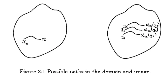
look at generalized baker's transformations with more slices. Let

fo

and

h

be measurable

functions on [0,1] such that

fo

+

h

=

1 almost everywhere and

Ii ~

C almost everywhere,

with respect to Lebesgue measure>. for i=O and 1. Then define

¢~(x)

=

l

x

fo(t)dt

¢~(x)

= ¢~(1)

+

foX

h(t)dt.

These maps are homeomorphisms of the interval onto their images, and the union of their

images is the whole interval. There is therefore a 2-branched expanding Lebesgue

measure-preserving map ¢, of which ¢o and ¢1 are the two inverse branches. Then the generalized

baker's transformation is defined as follows:

(

) _ { (¢(x),fo(¢(x))y)

Tf

x,y

-

(¢(x),l

- (fl(¢(x))(l

_y)))

if x

<

c, if x ~ c,

where c = ¢~(1). We will refer to this also as the generalized baker's tran.sformation based

on ¢, as the map ¢ is easily seen to determine the whole transformation, by noting that

¢'(x)

= 1/

fH¢(x))

almost everywhere, where iis 0 if

x

<

c and 1 if

x ~

c. Note that if we

consider the projection

p

sending points of S onto their first coordinate then

po'I']

= Tf

op,

so the pair (Tf, >. x >.) may be factored through this projection. The result of this is just the pair (¢,'>.). We call ¢ the vertical projection of T],

This situation is illustrated in Figures 2·1 and 2·2 below:

[image:40.547.109.399.48.665.2]

Figure 2·1 Possible graph of

<p.

Figure 2·2 Fundamental partition of Sunder TI'

The transformation operates as follows. The square is divided into two rectangles:

[image:40.547.147.395.54.318.2]