Original citation:
Ryan, M. S. and Nudd, G. R. (1993) Dynamic character recognition using hidden Markov models. University of Warwick. Department of Computer Science. (Department of
Computer Science Research Report). (Unpublished) CS-RR-244
Permanent WRAP url:
http://wrap.warwick.ac.uk/60927
Copyright and reuse:
The Warwick Research Archive Portal (WRAP) makes this work by researchers of the University of Warwick available open access under the following conditions. Copyright © and all moral rights to the version of the paper presented here belong to the individual author(s) and/or other copyright owners. To the extent reasonable and practicable the material made available in WRAP has been checked for eligibility before being made available.
Copies of full items can be used for personal research or study, educational, or not-for-profit purposes without prior permission or charge. Provided that the authors, title and full bibliographic details are credited, a hyperlink and/or URL is given for the original metadata page and the content is not changed in any way.
A note on versions:
The version presented in WRAP is the published version or, version of record, and may be cited as it appears here.For more information, please contact the WRAP Team at:
Dynamic Character Recognition Using
Hidden Markov Models.
1M. S. Ryan* and G. R. Nudd.
Department of Computer Science, University of Warwick, Coventry, CV4 7AL, England.
*e-mail address - ([email protected])
19th May 1993.
Abstract.
Hidden Markov Model theory is an extension of the Markov Model process. It has found uses in such areas as speech recognition, target tracking and word recognition. One area which has received little in the way of research interest, is the use of Hidden Markov Models in character recognition. In this paper the application of Hidden Mark-ov Model theory to dynamic character recognition is investigated. The basic Hidden Markov Model theory is reviewed, and so are the algorithms associated with it. A quick overview of the dynamic character recognition process is considered. Then three types of describing characters are considered, position, inclination angle of small vectors and stroke directional encoding using a Freeman code. A system using each of these de-scriptions, using Hidden Markov Models in the comparison stage, is described. It is rec-ognised that experiments using the different encoding systems have to be carried out to check the validity of this chosen method.
1. Introduction.
It is the purpose of this paper to investigate a form of pattern recognition known as character recognition, more specifically that of dynamic character recognition using Hidden Markov Models (HMMs) during the comparison stage of recognition. Dynamic character recognition uses information about the characters written by a person to iden-tify which characters have been written. The information generated by the handwriting process is captured by the computer at real-time, via the use of a digitising tablet, and is usually presented to the recognition system in the form of a time ordered sequence of x and y co-ordinates. This method of character recognition is also referred to as on-line character recognition, and has the advantage over static character recognition of not only containing static information such as position, but also dynamic information such as the order in which the character was written and dynamic features such as velocity and time taken to write the character.
as character recognition, which is the subject of this paper. Unlike the area of speech recognition, where HMMs have found extensive uses [1,2], there has been little work carried out on the use of HMMs in character recognition. Some work has been carried out in the area of static character recognition such as that carried out by Jeng et al [3], Tanaka et al [4], and Vlontzos and Kung [5], with very good results e.g. 91.5% to 97% recognition accuracy for multi-font Chinese characters in the case of Jeng et al, and 97% to 99% accuracy for the recognition of multi-font English characters in the case of Vlontzos and Kung for their two level character recognition system.
The area of dynamic character recognition using HMMs does not seem to have been considered in the literature. Nag et al [6] have carried out work in the area of dynamic cursive word recognition, using quantised inclination angles of small vectors to de-scribe the script making up the word. Cameillerapp et al [7] work concerns the recog-nition of on-line cursive handwriting using fully connected models of a full word, and stroke directions as features. The reason for choosing to model a word instead of indi-vidual characters is so that segmentation does not have to be carried out on the word, which is particularly difficult when the characters run into each other. But this leaves the problem of needing a separate model for each word to be recognised.
The motivation behind the use of HMMs in character recognition is the great variation of handwriting between different writers, and even in the same writer over a long time. Other reasons for the choosing of HMMs in the recognition of dynamic characters is that only the number of states, and the constraints to be imposed on the model have to be decided upon. Any rules about the nature of the characters can be established by ex-ample during the training phase of each HMM. HMMs also remove the need of explicit time alignment associated with the use of other techniques such as dynamic program-ming, or even Markov Models such as those used by Farag to model hand-written cur-sive words, [8].
In this paper, the concept of HMMs and various algorithms and implementation issues surrounding HMMs is examined in Section 2. Then a short description of the various processes involved in dynamic character recognition is considered in Section 3. In Sec-tion 4 the applicaSec-tion of HMM theory to dynamic character recogniSec-tion is considered, using three different types of character description.
2. Hidden Markov Models.
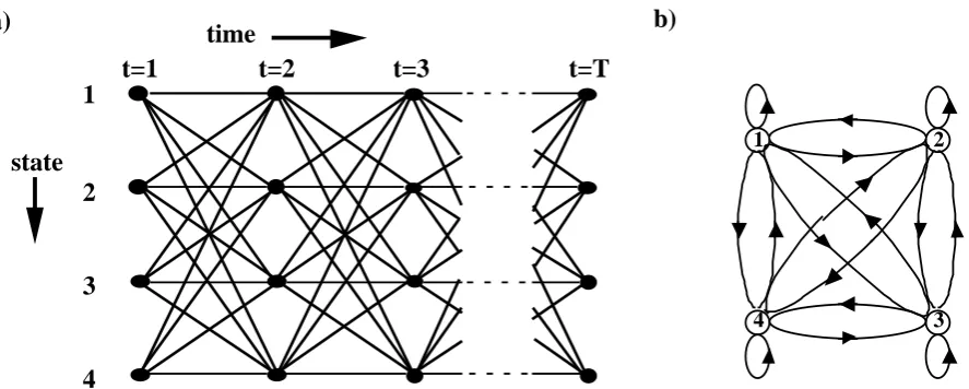
Figure 1. Showing a) Trellis Diagram and b) corresponding graph of 4 state HMM.
The actual structure of the Finite State Machine to be modelled by the HMM is hidden from view, therefore the structure of the HMM is usually a general one to take into ac-count all the possible occurrences of the states, with the HMM's states and transitions being estimates of the true underlying Finite State Machine. Associated with each tran-sition and observation symbol for a particular HMM are a set of metrics, which are used to obtain a measure of likelihood that the observations seen were produced by the mod-el represented by the HMM. Another type of Finite State Machine that is similar in na-ture to a HMM is a Markov Model. Markov Models have found extensive use in communications, [9], where the underlying process is known, i.e. all the possible states and transitions are known for the signal to be modelled. Only the observation process is statistical in nature, due to the noise introduced into the observation, though what ob-servation is produced by which state is also known. In this case only the Viterbi Algo-rithm, see section 2.2, is needed to decode the output.
Before looking at the various aspects of HMMs and the algorithms associated with them some notation associated with HMMs has to be defined as follows
:-t - The discre:-te :-time index.
N - Total number of states in the FSM.
M - Total number of possible observation symbols.
- The ith state of the FSM.
- The observation sequence generated by the process to be
modelled. Each is a symbol from the discrete set V of
possible observation symbols.
time
t=1 t=2 t=3 t=T
state 1
2
3
4
a) b)
1 2
4 3
xi
O= Ο1,Ο2,K ,OT
[image:4.595.77.521.82.260.2]- The set of the M different possible observation symbols,
usually an optimal set, where each symbol is discrete in nature. A single member of this set is represented by the symbol .
- The state sequence for the corresponding observation sequence.
- The survivor path which terminates at time t, in the ith state of the FSM.
It consists of an ordered list of 's visited by this path from time t = 1 to
time t.
T - overall length of the observation sequence.
- Initial state metric for the ith state at t = 0. Defined as the probability that
the ith state is the most likely starting start, i.e. .
- The transition metric for the transition from state at time t - 1 to the
state at time t. Defined as the probability that given that state occurs at
time t - 1, the state will occur at time t, i.e. ,
known as the Markovian property. These metrics can also change with time.
- The observation metric at time t, for state . Defined as the probability
V= ϖ{ 1,ϖ2,K , vM}
vk
I = ι1,ι2,K ,iT
spt( )i
xi
πι
Prob x( i at t = 0)
aij xi
xj xi
xj
Prob x( j at t xi at t -1)
bj( )k
that the observation symbol would occur at time t, given that we are in
the state at time t, i.e. . This metric is fixed for the
state regardless of where the state was entered.
- The survivor path metric of . This is defined as the Product of the
metrics (, and ) for each transition in the ith survivor path,
from time t = 0 to time t.
- compact notation used to represent the model itself, where A is
the 2 dimensional matrix of the 's, B is the 2 dimensional
matrix of the 's, andΠ is the 1 dimensional matrix of the
for the given model.
Before looking at the problems and algorithms associated with HMMs, it should be pointed out that the observation symbols considered throughout this paper are discrete. Though HMMs can be adapted to handle continuous symbols for the observations quite easily, by handling the probability densities as continuous. This adaptation is beyond
the scope of this paper, and has been investigated by other authors such as Rabiner in [1].
To allow a HMM to be used in real world applications, 3 problems have to be solved associated with the model process. These are
:-1. How to compute the likelihood of the observation sequence ,
given the model and observation sequence.
2. How to find the optimal underlying state sequence given the observations i.e. finding the structure of the model.
vk
xj
Prob v( k at t xj at t)
Γτ( )ι
spt( )i
πι
aij
bj( )k
λ = Α,Β, Π( )
aij
bj( )k
πι
bj( )k
3. How to train the model i.e. estimate A, B,Π to maximise .
Having established these as the problems that have to be dealt with in some manner, which look at some solutions to these three problems.
2.1 The Forward-Backward Procedure.
The solution to problem 1 above is based upon the forward-backward procedure. With the forward procedure the forward probabilities for the model are calculated. This prob-ability can be defined as the joint probprob-ability that the partial observation sequence and
a state at t of occurs given the modelλ, i.e. . This can be computed recursively by the
following algorithm
Initialisation
:-(1a)
Recursion
:-(1b)
Termination
(1c)
This can be used to score the model, but is also used during the re-estimation stage to obtain partial observation probabilities for states at each time interval.
There is also a need to define a backward procedure to calculate the backward prob-abilities for the model, but these are only used during the re-estimation stage, and is not
Pr ob O( λ)
O1,K ,Ot
( )
xi
ατ( ) = Προβ Οι ( 1L Ot,it = ξιλ)
α1( ) = πι ιβι( )Ο1 ∀ι ωηερε 1≤ ι ≤ Ν.
For t =1,2,K ,T -1 and∀ϕ ωηερε1 ≤ ϕ≤ Ν.
ατ+1( ) =ϕ ατ( )αι ιϕ
ι=1 Ν
∑
βϕ(Οτ+1)
Pr ob O( λ) = αΤ( )ι
ι=1 Ν
part of the solution to problem 1. A backward probability can be defined as, which is
the probability of the partial observation sequence from time t+1 to T, given the present state is at t, and given the model,λ. This can be calculated recursively by the following
algorithm
Initialisation
:-(2a)
Recursion
(2b)
So it can be seen that both the forward and backward probabilities are defined for all t, from 1 to T. The 's and 's produced by the above algorithms rapidly approach zero
numerically and this can cause arithmetic under flow, so a scaling technique is re-quired. A re-scaling technique is derived for 's in [1], and a similar re-scaling algorithm
can be defined for the 's. This technique requires all 's at a particular t to be re-scaled
if one of the 's falls below a minimum threshold, so that under flow is prevented. The
re-scaling algorithm for the 's at a particular t is given by equation 3
:-(3)
This re-scaling algorithm can be used at each iteration of the Backward procedure or only when one of the 's at a particular time is in danger of causing arithmetic under flow,
βτ( ) = Προβ Οι ( τ+1,Οτ+2,K ,OT it = ξι, λ)
xi
βΤ( ) = 1ι ∀ι ωηερε1 ≤ ι ≤ Ν.
βτ( ) =ι αιϕβϕ(Οτ+1)
ϕ=1 Ν
∑
βτ+1( ) ∀ι ωηερε1 ≤ ι ≤ Ν.ϕατ( )ι βτ( )ι
ατ( )ι
βτ( )ι ατ( )ι
ατ( )ι
βτ( )ι
ˆ
βτ( ) =ι βτ( )ι
βτ( )ι
ι=1 Ν
∑
a minimum threshold measure is used to judge when this is going to occur.
2.2 The Viterbi Algorithm.
The solution to problem 2 is based on the Viterbi Algorithm [10,11]. The Viterbi Al-gorithm finds the joint probability of the observation sequence and the specific state se-quence, I, occurring given the model,λ. most likely state sequence for the observation sequence given, , i.e. it finds the most likely state sequence. It is also usual to take the
natural logarithms of the A, B, andΠ parameters, so that arithmetic under flow is pre-vented in the Viterbi Algorithm during calculations. It should be noted that the Viterbi Algorithm is similar to the Forward Procedure in implementation, though the Forward Procedure sums over t and the Viterbi Algorithm uses a maximisation, and it also pro-vides the most likely state sequence. The algorithm can be calculated as follows
Initialisation
:-(4a)
(4b)
Recursion
(4c)
(4d)
where Append in equation (4c), takes the state and adds it to the head of the list of
the survivor path , whose transition had the maximum metric at t for the transition to Pr ob O, I( λ)
∀ι ωηερε1 ≤ ι ≤ Ν. Γ1( ) = λνπι ι + λνβϕ( )Ο1
sp1( ) = ξi [ ]ι
∀τ ωηερε2 ≤ τ ≤ Τ, ∀ϕ ωηερε1 ≤ ϕ≤ Ν. Γτ( ) = µαξϕ
1≤ ι≤ Ν[Γτ−1( ) + λναι ιϕ] + λνβϕ( )Οτ
spt( ) = Αππενδ ξj [ ϕ,σπτ−1( )ι ]
συχη τηατΓτ−1( ) + λναι ιϕ+ λνβϕ( ) = ΓΟτ τ( )ϕ
xj
state .
Decision
(4e)
(4f)
In English the Viterbi Algorithm looks at each state at time t, and for all the transitions that lead into that state, it decides which of them was the most likely to occur, i.e. the transition with the greatest metric. If two or more transitions are found to be maximum, i.e. their metrics are the same, then one of the transitions is chosen randomly as the most likely transition. This greatest metric is then assigned to the state's survivor path metric, . The Viterbi Algorithm then discards the other transitions into that state, and appends
this state to the survivor path of the state at t - 1, from where the transition originated. This then becomes the survivor path of the state being examined at time t. The same operation is carried out on all the states at time t, at which point the Viterbi Algorithm moves onto the states at t + 1 and carries out the same operations on the states there. When we reach time t = T (the truncation length), the Viterbi Algorithm determines the survivor paths as before and it also has to make a decision on which of these survivor paths is the most likely one. This is carried out by determining the survivor with the greatest metric, again if more than one survivor is the greatest, then the most likely path followed is chosen randomly. The Viterbi Algorithm then outputs this survivor path, ,
along with it's survivor metric, .
2.3 The Baum-Welch Re-estimation Algorithms.
The solution to problem 3 is based on a training method known as the Baum-Welch Re-estimation Algorithms, [12]. This algorithm finds a local optimal probability for ,
in this case a maximum. The re-estimation algorithms for the 3 model parameters,Π, A and B can be defined in English as follows, [1]
:-(5a)
xj
ΓΤ = µαξ
1≤ι≤ Ν[ΓΤ( )ι ]
spT = σπΤ(ι) συχη τηατΓΤ( ) = Γι Τ
Γτ( )ι
spT
ΓΤ
Prob O( λ)
(5b)
(5c)
where , and are the re-estimated parameters of the previous model parameters , and .
From the above definitions the following equations can be derived (see Appendix for the derivation of equations (6a), (6b) and (6c))
:-(6a)
(6b)
aij = εξπεχτεδ νυµβερ οφ τρανσιτιονσ φροµξι τοξϕ
εξπεχτεδ νυµβερ οφ τρανσιτιονσ φροµξι
bj( ) =k εξπεχτεδ νυµβερ οφ τιµεσ ινξϕ ανδ οβσερϖινγϖκ
εξπεχτεδ νυµβερ οφ τιµεσ ινξϕ
πι
aij
bj( )k
πι
aij bj( )k
πι = α1( )αι ιϕβϕ( )βΟ2 2( )ϕ
α1( )αν νµβµ( )βΟ2 2( )µ µ =1
Ν
∑
ν =1 Ν
∑
ϕ=1 Ν
∑
aij = ατ( )αι ιϕβϕ(Οτ+1)βτ+1( )ϕ
ατ( )αι ιϕβϕ(Οτ+1)βτ+1( )ϕ ϕ=1
Ν
∑
τ=1 Τ −1
(6c)
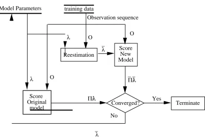
The notation represents the re-estimated model. The training of the model is carried
[image:12.595.97.499.392.664.2]out using a training set, consisting of observation sequences appropriate for that model. The training sequence can be summarised by the following diagram, Figure 2.
Figure 2. Showing training procedure for a HMM.
The scoring of the model depends on whether the Viterbi Algorithm or the Forward
bj( ) =k
ατ( )βϕ τ( )ϕ
ατ( )βι τ( )ι ι=1 Ν
∑
τ=1 σ.τ. οτ=ϖκΤ−1
∑
ατ( )βϕ τ( )ϕ
ατ( )βι τ( )ι
ι=1 Ν
∑
τ=1 Τ∑
λ = Α,Β, Π( )
Observation sequence
Score Original
model
Model Parameters training data
Procedure is to be used during recognition. If the Viterbi Algorithm is used then ,
whereas if the Forward procedure is used then . has the same meaning as P but
de-scribes the probability for the re-estimated model, . For each observation sequence in
the training set, the likelihood of the present modelλ, has to be compared with the new re-estimated model . If then the present modelλ is replaced by , meaning the new
mod-el is more likmod-ely to have produced the observation sequence than the previous modmod-el. The training procedure is then repeated on the same observation sequence, with , to see
if an even better model can be found. Convergence is reached when , or after a set
num-ber of re-estimation steps. Once convergence has been achieved for the present obser-vation sequence, then the new model is trained on the next obserobser-vation sequence in the training set, until there are no more observation sequences left in the training set. This training method is carried out on all the HMMs required for a system, using their own specific training data.
During each re-estimation stage, the Baum-Welch algorithms keep the statistical con-sistency needed when dealing with probability distributions i.e.
(7a)
(7b)
(7c)
The initial estimates of the probability densities for the model have to be established in some manner. According to Rabiner, [1], this can be achieved in a number of ways. A finite training set has to be used to train HMMs, usually due to the infinite variations that are encountered for a particular models. This means that special consideration has to be given to transitions or observation symbols that do not occur in the training set for
P= Προβ Ο,Ι λ( )
P= Προβ Ο λ( ) P
λ = Α,Β, Π( )
λ
P > Π
λ
λ = λ
P= Π
πι = 1
ι=1 Ν
∑
aij =1, φορ εαχηι ωηερε1 ≤ ι ≤ Ν.
ϕ=1 Ν
∑
bj( )k
κ=1 Μ
a particular model. This affects the 's and 's parameters, but the affect on the 's occurs
anyway due to the fact that only one will occur for each of the observation sequences
considered in the training set. If for example a particular observation does not occur in the training set then the value for that particular observation occurring will be set to
zero. It may be that this particular observation will never occur for that particular mod-el, but due to the finite nature of the training set there can be no assurance that it will not occur in the recognition stage. There are a few ways to deal with this problem ac-cording to Rabiner [1]. One is increasing the size of the training set, increasing the chance that all possible transitions and observation symbol occurrences associated with the model are covered. However this methods usually impractical both computationally and in obtaining the observation sequences for the training set. The model itself can be changed by reducing the number of states or number of observation symbols used, but the main disadvantage with this approach is that the model used has been chosen due to practical reasons.
Another method, and possibly the most appealing, is to add thresholds to the transition and observation metrics, so that an individual value cannot fall below a minimum value. This method is defined by Levinson et al in [13] for the 's, but it is redefined here for
clarity for the 's. If, for example, we set up a threshold for the 's as
(8)
then any for a particular i falls below this threshold then it is reset to the value . this is
done for all for a particular i. But, there is a need to re-scale the other 's which have not
fallen below so that the statistical consistency laid down by the condition given in
equation (7b), can be kept. To do this re-scaling the following equation has to be used
:-aij bj( )k
πι
πι
bj( )k
bj( )k
aij
aij
aij ≥ ε
aij
ε
aij aij
(9)
where is the minimum threshold set, is the re-scaled , l is the number of 's in the set ,
which in turn is the set of all the 's which fell below for a particular i. This process is
continued until all the 's for a particular i met the constraint. The re-scaling algorithm
for the 's is similar. This algorithm can be used after each step of the re-estimation
pro-cess, or after the whole re-estimation process for a particular observation sequence is completed.
It can now be seen that in most cases all three algorithms, i.e. the Forward-Backward Procedure, the Viterbi Algorithm and the Baum-Welch re-estimation Algorithms, are used during the training stage. Once training is complete, then the models can be used to recognise the objects that it represents. During recognition, the Viterbi Algorithm or the Forward Procedure are used to score the unknown observation sequence against the model/s to be considered. The forward Procedure can be dropped in favour of the Vit-erbi Algorithm, since in a majority of applications either the most likely state sequence has to be known, such as in target tracking [14] or word recognition [15], or the maxi-mum of is also the most significant term in , [16].
2.4 Types of HMM.
An important aspect of implementing HMM theory in real world applications, along with such matters as the number of states to use and the observation symbols to use, is the type of HMM to use. The two most commonly used types of HMMs, are the
˜
aij = 1 − λε( )
αιϕ
αιϕ,∀ϕ∉ ∀ϕα{ ιϕ< ε}
∑
, ∀ϕ∉ ∀ϕα{ ιϕ< ε}ε
˜ aij
aij aij
∀ϕαιϕ< ε
{ }
aij
ε
aij
bj( )k
Pr ob O, I( λ)
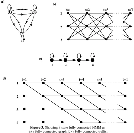
Figure 3. Showing 3 state fully connected HMM as a) a fully connected graph, b) a fully connected trellis,
and c) a left-to-right model for a 2-transition 4 state model and d) it's corresponding trellis diagram.
ergodic type models and the left-to-right models. The ergodic models are the type of model already considered in this paper, which are fully connected models, i.e. each state can be accessed at the next time interval from every other state in the model. An example of a 3 state ergodic model is shown in Figure 3.a in the form of a connected graph, and with the corresponding trellis diagram in Figure 3.b. The most important thing to note about the ergodic models are that the's are all positive.
The other main type of HMM, the left-to-right model is used to model signals that change properties over time, e.g. speech. This type of HMM has the unique property that a transition can only occur to a state with the same or higher state index i, as time increases, i.e. the state sequence proceeds from left to right. This means that the's have
a)
t=1 t=2 t=3 t=T
1
2
3 b)
1 2
3
c)
1 2 3 4
t=1 t=2 t=3
1
2
3
4
d) t=4 t=5 t=T
aij
the following property
(10)
and that the initial state is only entered if it begins in state 1,
(11)
it also means that the last state N has the following property
(12)
since the state sequence cannot go back along the model. An example of a 2 transition, 4 state left-to-right model is shown in Figure 3.c.
Even with these constraints placed on this type of model, the same algorithms are used without any modifications. So if a state becomes zero ant time during the training then it stays at zero from then on. The above two types of HMMs are the two most used HMMs, there are many variations on the theme, and the decision to use which model should be based on the application and the signals to be modelled.
For a more detailed analysis of the issues connected with HMMs discussed in this sec-tion and other issues, the reader is pointed to the work of Rabiner, [16] and [1].
3. Dynamic Character Recognition.
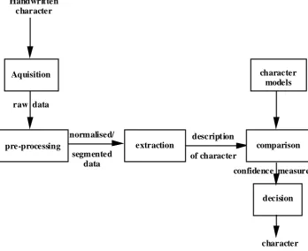
Before describing the system using HMMs in the next section, a brief look at the var-ious stages associated with dynamic character recognition is taken. Since character rec-ognition is a form of pattern recrec-ognition, it shares many of the same processes as other forms of recognition within this broad base of problems. These are show in Figure 4 below.
aij = 0, ιφϕ< ι.
πι =1, ιφι =1.0, ιφι ≠ 1.
aNN =1,
Figure 4. Showing processing stages of Character Recognition.
Acquisition in dynamic character recognition is usually carried out by a digitising tab-let. This supplies raw digital data in the form of and co-ordinate data of the pen
posi-tion on the paper. This usually comes with pen-down/pen-up informaposi-tion, a single bit, to indicate whether the pen is in contact with the paper or not. Some special pens have been developed to extract specific dynamic features such as force, [17], but have found better use in such areas as signature verification [18].
Pre-processing is the process where raw data is taken and various processing steps are carried out to make data acceptable to use in the extraction stage. This stage reduces the amount of information needed, removes some of the noisy data, and normalises it to certain criteria. Segmentation of the characters is the first process carried out, so that characters are presented to the comparison stage isolated from each other. The individ-ual character is then smoothed and filtered to remove noise from such sources as the digitiser, and human induced noise such as pauses during the writing process. It also removes redundant and useless information such as isolated points, which could cause misclassification. The final stage of pre-processing to be carried out on the character is that of normalisation. The character is normalised according to size, rotation and loca-tion depending upon the descriploca-tion of characters that is used for comparison. Some or all of these stages are carried out depending upon features used in the comparison stage. Once pre-processing has been carried out on the data, the next stage carried out on the data is a extraction stage. In this stage a meaningful description of the character to be recognised has to be extracted from the data provided by the pre-processing stage. It should be said that this part of the character recognition process is the most important, though what makes a good description of a character is not really known. Some typical
extraction Aquisition
pre-processing Handwritten
character
raw data
normalised/
segmented data
description
of character
decision comparison
character models
character confidence measure
x t( )
semi-circles are contained within the character, e.t.c. Others include transform co-effi-cients such as those generated by Fourier transforming characters. other descriptions can be based on dynamic characteristic such as positional order, direction of the writing to the horizontal or force exerted by the writer on the paper.
The last two stages are the comparison and decision stages, where the description of the unknown character is compared to models of the different known characters. The comparison stage can sometimes be split into two stages. The first stage, if implement-ed, reduces the number of possible character models that the unknown character has to be compared against. This is achieved by using such methods as dynamic programming or using such criteria as the presence of a dot or no dot. The next stage is the comparison of the unknown character description against some or all the models of known charac-ters. This stage can produce a confidence measure, based on a minimal, statistical or Euclidean distance measure, of how close the fit is between the unknown character and each of the character models in the systems. The decision stage then decides which model more closely resembles the unknown character and outputs the character with the best measure as the final decision. Decision trees can also be used during the com-parison-decision stage, particularly if shapes make up the description of the unknown character.
A more detailed analysis of the different stages and techniques used in dynamic char-acter recognition can be found in [19] and [20].
4. Use of HMMs in Character Recognition.
In this section a dynamic character recognition system using HMMs in the compari-son stage is investigated. For purposes of this first paper only the areas of extraction, comparison and decision will be considered initially, it will be assumed that a character has been acquired and pre-processed to the requirements of the system, though some normalisation and quantisation techniques are presented which are specific to a partic-ular descriptive method.
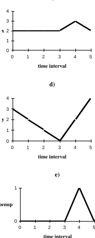
In this system, the character just written by a person is represented by a sequence of co-ordinates in the x and y directions, an example of a character 'i' that has been cap-tured dynamic by using a digitising tablet is shown in Figure 5.
a)
(x,y,penup)t = (2.0,3.0,0)0, (2.0,2.0,0)1, (2.0,1.0,0)2, (2.0,0.0,0)3, (3.0,2.0,1)4, (2.0,4.0,0)5.
0 1 2 3 4 0
1 2 3 4
Figure 5. Showing a) data sequence obtained from digitiser for character 'i', b) x-y plot of character 'i' for pendown positions only,
c) x-t plot, d) y-t plot and e) penup-t plot for the data sequence of the 'i'.
As can be seen in Figure 5, the character 'i' can be represented by four distinct vari-ables, notably the x, y, penup and the time interval data. The majority of English char-acters are written with one continuous stroke, as opposed to the two that are usually associated with characters such as 'i' and 'x'. It is initially proposed to look at the recog-nition of the 26 lower case letters of the English alphabet, but the system should be eas-ily adapted so that capital letters and digits can be recognised as well.
c)
time interval x
0 1 2 3 4
0 1 2 3 4 5
d)
time interval y
0 1 2 3 4
0 1 2 3 4 5
e)
time interval penup
0 1
4.1 And Position Description Method.
In this method the co-ordinates obtained from the digitiser are used as a description of each character. For each character to be used either in training or recognition, two observation sequences are generated for the HMM comparison stage. These two obser-vation sequences are which represents the normalised x co-ordinates observed up to
time , and which represents the corresponding normalised y co-ordinates for the same
time interval as that for , i.e. T in both observation sequences is the same. Each
obser-vation sequence contains points representing the position of the pen at that time, and also contains the character p to represent the penup code if the character contains more than one stroke, as in the case of a 't' or 'x'. Let the points that occur between penups be referred to as a segment. Note that the penup symbol will appear at the same time inter-val in both observation sequences. An example of the coding of the letter 'i' as shown in Figure 5 above, using this method
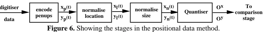
is:-Figure 6. Showing the stages in the positional data method.
Figure 6 shows the various stages involved in constructing the observation sequences for the comparison stage, for this method. The pre-processing stage for this method consists of three stages, the first being to find penups in the digitiser data, the second being the normalisation of the character's location, and the last stage is normalising the character for size. The first stage of encoding penups extracts the penup data at each point in the sequence obtained from the digitiser, and sets the and to the symbol 'p' at
a particular time interval, if the penup bit is set to 1, i.e. a penup has occurred at this
x t( )
y t( )
Ox = Ο( 1ξ,K ,OTx)
t = Τ Oy = Ο( 1ψ,K ,OTy)
Ox
Ox = (0.0,0.0,0.0,0.0, π,0.0).
Οψ= (0.8,0.6,0.2,0.0, π,1.0).
normalise location
normalise
size Quantiser
Ox
Oy
To comparison
stage xn(t)
yn(t) xl(t)
yl(t) encode
penups xp(t)
yp(t) digitiser
data
x t( )
[image:21.595.76.516.523.577.2]time interval, equation 13 where is the length in time of the digitiser data sequences
and .
(13)
This stage produces the and sequences to be used in the normalisation stage. The
character 'i' that has been considered as an example would have the following sequenc-es as output of the encode penups stage
The first stage of the normalisation process, normalising for location, finds the mini-mum and values over whole of the encoded penup sequences, and , this includes extra
segments for that character, e.g. a character x is made up of two segments and some penup values. It should be noted that penup values are ignored when finding the mini-mum value in either direction. To find the minimini-mum point in the x direction the follow-ing algorithm can be used, equation (14a).
Td
x t( )
y t( )
∀τ ωηερε1 ≤ τ ≤ Τδ, ιφ( πενυπτ≠ 0) τηεν
ξπ( ) = πτ ψπ( ) = πτ ενδιφ
xp( )t yp( )t
xp( ) = (2.0,2.0,2.0,2.0, π,2.0).t
ψπ( ) = (3.0,2.0,1.0,0.0, π, 4.0).τ
(14a)
(14b)
Once the minimum point has been found then the minimum value in the x direction, , is subtracted from all the values in the observation sequence, except for penup points,
using equation (14b). This process is also carried out on the values using found by
us-ing equation (14a) replacus-ing x by y, and then carryus-ing out the subtraction stage usus-ing equation (14b) as for the x values previous. This process produces two sequences of data and which are now passed onto the next normalisation stage. An example of the
encoded sequence produced by the normalise location process for the character 'i' in Figure 5 is
:-min _ x = ∞;
∀τ ωηερε1 ≤ τ ≤ Τδ, Ιφξπ( ) ≠ π τηεντ
Ιφξπ( ) < µιν _ ξ τηεντ µιν _ ξ = ξπ( )τ
∀τωηερε1 ≤ τ ≤ Τδ, Ιφξπ( ) ≠ π τηεντ
ξλ( ) = ξτ π( ) − µιν _ ξτ ελσε
ξλ( ) = ξτ π( )τ
min _ x
xp( )t
yp( )t
min _ y
xl( )t
yl( )t
xl( ) = (0.0,0.0,0.0,0.0, π,0.0).t
After normalising for location, each character is normalised for size by normalising each point in both location normalised sequences, and , to a value between 0 and 1.
This is done by finding the maximum value in each of the input sequences and then di-viding each point in by , and the same for the sequence. This size normalisation
pro-cess can be carried out for the data sequence by using the following equations, equation
(15a) to find and equation (15b) to calculate the normalised component .
(15a)
(15b)
This final stage of pre-processing produces two normalised data sequences, and , and
xl( )t yl( )t
xl( )t
max _ x
yl( )t
xl( )t
max _ x
xn( )t
max _ x = 0;
∀τ ωηερε1 ≤ τ ≤ Τδ Ιφξλ( ) ≠ π τηεντ
Ιφξλ( ) > µαξ_ ξ τηεντ µαξ _ ξ = ξλ( )τ
∀τωηερε1 ≤ τ ≤ Τδ,
Ιφ(ξλ( ) ≠ 0) ορ(ξτ λ( ) ≠ π) τηεντ
ξν( ) =τ ξλ( )τ
µαξ _ ξ ελσε
ξν( ) = ξτ λ( )τ
xn( )t
an example of these sequences for the character 'i' shown in Figure 5
After this stage a quantisation stage is carried out which quantises the normalised po-sition data, and , to a set of discrete evenly spaced points. This process also determines
the number of observation symbols to be considered by the HMM for each letter. To carry out the quantisation process on the data from the normalisation process, a gate size has to be determined for both the x and y data sequences. This value can be the same or different for both gate sizes, depending upon how many observation symbols the HMMs for the x and y data sequences of a character have.
Let the gate sizes of the x and y data sequence quantisers be and respectively. It will
be initially assumed that , and so the gate size for both the x and y data sequences can
be represented by . Only this gate size , or and , has to be specified for the quantiser,
all other factors associated with the quantiser can be calculated as follows from this gate size. From , the number of different possible quantisation levels, R, can be calculated
using equation (16).
(16)
where the addition of the 1 is needed to allow the inclusion of the 0.0 quantisation level. The set can be defined as the set of possible quantisation level values where is a
spe-cific quantisation level value and can be calculated by the following equation, equation (17).
xn( ) = (0.0, 0.0,0.0,0.0, π,0.0).t
ψν( ) = (0.75,0.5,0.25,0.0, π,1.0).τ
xn( )t yn( )t
gx
gy
gx = γψ
g g gx
gy
g
R= 1
γ + 1
Q
(17)
The and observation sequences can be constructed from the corresponding and data
sequences by the following quantisation equation, equation (18).
(18)
where and can be substituted with their y counterparts to obtain the quantisation
equa-tion for the y data sequence. These quantised values of the pendown and values, along
with the penup points make up the observation sequences, and , which will be used by
the HMMs in the comparison and decision stage to determine which character was writ-ten, see section 4.4. The number of observation symbols, M, generated by this method can be calculated from the following equation, equation (19), where the extra symbol p is generated by the encode penup stage.
(19)
If is considered for the gate size of the quantiser for the example character 'i', 6
quan-tisation levels are obtained for both the x and y quantisers. The resulting observation sequences obtained from this quantising stage will be
:-qr = γ × ρ−1( )
Ox Oy xn( )t yn( )t
∀τ ωηερε1 ≤ τ ≤ Τδ, ιφ ξ( ν( ) ≠ πτ ) τηεν
Οτξ= θ
ριφ θρ−
γ 2
≤ ξν( ) ≤ θτ ρ+
γ 2
ανδιφθρ∈Θ
ελσε Οτξ= ξ
ν( )τ
Ot x
xn( )t
xn( )t
yn( )t
Ox Oy
M= Ρ +1
This will also mean that there are 7 observation symbols for each model to be consid-ered in the comparison stage, i.e. the 6 quantisation levels of 0.0, 0.2, 0.4, 0.6, 0.8, and 1.0, and the symbol p for penup.
4.2 Inclination Angle of Vectors Description Method.
[image:27.595.102.498.411.458.2]This form of describing the character read in from the digitiser, is based on the ideas suggested by Nag et al, [6]. They describe a system for cursive word recognition, i.e. each HMM represents the whole word but each word is described as a sequence of quantised inclination angles, with special codes to represent sharp turning points. In our system using this descriptive method, the quantised inclination angles will make up the majority of the observation sequence for the comparison stage, but special codes for penups and single dots will also make up some of the set of possible observations. The special code used by Nag in his work, i.e. the sharp turning point code, will be imple-mented in our system later to see if better recognition results are obtained.
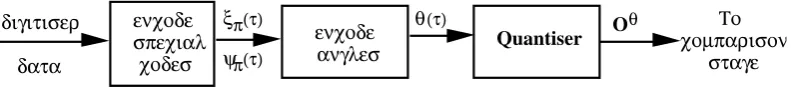
Figure 7. Showing the stages in the inclination angle method.
Figure 7 above, shows the various stages involved in constructing the observation se-quence for this method. It will become obvious to the reader that there are no normali-sation stages required in this method since the inclination angle of a small vector, that is used as the main observation feature, is size and location independent for any hand-written character.
The first stage of encoding the digitiser data for a character involves encoding penups into the and data sequences, as was done for the positional method, see section 4.2.
The other special code introduced at this encode special codes stage, is that for a dot, as is found in the characters 'i' and 'j'. This is needed particularly in the case of a char-acter i to distinguish it from an l. A dot can be defined as a point where a penup occurs at the previous and the next time interval in the digitiser data sequence. If the present point is the last in the digitiser data sequence and the previous one was a penup, then the present point can be classified as a dot. This will be the most commonly written form of a dot since in the majority of cases the dot in a character i or j is written last. To
Ox = (0.0,0.0,0.0,0.0, π,0.0).
Οψ= (0.8,0.6,0.2,0.0, π,1.0).
Quantiser Oθ χοµπαρισονΤο
σταγε ενχοδε
ανγλεσ θ(τ)
ενχοδε σπεχιαλ
χοδεσ
ξπ(τ) ψπ(τ) διγιτισερ
δατα
represent this special case a d is inserted at the point in the and data where the dot
oc-curred, by using the following algorithm, equation (20).
(20)
For the example character 'i' considered in the last section, the output from this encode special characters stage would be
The resulting sequences, and , are then feed into the next stage which encodes the
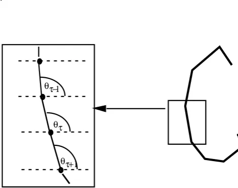
[image:28.595.176.411.512.697.2]inclination angles.
Figure 8. Showing Inclination angle for a sequence of small vectors of a letter c.
x t( ) y t( )
∀τ ωηερε1 ≤ τ ≤ Τδ,
ιφ πενυπ( τ−1≠ 0) ανδ τ = Τ(( δ) ορ πενυπ( τ+1 ≠ 0)) τηεν
ξπ( ) = δτ ψπ( ) = δτ ενδιφ
xp( ) = (2.0,2.0,2.0,2.0, π, δ).t
ψπ( ) = (3.0,2.0,1.0,0.0, π, δ).τ
xp( )t yp( )t
θτ θτ−1
In the next stage, encode angles, the and data sequences are encoded into one data
sequence - the sequence of inclination angles of consecutive points within each
seg-ment that makes up the character. Let represent an inclination angle of the vector
be-tween the points at t and at t+1, Figure 8. The inclination angle for each set of consecutive points can be found by the following equation.
(21)
where and are the changes in the x and y directions between consecutive points
respec-tively. So the output of this stage for the example character 'i' will be
:-where the angles are measured in degrees.
Once the angles have been worked out then they are passed onto the quantiser, as the data sequence. The quantiser stage quantises the angles in this data sequence to a set
number, , of possible angles. As for the quantiser in the previous method, section 4.1,
only the gate size of the quantiser in degrees has to be specified. only one quantiser is needed in this method and it's gate size can be represented by . The number of possible
angles, , can be calculated by adapting equation (16) as in equation (22).
(22)
Note that no additional 1 has to be added to equation (22) as in equation (16), this is because for this purpose, therefore no additional quantisation level has to be included
xp( )t
yp( )t
θ τ( )
θτ
θτ= ταν−1 ∆ψπ
∆ξπ
= ταν−1 ψπ(τ +1) − ψπ( )τ
ξπ(τ +1) − ξπ( )τ
∆ξπ ∆ψπ
θ τ( ) = (270,270,270, π,δ).
θ τ( )
Rθ
gθ
Rθ
Rθ =360
γθ
for . As for the quantiser in section 4.1, the set represents the set of possible
quantisa-tion level values and can be calculated as in equaquantisa-tion (17) in secquantisa-tion 4.1. The
observa-tion sequence which is passed onto the comparison stage can be constructed from the corresponding data sequences by using the same quantisation equation, equation (21),
as was used for the position method by substituting the values defined here into the equation. The number of observation symbols, M, generated by this encoding method can be found using equation (23).
(23)
Where the additional 2 symbols generated are the special codes for dots and penups. An example of the final observation sequence generated by this method for the example character 'i', where , thus giving the number of different possible observation symbols
of 74,
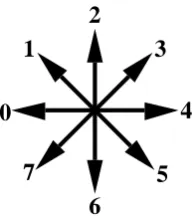
is:-4.3 Directional Encoding Method.
This method is based upon the work by Farag on cursive word recognition, [8]. Farag did not use HMM but Markov Models to represent each word that had to be recognised by the system, using time dependent transition matrices. This caused problems when there was not one-to-one correspondence between the word to be recognised and the model of the word, which would need to be solved by the use of dynamic programming to allow non-linear time warping of each word to fit it to the same time length as the model. In Farag's method each word was described by a direction code of each vector connecting consecutive points that make up a word. The directional encoding scheme only allowed 8 possible directions each vector could have, as is shown in Figure 9.
0°
Q= θ{ 1,K ,qr,K ,qR}
qr
Oθ
θ τ( )
M= Ρθ + 2
gθ = 5
Figure 9. Showing directional coding scheme.
The directional encoding scheme is sometimes referred to as a Freeman chain code in the literature, and it can be argued that this method is the same as Nag's inclination an-gle method. Figure 10 shows the various stages involved in constructing the observa-tion sequence, , for this method when adapted to dynamic character recogniobserva-tion.
Figure 10. Showing the stages in the directional encoding method.
The first stage of encoding the digitiser data is the same as the previous method, i.e. encoding the special codes for penups and dots, and the data sequences and will be the
same for both methods. The encode direction stage encodes the direction of writing for consecutive points at t and t+1 to one of eight possible directions. This can be done by using the equation given in [8], as reproduced here, equation (24).
(24)
where and are defined as for the previous method in section 4.2, and is the set of
pos-sible directions, in this case . Note that instead of the separate stages of calculating the
inclination angle and then quantising these angles, in this method these are carried out
0 1
2 3
4
5 6
7
Od
Od To
comp arison stage encod e
d irection encod e
special cod es
xp(t)
yp(t) digitiser
dat a
xp( )t
yp( )t
∆ψ ∆ξ = ι ιφ
πι 4 −
π 8
≤ ταν−1∆ψ∆ξ < πι4 + π8 ανδιφι ∈ φ
∆ξ ∆ψ
f
[image:31.595.152.444.357.404.2]in the same process. This process is carried out on all the pairs of consecutive points within a segment, for all segments in the and data sequences which are separated by
penups and do not include dots. The output of this process is the observation sequence which like the previous methods is passed onto the comparison stage. Using the
char-acter 'i' as the example, the observation sequence obtained by this coding method will be
This method generates 10 possible observation symbols, the 8 direction codes, and the penup and dot special codes. The major difference between this encoding method and the inclination angle encoding method presented in the previous section, is that the observation sequences passed onto the next stage in the inclination angle are in terms of degrees, whereas in the method considered in this section the output consists mainly of integers.
4.4 Comparison and Decision Processes.
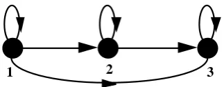
[image:32.595.215.377.606.669.2]Now that the encoding scheme to be investigated in our research, have been described in some detail, our attention is turned to the comparison and decision stages. Before de-scribing the actual comparison and decision processes, the HMMs to be used within the comparison stage have to be considered. For whatever encoding scheme used to con-struct the observation sequence/s the same general model can be used. The left-to-right HMM described in section 2.4 will be used to model each character to be recognised by the system. The first type of left-to-right model to be considered will be a 3 state model with skip states, Figure 11. This type of model will allow variations not just in the ob-servation data in a specific state, but it will variations in writing speed to occur, with the self-looping back into the same state taking into account slower than normal ing, and the skip state from state 1 to state 3 taking into account faster than normal writ-ing.
Figure 11. Showing a 3 state left-to-right HMM with skip states.
It should be noted that only one left-to-right model is required to represent each dif-ferent character in the inclination angle and directional encoding schemes, i.e. only 26 models are required to represent the 26 letters of the alphabet. In the poisitonal encod-ing method two left-to-right models are required for each character to be modelled in
xp( )t yp( )t
Od = Ο{ 1δ,Ο2δ,K ,OTd}
Od = (6,6,6, π,δ).
Though this number can be halved if the and are combined into one observation
se-quence as was done by Jeng et al [3].
Of course this type of model already constraints the and A matrices, which will
ini-tially be set as follows for all models in whatever description method used
:-where and A can be partially derived from the conditions laid down for left-to-right
models in section 2.4. What about the B matrix for each character? This will be differ-ent for each method, since the symbols are dependdiffer-ent on the way the observation se-quence is constructed. According to Rabiner, [1], only the B estimates have to be good estimates, but how are these estimates obtained. Rabiner suggest as number of methods including manual segmentation of observation sequences into states and then averaging observations within states, or maximum likelihood segmentation of observation se-quences with averaging within states or by the use of segmental k-means segmentation with clustering as considered by Rabiner in [1] and [21]. It is proposed for our system to use manual segmentation of a small number of observation sequences for each char-acter to be recognised, in the training set and using averaging within each state of the observations. For example, if the character i considered throughout this section as an example is used to build the observations, then using the observation sequence for the
example i as training data for segmenting and establishing the initial B matrix, the B matrix for the x HMM will be
:-where the rows represent the present state j, and the columns represent the possible ob-servation symbols, the 6 quantisation levels 0.0 to 1.0, and the last column represents the symbol p for penup. Note that the penup that occurs in the character i allows for easy segmentation of the observations between the states in the model.
Once the initial estimates for the B matrix for a particular character model have been established, then the training procedure begins. In this training period a number of
ob-Ox Oy
Π
Π = 1 0 0[ ]
A=
0.34 0.33 0.33 0.0 0.5 0.5 0.0 0.0 1.0
Π
Ox
B=
0.9994 0.0001 0.0001 0.0001 0.0001 0.0001 0.9994 0.0001 0.0001
0.0001 0.0001 0.0001 0.0001 0.0001 0.0001 0.0001 0.0001 0.0001
0.0001 0.9994 0.0001
servation sequences of the character the model is being trained to represent are used. The training procedure using the Baum-Welch re-estimation algorithms will be used to train each model, see section 2.3, but only the re-estimation algorithms for the and
have to be used, equations (6b) and (6c), since the constraint that the left-to-right model always starts in state 1 has already been set. The forward procedure described in section 2.1, will be used to score the models during training and recognition. The use of the Vit-erbi Algorithm, described in section 2.2, in scoring the models will also be investigated. For this system the character description just supplied to the comparison stage is com-pared to all the models formed during the training stage. The forward procedure is then used to compare the observation received from the extraction stage, to determine how likely the character read in matches each model in the system. This will produce a con-fidence measure for each model for that particular observation sequence, , where is the
cth character model. The more closely the observation sequence matches a particular model, the higher the confidence measure and the more likely that the character the model represents the unknown character just written. Once a confidence measure has been obtained for each model a decision can be made on which character model best represents the unknown character just written. The simplest criteria to use for this de-cision is to say that the character model which has produced the best confidence mea-sure is the unknown character. This decision stage can be represented by equation (25).
(25)
where is the total number of separate characters that are modelled in the system, in our
system and is the probability measure obtained by the forward procedure, for the
ob-aij bj( )k
Pr ob O( λχ) λχ
max _ prob= −∞
βεστ_ µοδ ελ= 1
∀χ ωηερε1 ≤ χ≤ Χ,
ιφ Προβ Ολ( ( χ) > µαξ_ προβ) τηεν µαξ _ προβ= Προβ Ο λ( χ) βεστ_ µοδ ελ = χ
ενδιφ
C
C= 26
servation sequence given the model, , for the cth character. The output of this stage is
the reference number for the best fitting model, c, and it's confidence measure, . In the
case of the position encoding method is given by combining the confidence measure
for the x and y HMMs, as is shown in equation (26).
(26)
Both equations (25) and (26) can be easily adapted if the Viterbi Algorithm is used to score the models instead of the forward procedure.
This would be the simplest form of character recognition, but no method of character recognition is perfect, so this is where higher level models can be used to correct wrong-ly recognised characters. Here we can see the inherent advantage of using HMMs in character recognition, since a confidence measure is produced for each character mod-el, not only can the most likely character be passed to higher level models, but the next n most likely characters along with their confidence measures can be passed, thus sup-plying higher level models with more information about the characters it has recogn-ised. This will be of more use when two character models have similar confidence measures. Such higher level models take into account the whole word, and then the sen-tence that each word is contained in. Such a system has already been developed for stat-ic character recognition by Vlontzos and Kung, [5], using Hidden Markov Models at the character and word levels. All that would have to be done to their system is substi-tute the static character system with one of the systems described in this section.
5. Summary and Conclusions.
The application of Hidden Markov Models to dynamic character recognition has been considered. A review of the theory and some of the implementation issues has been pre-sented. It should be noted that experiments need to be conducted to see how well the various methods suggested in this report are in reality. It should be obvious to the reader the advantage of the inclination angle and directional encoding schemes in that they re-quire no normalisation of the incoming data to derive a description.
An investigation into what type of model, left-to-right, ergodic or a mixture, best rep-resents the underlying Markov process in dynamic character recognition has to be car-ried, similar to the one suggested by Nag et al [6] for dynamic cursive word recognition. Also an investigation into what other types of descriptions can be used and how well they perform against the other method already described in this paper, especially what combinations of descriptions work best and which descriptions have little or no relevant information to the character.
Two obvious applications where the work presented in this paper can be used, are dy-namic signature verification and single writer adaptation. The dydy-namic signature veri-fication work would require adaptation of the methods presented in this paper, including the need of only on HMM to represent the signature, and the finding of more writer dependent features. The application of HMMs to dynamic signature verification
λχ
Prob O( λχ)
Pr ob O( λχ)
has been considered by Hanan et al in [22], representing the and position sequences
as a set of up and down slopes and the time interval for each of these slopes.
Another problem that is not considered in the literature is that of punctuation recog-nition, i.e. recognising such characters as ?, or ", though the recognition of mathemati-cal equations and line drawings have been considered, [23,24]. Whether it is static or dynamic recognition, this problem has to be considered just as important as the charac-ter recognition problem, and should really be considered as part of the same process. The reasoning behind this is that the English language is not just made up of letters which make up words, but digits and punctuation which give the language extra mean-ing, and allow us the distinguish between the end of one sentence and the beginning of another for example. If character recognition systems, both static and dynamic, are to become viable and accepted commercially for use in large scale document reading, then the ability to recognise punctuation has to be included.
Acknowledgements.
The authors would like to thank the members of the Parallel Systems Group in the Computer Science Department of the University of Warwick for their encouragement, help and useful discussions about character recognition and Hidden Markov Models.
Appendix. Derivation of Re-estimation Formulas for Model
Param-eters.
In this appendix the re-estimation formulas for , and are derived using the formulas
given in [1]. Before the derivation of the re-estimation formulas can be carried out, two more variables have to be introduced. The first is the state probability, , which can be
defined as the probability of being in state at time t, given the observation sequence
and the model, equation (A1).
(A1)
Equation (A1) can be expressed in terms of the forward-backward variables as in equa-tion (A2).
x t( ) y t( )
πι
aij bj( )k
γτ( )ι
xi
(A2)
To be able to derive the equations for and the probability of a particular transition
occurring has to defined. The branch probability, , can be defined
according to [1] as the joint probability that given the observation sequence and the model, that at time t the model is in state and at time t+1 the model is in state , equation
(A3). This can be expressed in terms of the model parameters, and the forward-back-ward variables as in equation (A4).
(A3)
(A4)
So the state probability , can be expressed in terms of the branch probability , as
shown in equation (A5).
(A5)
The derivation of the re-estimation formula for can now be looked at. From section
2.3, it can be seen that the definition of the re-estimation formula, equation (5a), for a γτ( ) =ι ατ( )βι τ( )ι
Προβ Ο λ( ) =
ατ( )βι τ( )ι ατ( )βι τ( )ι
ι=1 Ν
∑
πι
aij
ξτ( )ι, ϕ
xi
xj
ξτ( ) = Προβ ιι, ϕ (τ= ξι,ιτ+1= ξϕΟ,λ)
ξτ( ) =ι, ϕ ατ( )αι ιϕβϕ(Οτ+1)βτ+1( )ϕ
ατ( )αν νµβµ(Οτ+1)βτ+1( )µ µ =1
Ν
∑
ν=1 Ν
∑
γτ( )ι ξτ( )ι, ϕ
γτ( ) =ι ξτ
ϕ=1 Ν
∑
( )ι, ϕparticular initial state is the expected number of times in that state at . This can be
ex-pressed in terms of the state probability as in equation (A6).
(A6)
Looking at the right hand side of equation (A6) it can be seen that can be expressed in
terms of as in equation (A7). on the right hand side of this equation can be substituted
by the right hand side of equation (A4), as in equation (A8).
(A7)
(A8)
Substituting equation (A8) into (A6) and we obtain the following equation in terms of the model parameters and the forward-backward variables, equation (A9), for the re-estimation formula for .
(A9)
xi
t = 1
γτ( )ι
πι = γ1( )ι
γτ( )ι
ξτ( )ι, ϕ ξ1( )ι, ϕ
γ1( ) =ι ξ1( )ι, ϕ
ϕ=1 Ν
∑
ξ1( )ι, ϕ
ϕ=1 Ν
∑
= α1( )αι ιϕβϕ( )βΟ2 2( )ϕα1( )αν νµβµ( )βΟ2 2( )µ µ =1 Ν
∑
ν=1 Ν∑
ϕ=1 Ν∑
πιπι = α1( )αι ιϕβϕ( )βΟ2 2( )ϕ