A conservative finite difference scheme for Poisson–Nernst–Planck equations

DOI 10.1007/s10825-013-0506-3

A conservative finite difference scheme for Poisson–Nernst–Planck

equations

Allen Flavell·Michael Machen·Bob Eisenberg· Julienne Kabre·Chun Liu·Xiaofan Li

Published online: 25 September 2013

© Springer Science+Business Media New York 2013

Abstract A macroscopic model to describe the dynamics of ion transport in ion channels is the Poisson–Nernst– Planck (PNP) equations. In this paper, we develop a finite-difference method for solving PNP equations, second-order accurate in both space and time. We use the physical param-eters specifically suited toward the modeling of ion chan-nels. We present a simple iterative scheme to solve the sys-tem of nonlinear equations resulting from discretizing the equations implicitly in time, which is demonstrated to con-verge in a few iterations. We place emphasis on ensuring numerical methods to have the same physical properties that the PNP equations themselves also possess, namely conser-vation of total ions, correct rates of energy dissipation, and positivity of the ion concentrations. We describe in detail an approach to derive a finite-difference method that preserves the total concentration of ions exactly in time. In addition, we find a set of sufficient conditions on the step sizes of the numerical method that assure positivity of the ion

concen-A. Flavell·M. Machen·J. Kabre·X. Li (

_B

Present address: M. Machen

Department of Applied and Computational Mathematics and Statistics, University of Notre Dame, 153 Hurley Hall, Notre Dame, IN 46556, USA

B. Eisenberg

Department of Molecular Biophysics and Physiology, Rush Medical Center, 1653 West Congress Parkway, Chicago, IL 60612, USA

C. Liu

Department of Mathematics, Pennsylvania State University, University Park, PA 16802, USA

trations. Further, we illustrate that, using realistic values of the physical parameters, the conservation property is criti-cal in obtaining correct numericriti-cal solutions over long time scales.

Keywords Electrodiffusion·Finite difference·Ion channel modeling·Poisson–Nernst–Planck equations

1 Introduction

The Poisson–Nernst–Planck (PNP) equations describe the diffusion of ions under the effect of an electric field that is itself caused by those same ions. The system is created by coupling the Nernst–Planck equation (which describes the diffusion of ions under the effect of an electric poten-tial) with the Poisson equation (which relates charge den-sity with electric potential). This system of equations has found much use in the modeling of semiconductors [24]. Al-though the Poisson–Nernst–Planck equations were applied to model membrane transport for longer than they have been employed to model semiconductors [30], the use of the sys-tem to model the behavior of the internal mechanics of these transport processes is much more recent [8].

The system of PNP equations and its related models have been the subject of much study and numerical simulation. A recent advancement in this field was the application of energy variational analysis and density functional theory to modify the PNP system to accommodate various phenom-ena exhibited by biological ion channels. See [32] and the references therein.

two dimensions using a second-order accurate finite differ-ence method with central differencing in space and Crank– Nicolson scheme in time, and simulated an ion channel subjected to time-dependent perturbations. Nanninga (2008) [27] studied a nerve impulse using a similar finite difference scheme as in [3] but in three dimensions, notable in that it di-rectly included gating and selectivity into the model. Lopre-ore et al. (2008) [23] developed a finite-volume-based tech-nique to solve PNP in three dimensions, which decomposes the domain using a dual Delaunay–Voronoi mesh. Neuen (2010) [28] developed a semi-implicit finite element-based scheme to simulate three-dimensional, multi-scale extended PNP. Gardner and Jones (2011) [10] simulated a potassium channel modelled with PNP in two dimensions using a finite difference method with TR-BDF2 time integration. Much of the numerical schemes in [10] is based on the previous work [11], a one-dimensional model of the same channel. Hyon

et al. (2011) [19] presented another finite element method with back-Euler method in time to investigate the effects of finite size of the ions by modifying the PNP via introduc-ing a repulsive potential energy into the total energy. Horng

et al. (2012) [17] applied the multiblock Chebyshev pseu-dospectral method and the method of lines to solve a one-dimensional modified PNP modeling the finite-sizeness of the ions via a local model.

One of the characteristics of the nonlinear PNP equations is that its overall behavior is very sensitive to the boundary conditions [13]. This presents a challenge for accurate and efficient numerical simulations, as generally the boundary conditions will have to be discretized and approximated. In this paper, we shall investigate the effects of discretization error on the Poisson–Nernst–Planck equations, in particular discretization of the boundary conditions and the equations at the boundaries. We will demonstrate that the conserva-tion properties of the numerical methods could be critical in obtaining the long-time behavior of the solutions.

To our knowledge, relatively few studies describe numer-ical methods such as finite difference method, finite element method, finite volume method and many others for solv-ing partial differential equations (PDEs), which preserve

the physical quantities underlying the PDEs exactly at the discrete level. Fisher et al. (2012) [9] developed finite dif-ference methods for solving the Euler equations and the Burgers equation that relied on using specific split forms of the equations to preserve the discrete energy dynamics. Hof and Veldman (2012) [16] developed finite volume dis-cretizations for the 1D and 2D Euler equations, as well as the 1D and 2D Shallow Water equations, which conserved the dynamics of mass, momentum and energy of the sys-tems. For the incompressible Navier–Stokes equations, the papers [14,15, 20,25, 26,31] presented finite difference discretizations on uniform or nonuniform grids that preserve part or all of discrete mass, momentum, and kinetic energy.

Li and Vu-Quoc (1995) [22] developed a finite difference method for solving the nonlinear Klein–Gordon equation which preserved the total discrete energy. Qiao et al. (2011) [29] showed unconditionally energy stable finite difference schemes for the dynamics of the molecular beam epitaxy, which preserves the energy decay rate exactly at the discrete level. Zhang and Qiao (2012) [33] proposed a finite differ-ence scheme that is mass-conservative and preserves energy decay rate precisely for the Cahn–Hilliard equation. Celle-doni et al. (2012) [4] developed a general method of dis-cretizing partial differential equations that preserved the to-tal energy exactly, based on the average vector field method. Chiu et al. (2012) [5] developed a general meshfree scheme for solving partial differential equations characterized by conservation of the discrete energy, and they demonstrated its effectiveness by solving the 1D and 2D inviscid advec-tion equaadvec-tions.

It is also rare for numerical schemes to preserve posi-tivity for nonlinear advection-diffusion equations like PNP, which do not have a maximum principle. The work on this topic is well summarized by Hundsdorfer and Verwer[18]. Bolley and Crouzeix [2] developed much of the theory, es-tablishing that linear single-step and multi-step methods of second-order or higher in time cannot preserve positivity un-conditionally, and obtaining necessary and sufficient condi-tions for positivity preservation for certain classes of numer-ical methods.

The paper is organized as follows. We start by defin-ing and simplifydefin-ing the equations we are workdefin-ing with, in Sect.2, including the introduction of the quantities that shall be preserved by our numerical schemes: the total concen-tration of each ion species in Sect.2.1and the energy dis-sipation law in Sect.2.2. We then describe our numerical schemes in Sect.3, which presents an approach to conserve the total ion concentrations exactly, preserve positivity of the ion concentrations, and approximate the energy dissipation law closely. Finally, we shall discuss the results of simulat-ing the system ussimulat-ing our numerical schemes in Sect.4.

2 Governing equations

Consider the PNP equations [8,11]

∂ci

∂t =∇·

Di

∇ci+

zie

kBT

ci∇φ

, (1)

i=1,2, . . . , N,

∇·(∇φ)= −

ρ0+

N

i=1 zieci

, (2)

whereci is the ion density for the i-th species, Di is the

kBis the Boltzmann constant,T is the absolute temperature,

is the permittivity,φis the electrostatic potential,ρ0is the permanent (fixed) charge density of the system, and N is the number of ion species [19]. The equations are valid in a bounded domainΩ with boundary∂Ω and for timet≥0.

In this work, we shall use the no-flux boundary condition for Eq. (1). This may correspond to modeling the interior conditions of a channel that is in an occluded state, with closed gates at either end. Simulations of channels such as the KirBac1.1 channel in such a state have been conducted in the past [6]. We shall use the Robin boundary condition for the Poisson equation, which models the effects of mak-ing the source of the potential across the channel partially removed from the ends of the channel. The formula for the boundary conditions are

Di

∇ci+

zie

kBT∇

ciφ

·n=0, i=1,2, . . . , N, (3a)

(φ−φ_±)+η∂φ

∂n =0, (3b)

for points on the boundaryx∈∂Ω.

For some situations, such as a generic potassium chan-nel separating potassium and chloride ion baths, the experi-mental data can be well-approximated by a one-dimensional model [11]. In one dimension, Eqs. (1) and (2) are simplified as ∂ci ∂t = ∂ ∂x Di ∂ci ∂x + zie

kBT

ci ∂φ ∂x (4) ∂ ∂x ∂φ ∂x

= − ρ0+

i

zieci

, (5)

for−L≤x≤Landt≥0, whereLis the half of the length of the ion channel. The corresponding boundary conditions are

Di

∂ci

∂x + zie

kBT

ci

∂φ ∂x

=0,

(φ−φ_±)±η∂φ

∂x =0, forx= −L, L.

(6)

2.1 Total concentration

The total concentration per ion species is given by

ci,t ot(t )=

L

−L

ci(x, t )dx, i=1,2, . . . , N. (7)

Due to the no-flux boundary conditions (6), the total con-centration of each ion species is constant in time. This can be verified easily by differentiating (7) with respect to time, then applying the convection-diffusion equation (4) and no flux boundary condition (6).

One of the metrics we can use to evaluate different nu-merical schemes is therefore to measure how well the total concentration is conserved in numerical simulation. Ensur-ing that the total concentration for each speciesci,t ot is

con-stant will be the idea behind the schemes presented in this work. As will be seen in Sect.4, the preservation of the con-servation property is crucial for producing correct numerical results over long time scales.

2.2 Energy dissipation

The governing equations (4) and (5) for the transport of ions can be derived from the energy of the system using vari-ational principles. Similar to [19], the total energy for our specific system is defined by

E=

L

−L

kBT

N

i=1 cilog

ci

ci,0

+1 2

ρ0+

N

i=1 zieci

φ dx + 2η

φ₊φ (L)+φ₋φ (−L), (8)

whereci,0are constants called “reference concentrations”. Using the Poisson equation (5), the total energy can be writ-ten as

E=

L

−L

kBT

N

i=1 cilog

ci

ci,0+ 2 ∂φ ∂x 2 dx + 2η

φ2(L)+φ2(−L), (9)

where the last term is the contribution of the electric energy from the boundaries. The total energyEsatisfies the energy dissipation property

dE dt = −

L

−L N

i=1 Di

kBT

ci

∂μi

∂x

2dx, (10)

whereμiis the chemical potential ofi’th ion species defined

by the variational derivative of the energy with respect to the concentrationci

μi=

δE δci =

kBT log

ci

ci,0+ 1

+zieφ. (11)

The energy dissipation law (10) can be derived by taking the time derivative of the total energy (8) and applying integra-tion by parts, Eqs. (4)–(5) and the boundary condition (6):

dE dt =

L

−L

kBT

i

log ci ci,0+

1 ∂ci ∂t dx + L −L 1 2 i

zie

∂ci

∂t φ+ 1 2 ρ0+

i

zieci

∂φ

∂t

+ ∂ ∂t

2η

φ₊φ (L)+φ₋φ (−L)

= − L

−L

i

Di

kBT

ci

∂μi

∂x 2dx

−1 2

∂φ ∂x

∂φ ∂t −

∂2φ ∂x∂tφ

L

−L

+ ∂ ∂t

2η

φ₊φ (L)+φ₋φ (−L). (12)

The rate of energy decay (10) can be obtained by using the boundary condition (6) to show the last two terms on the RHS of (12) cancel each other.

2.3 Parameters and nondimensionalization

We specify the units and the parameters using the approx-imate values corresponding to the KcsA potassium chan-nel [7]. In our 1D model, the cylindrical channel takes a diameter of 10 Å and a length of 120 Å. We shall as-sume no permanent charges or selectivity for the purposes of this simulation. We consider the case of two ion species, i.e. N =2, with the initial concentration for each ion be-ing 2 molar, resultbe-ing in an initial number density (num-ber of ions per unit volume) of 1.2044×10−3 ions/Å3. The combination of the parameterskBT /eis approximately

0.025 V, assuming the temperature isT =298 K. The per-mittivity=r0is determined by the value of the vacuum 0=8.854187817×10−12 F/m and the relative permittiv-ityr (78.5 for water).

The values of the diffusion coefficients Di depend on

both the ion species and the channel. The only net effect of different diffusion constants is the rate of evolution of the system. Typical values for the diffusion coefficients for ion species in a channel are around 109Å2/s [12]. We will select both diffusion coefficients to be equal to each other, causing them to take a value of one after nondimensionalization.

The parameter η, as a component of the Robin bound-ary condition (3b), is an aggregate of multiple physical con-stants and is highly dependent on the properties of the sur-rounding membrane. modeling the experimental setup as an electrical circuit shows that the quantityAl/η, whereAis

the area of the membrane and l is the permittivity of the

membrane, has units of capacitance and is related to charge storage. The most significant charge storage contributing to Al/ηis in fact the membrane capacitance, so we may

sur-mise that the primary contributor toηis the membrane ca-pacitance. If a very high capacitance to ground is present, η is approximated by the appealing formula η=Al/C,

whereC is the capacitance of the membrane, however re-alisticallyηis much smaller than that. In this work, we shall takeη=2.78×10−3Å for our numerical simulations, but

will also examine the effects ofηover a range from 10−5Å to 60 Å. Changing the value ofηmight correspond to adding a parallel capacitance in experiment.

Define the dimensionless variables and parametersc_i= ci/c0,x=x/L,t=t /(L2/D0),D_i=Di/D0,φ=φ/φ0, and ρ₀ =ρ0/(ec0) where c0 is the average of the initial charge concentration, L is the half of the channel length or computational domain,D0 is a typical diffusion coeffi-cient,φ0is a characteristic value of the electrostatic poten-tial such as the boundary value. Then, non-dimensionalizing the Nernst–Planck equation (4), we obtain

∂c_i ∂t =

∂ ∂x

D_i

∂c_i

∂x +χ1 zic

i

∂φ ∂x

, (13)

whereχ1:=eφ0/ kBT. From the above, the dimensionless

parameterχ1≈3.1, ifφ0=0.08 V. The nondimensional-ized Poisson equation (5) is given by

∂

∂x

∂φ ∂x

= −χ2 ρ0+

i

zici

, (14)

whereχ2:=ec0L

2

φ0t . Here, the dimensionless parameter _is

defined as:=/t wheret is the characteristic

permit-tivity chosen to be the value for water:t=6.950537436×

10−20 F/Å. The non-dimensional parameterχ2is approxi-mately 125.4 with these values. The corresponding dimen-sionless boundary conditions are

D_i

∂c_i

∂x +χ1 zic

i

∂φ

∂x

=0,

φ−φ_± +η∂φ

∂n =0, forx= −1,1,

(15)

whereη:=η/L.

We drop the primes when we present our numerical meth-ods for clarity.

3 Numerical methods

method for solving the large nonlinear systems at each time step, we present a simple iterative scheme which is easy to implement and can solve the systems efficiently.

3.1 Discretization in time

For time-stepping, we shall use a slight modification of the scheme described in [1], which combines the trape-zoidal rule with the second-order backward differentiation formula.

(1) TR step:

cn_i+γ ,k+1−γtn 2 f

cn_i+γ ,k+1, φn+γ ,k

=cn_i +γtn 2 f

cn_i, φn, i=1,2,

∂

∂x

∂φn+γ ,k+1 ∂x

= −χ2

ρ0+

2

i=1

zicn_i+γ ,k+1

,

(16)

fork=0,1,2, . . .. (2) BDF2 step:

cn_i+1,l+1−1−γ 2−γtnf

cn_i+1,l+1, φn+1,l

= 1

γ (2−γ )c

n+γ i −

(1−γ )2 γ (2−γ )c

n

i, i=1,2,

∂

∂x

∂φn+1,l+1 ∂x

= −χ2

ρ0+

2

i=1

zicni+1,l+1

,

(17)

for l=0,1,2, . . ., where f (ci, φ)is defined as the

right-hand side of (13)

f (ci, φ)=

∂ ∂x

Di

∂ci

∂x +χ1 zici ∂φ ∂x

. (18)

We takeγ=2−√2, which minimizes the local truncation error [11].

Removing the inner iterations, corresponding to the in-diceskin (16) andl in (17), Eqs. (16) and (17) is the TR-BDF2 scheme requiring a nonlinear solver for the two sys-tems of nonlinear equations: (16) for (cn+γ, φn+γ) at the grid points and (17) for(cn+1, φn+1). With the inner itera-tions, Eqs. (16) and (17) provide a simple iterative scheme for solving the systems of nonlinear equations. For instance, at k-th iteration, we update the array cn+γ ,k+1 at the grid points by solving the first equation of (16) which is a tri-diagonal system after the spatial discretization, since the val-ues ofφn+γ ,k are known atk-th iteration; then, we update φn+γ ,k+1 using the second equation of (16). We perform the inner iterations until convergence and, as shown later, choosing two inner iterationsk=2 andl=2 would be suf-ficient. As for initial guesses at then-th time step, we choose

φn+γ ,0=φnfor (16) andφn+1,0=φn+γ ,k+1for (17) withk corresponding to the last inner iteration at the previous inner iteration. As shall be seen in Sect.4, without any such inner iterations (k=l=0), one could only attain first-order accu-racy in time; on the other hand, with just one inner iteration (k=l=1), one can attain second-order accuracy in time. In other words, the simple iterative scheme is very effective in solving the systems of nonlinear equations.

3.2 Discretization in space

Next, we provide the discrete equations for the spatial dif-ferential operators in Eqs. (16) and (17). Let’s divide the dimensionless interval[−1,1]toJsubintervals,xj= −1+

j x, wherex=2/J andj =0,1,· · ·, J. We denote the numerical values ofg(x, t )at(xj, tn)byg_jnandg(x)atxj

bygj. We present the standard second-order central

differ-encing schemes for the spatial differential operators here to facilitate the description of the mass-conservative scheme which depends on the details of the discretization at the in-terior grid points (1≤j≤J−1).

The ion diffusion term in Eq. (13) is discretized as

∂ ∂x Di

∂ci

∂x

(xj)

≈Di,j+12cj+1−(Di,j+ 1

2 +Di,j− 1

2)ci,j+Di,j− 1 2ci,j−1

(x)2 .

(19)

The term driven by the electrostatic potential gradient in Eq. (13) is given by

∂ ∂x Dici

∂φ ∂x

(xj)

≈Di,j+1ci,j+1(φj+2−φj)−Di,j−1ci,j−1(φj−φi,j−2)

4(x)2 .

(20)

The Laplacian in the Poisson equation (14) is approximated by

∂

∂x

∂φ ∂x

(xj)

≈ 1 (x)2

_j+1

2φj+1−(j+ 1 2 +j−

1

2)φj+j− 1 2φj−1

.

(21)

tridi-agonal matrixFi(φ)are given by

Fi(φ)j,k=

⎧ ⎪ ⎪ ⎪ ⎪ ⎪ ⎪ ⎪ ⎪ ⎪ ⎪ ⎨ ⎪ ⎪ ⎪ ⎪ ⎪ ⎪ ⎪ ⎪ ⎪ ⎪ ⎩ 1

x2(Di,j−1₂ −χ1ziDi,j−1 φj−φj−2

4 ) fork=j−1

− 1

x2(Di,j+1₂ +Di,j−1₂)

fork=j

1

x2(D_i,j+1

2 +χ1ziDi,j+1

φj+2−φj

4 ) fork=j+1

(22)

and the vector ci =(ci,0, ci,1,· · ·, ci,J)T denotes the

un-known concentration at the grid points for the i-th ion species.

We can then write the fully discretized system as (1) TR step:

I−γtn 2 Fi

φn+γc_in+γ

= I+γtn 2 Fi

φncn_i, fori=1,2,

Gφn+γ= −

ρ0L2 φ0t +

χ2 2

i=1 zicni+γ

,

(23)

(2) BDF2 step:

I−1−γ 2−γtnFi

φn+1c_in+1

= 1

γ (2−γ )c

n+γ i −

(1−γ )2 γ (2−γ )c

n

i, i=1,2,

Gφn+1= −

ρ0L2 φ0t +

χ2 2

i=1 zicni+1

,

(24)

whereGφprovides the matrix form of the right-hand side of (21).

3.3 Discretization of boundary condition

We shall implement the boundary conditions using two dif-ferent schemes. The first scheme is obtained by applying standard finite differencing to the boundary conditions, and the second is obtained by requiring the conservation of ions within the channel. As shown later, it is critical to preserve the ion concentrations for accurate numerical solutions.

3.3.1 Standard implementation

Applying the forward differencing to the right-hand side of the Nernst–Planck equation (13) at the left boundary and using the no-flux boundary condition in (15), we obtain

∂ ∂x Di ∂ci

∂x +χ1 zici ∂φ

∂x

(−L)

≈Di,1[

ci,2−ci,0

2x +χ1zici,1 φ2−φ0

2x ] −0

x

=Di,1

ci,2−ci,0+χ1zici,1(φ2−φ0)

2(x)2 . (25)

It is similar at the right boundary. We implement the Robin boundary condition in (15) with the second-order central differencing using ghost grid points as

(φ0−φ−)−η

φ1−φ−1

2x =0, or

φ₋1=φ1− 2x

η (φ0−φ−),

(26)

and similarlyφJ+1=φJ−1−2x_η (φJ−φ+).

3.3.2 Conservative scheme: TR step

The no-flux boundary condition in (15) implies that the to-tal concentration of each ion species is constant throughout time. Thus, we discretize the equations by requiring the nu-merical value of the total concentration be conserved exactly in time.

First, we approximate the total concentration ci,t ot(tn)

defined in Eq. (7) using the trapezoidal rule as follows

c_{i,t ot}n =

J−1

j=1

c_i,jn x+x 2

cn_i,0+cn_i,J (27)

Let us examine the change of the total concentration in the TR step (23).

c_{i,t ot}n+γ−cn_{i,t ot} γ t

=

J−1

j=1

cn_i,j+γ −cn_i,j

γ t x

+x 2

cn_i,+₀γ−c_i,n₀

γ t +

cn_i,J+γ−c_i,Jn γ t

=

J−1

j=1 _D

i,j+1₂c n+γ

i,j+1−(Di,j+1₂ +Di,j−1₂)c n+γ i,j

2x

+Di,j−12c

n+γ i,j−1 2x +χ1zi

Di,j+1cn_i,j+₊γ1(φjn+2−φjn)

8x

−χ1zi

Di,j−1cn_i,j+₋γ1(φjn−φ n j−2) 8x

+Di,j+12c

n

i,j+1−(Di,j+1₂ +Di,j−1₂)ci,jn

+Di,j−12c

n i,j−1 2x +χ1zi

Di,j+1cn_i,j+1(φ_jn₊₂−φ_jn) 8x

−χ1zi

Di,j−1cn_i,j−1(φ_jn−φ_jn₋₂) 8x

+x 2

cn_i,+₀γ −cn_i,0

γ t +

c_i,Jn+γ−cn_i,J γ t

. (28)

This summation has a telescoping effect where most of the interior terms cancel each other and we are left with

cn_{i,t ot}+γ−c_{i,t ot}n γ t

=x 2

cn_i,+₀γ−c_i,n₀

γ t +

cn_i,J+γ−c_i,Jn γ t

+Di,12(c

n+γ

i,0 +ci,n0−c

n+γ i,1 −cni,1) 2x

+Di,J−12(c

n+γ i,J +c

n i,J−c

n+γ

i,J−1−cni,J−1) 2x

−χ1zi

Di,0(cn_i,+₀γ +cn_i,0)(φ₁n−φ₋n₁) 8x

−χ1zi

Di,1(cn_i,+₁γ +cn_i,1)(φ₂n−φ₀n) 8x

+χ1zi

Di,J−1(c_i,Jn+₋γ1+cni,J−1)(φJn−φ n J−2) 8x

+χ1zi

Di,J(cn_i,J+γ+cn_i,J)(φ_Jn₊₁−φ_Jn₋₁)

8x . (29)

We can achieve the conservation of the total concentra-tioncn_{i,t ot}+γ =cn_{i,t ot}, if we discretize the Nernst–Planck equa-tion (13) at the left boundary as

c_i,n+₀γ−cn_i,0 γ t

=Di,12(c

n+γ i,1 −c

n+γ

i,0 +cni,1−cni,0) (x)2

+χ1zi

Di,0(cn_i,+₀γ+c_i,n₀)(φ₁n−φn₋₁) 4(x)2

+χ1zi

Di,1(cn_i,+₁γ+c_i,n₁)(φ₂n−φn₀)

4(x)2 , (30)

and at the right boundary as

c_i,Jn+γ−cn_i,J γ t

= −Di,J−12(c

n+γ i,J −c

n+γ i,J−1+c

n i,J−c

n i,J−1) (x)2

−χ1zi

Di,J−1(cn_i,J+γ₋₁+cn_i,J−1)(φ_Jn−φ_Jn₋₂) 4(x)2

−χ1zi

Di,J(c_i,Jn+γ+cn_i,J)(φ_Jn₊₁−φ_Jn₋₁)

4(x)2 . (31)

It is important to point out that Eq. (30) can be seen as discretizing equation (13) using a first-order finite difference with grid sizex/2 and using the no-flux boundary condi-tion (15). Equation (30) can be rewritten as

cn_i,+₀γ−c_i,n₀

γ t =

[D_i,1 2

(c_i,n+₁γ−c_i,n+₀γ)/x+χ1zi 2 (Di,0c

n+γ i,0

φn

1−φn−1

2x +Di,1c n+γ i,1

φ₂n−φ₀n

2x )] −0

x

+[Di,12(c

n

i,1−cni,0)/x+

χ1zi

2 (Di,0cn_i,0

φn₁−φn₋₁

2x +Di,1c n i,1

φn

2−φ0n

2x )] −0

x

≈

1 2[(Di

∂cn_i+γ

∂x +χ1ziDic n+γ i

∂φn

∂x )(x1₂)+(Di ∂c_in

∂x +χ1ziDic n i

∂φn

∂x )(x1₂)] −0

x/2 . (32)

3.3.3 Conservative scheme: BDF2 step

We can rewrite Eq. (24) in such a way that the numerical value of the derivative of the total concentration becomes a linear combination of the result from the TR step and the

right hand side of Eq. (13) evaluated at then+1th time step.

c_jn+1−cn_j+γ

(1−γ )t =

1−γ 2−γ

c_jn+γ−cn_j

γ t +

1 2−γf

As with the TR step, almost all of the interior terms can-cel in a telescoping sum, and we can require the exact con-servation of the total concentrationcn_{i,t ot}+1=cn_{i,t ot}+γ in order to obtain the discretization of the Nernst–Planck equation (13) at the boundaries for the BDF2 step:

cn_i,+₀1−cn_i,+₀γ (1−γ )t

=1−γ 2−γ

cn_i,+₀γ −cn_i,0 γ t

+ 2 2−γ

D_i,1 2(c

n+1

i,1 −c

n+1

i,0 ) (x)2

+ χ1zi

2−γ

Di,0cn_i,+01(φ1n−φ₋n1)+Di,1c_i,n+11(φ2n−φ0n)

2(x)2 ,

(34)

cn_i,J+1−cn_i,J+γ (1−γ )t

=1−γ 2−γ

cn_i,J+γ −cn_i,J γ t

− 2 2−γ

D_i,J−1 2(c

n+1

i,J −c n+1

i,J−1) (x)2

− χ1zi

2−γ

Di,J−1c_i,Jn+₋1₁(φn_J−φ_Jn₋₂) 2(x)2

− χ1zi

2−γ

Di,Jcni,J+1(φJn+1−φnJ−1)

2(x)2 . (35)

Equation (34) can be seen as discretizing only the term f (cn_i,j+1)in Eq. (24) using forward difference with grid size x/2 and using the no-flux boundary condition in (15). Equation (35) can be viewed similarly at the right bound-ary.

3.4 Positivity-preserving conditions

The ion concentrations governed by the PNP equations are always positive or non-negative at any point in space and for

all times. The numerical solution to (23) and (24) does not necessarily guarantee to preserve positivity property of the solution. In this section, we derive a set of conditions, (44a) and (44b), on the time and space step sizes to ensure that the solution be always non-negative at every point.

First, by factoring and simplifying, we combine the TR step (23) and BDF2 step (24) into the following compact form

I−γ t

2 F

φn+γ I−1−γ 2−γt F

φn+1cn+1

= I+ t 2(2−γ )

Fφn+(1−γ )2Fφn+γcn, (36)

where the matricesF are defined in (22). Here and in this section, we have dropped the subscriptifor convenience of presentation. We can analyze this in steps to find the con-ditions under which the system is positivity-preserving. We assume the gradient of the potential,|∂φ_∂x|, is bounded. Con-sequently, we denote the bound for its finite difference ap-proximations by

Dφ:=max i,j,n

zi(φjn+1−φjn−1) 2x

(37)

Lemma 1 All matrix equations of the form(I−kF (φ))c∗= ˜

c preserve positivity for any k >0, where F is defined in (22), i.e.,c∗>0 (all elements ofc∗are positive) provided thatc >˜ 0.

Proof This is a consequence of Lemma I.7.4 of [18]. If we can show that the conditions (I.7.14) and (I.7.15) of [18] are satisfied, then the positivity is preserved. Consider the forward Euler scheme

c∗∗=I+kF (φ)c.˜ (38)

First, we show thatc∗∗ is conditionally positive given all entries ofc˜are positive (c˜j>0∀j), i.e.,

0≤ ˜cj+k

D_j+1

2c˜j+1−(Dj+ 1 2 +Dj−

1

2)c˜j+Dj− 1 2c˜j−1

(x)2 +kχ1zi

Dj+1c˜j+1(φj+2−φj)−Dj−1c˜j−1(φj−φj−2) 4(x)2

To get the coefficients ofc˜jterms to be positive, we need

1−(D_j+1 2 +Dj−

1 2)

k

x2 ≥0 (39)

or

1−(2Dmax) k

x2≥0, i.e.k 2Dmax

where

Dmax=max

i,j Di,j, Dmin=mini,j Di,j (41)

are the maximum and the minimum of the diffusion coeffi-cients respectively. In order to guarantee the terms involving cj+1, cj−1be positive, we impose

Dj+1/2

x2 +

Dj+1χ1zi

2x

φj+2−φj

2x ≥0, (42a)

and

Dj−1/2

x2 −

Dj−1χ1zi

2x

φj−φj−2

2x ≥0 (42b)

to be true for alli, j. We can thus guarantee positivity by

Dmin

x2 −

Dmaxχ1Dφ

2x ≥0, i.e.x≤

2Dmin Dmaxχ1Dφ

, (43)

whereDφ,DmaxandDminare defined in (37) and (41) re-spectively. Therefore, if we assume the system of equations (I−kF (φ))c∗= ˜cis solvable, by Lemma I.7.4 of [18], we have proved thatc∗is positive for anyk >0.

With Lemma 1, we are ready to show the positivity-preserving property of our scheme (36) as follows. First, similar to the proof of Lemma1, one can show that the right-hand side (36), denoted by cn,∗, preserves positivity if the following conditions are satisfied

t

x2 ≤

2−γ (1+(1−γ )2_)D

max

(44a)

and

x≤ 2Dmin

Dmaxχ1Dφ

. (44b)

Next, the matrix equation (36)

I−γ t

2 F

φn+γ I−1−γ 2−γt F

φn+1cn+1

=cn,∗ (45)

is equivalent to the following two equations of the form in Lemma1

I−γ t

2 F

φn+γcn,∗∗=cn,∗, (46a)

I−1−γ 2−γt F

φn+1cn+1=cn,∗∗. (46b)

Finally, applying Lemma 1 to each of the Eqs. (46a) and (46b), we have shown that, if the conditions (44a) and (44b) are satisfied, our numerical scheme (36) is positivity-preserving.

4 Numerical results

4.1 Validation and convergence results

To validate the accuracy our numerical method, we com-pare the steady-state solution from our dynamic simula-tions of PNP with that of the Poisson–Boltzmann solution taken from the work [21]. Figure1 shows that our steady-state solutions match perfectly with those in [21] for two sets of parameters: one with η==2−2 and the other η==2−6while keeping the other parameters constant: φ₋ = −1, φ₊=1, D1=D2=1, χ1=1, χ2= ₂1, and ρ0=0. The maximum difference inφbetween the two so-lutions is less than 5.6×10−5. To get the steady-state solu-tion, we have used the mass-conservative TR-BDF2 method described in previous sections with 2048 grid points in the interval[−1,1]as in [21] and the time-step size 10−4. At timet=0, the initial profiles for the ion concentrations are uniform in space. In this case, our time-dependent solution is close to the steady-state solution for the timet≥2. We have also verified that our solutions agree with those in [21] for other sets of parameters as well, although they are not shown here.

We have also checked the orders of convergence of our methods. The discretization method described in the previ-ous section always hasO(x2)convergence in space, re-gardless whether we have implemented the mass-conserva-tive difference scheme or not. The order of convergence in space is computed using the formula log2|Φ(_|Φ(x)2x)−−Φ(Φ(24x)x)||,

whereΦ(x)denotes the numerical solution of the poten-tialφ at the point (x, t )=(0.904,0.02)obtained with the spatial resolutionx. In this case, the time step size is cho-sen to be very smallt =10−6 so that the discretization error is dominated by that in space.

Fig. 1 Comparing our steady-state solution (the dashed lines) using TR-BDF2 method with that of the Poisson–Boltzmann equation (the solid lines) obtained in [21]. The parameters are=2−2,2−6,η=,

Table 1 The numerical order of convergence in time for the mass-conservative TR-BDF2 method solving the PNP equations in one di-mension for two ion species. The non-didi-mensionalized physical pa-rameters are=1,η=4.63×10−5_,φ

−=1,φ₊= −1. The calcula-tions are performed withx=0.002 and the numerical solution ofφ

is evaluated at the point(x, t )=(0.904,0.02)

t 5×10−5 _2.5×10−5 _1.25×10−5

Order of convergence for TR-BDF2, no inner loops

1.0016 1.0008 1.0028 Order of convergence for

TR-BDF2, two inner loops

2.2197 2.1779 2.2143

To obtain the numerical orders of convergence in time, we compute the numerical solutions with three different time-step sizes t,2t and 4t and then calculate the numerical order of convergence p by computing the ratio (Φ(2t )−Φ(4t ))/(Φ(t )−Φ(2t ))at the fixed posi-tion and time(x, t )=(0.904,0.02). Here, the spatial reso-lutions in these simulations are kept the same,x=0.002. The numerical convergence results in time are given in Ta-ble 1. We find that, if one did not perform inner iterations (k=0 in (23) andl=0 in (24)), the convergence of TR-BDF2 would be first-order in time. If we include at least one inner iteration (k≥1 andl≥1), then the convergence becomes second-order as expected.

4.2 Evolution of the distributions of the ions

First, we examine the evolution of the ion concentrations and the electrostatic potential starting from a uniform ion distri-bution of two ion species of opposite valence z1=1 and z2= −1:ci(x,0)=1, i=1,2, for−1≤x≤1. The

pre-scribed electrostatic potentials on the left and the right at far-field areφ₋=1 andφ₊= −1 respectively. The physical pa-rameters are specified as in Sect.2.3. In the rest of this work, unless we specify otherwise, the non-dimensionalized pa-rameters are chosen asD1=D2=1, χ1=3.1, χ2=125.4 andη=4.63×10−5, as they were defined in Sect.2.3. Due to the symmetries of the initial and boundary conditions, the parameters and the domain, the profiles for the concentra-tions of the two ion species at any time are symmetric with respect to the center of the channel,x=0.

Figure2shows the profiles of the ion concentration with the valence z2= −1 and the electrostatic potential at the timest=0, 0.01, 0.05, and 1. The Robin boundary condi-tion (15) for the electrostatic potential drives the ions with negative charges toward the left boundary and the no-flux boundary condition (15) for the ions causes those charges to accumulate at the boundary. In this case, the ion concentra-tions keep their uniform profile in the bulk of the domain away from the two ends, while the electrostatic potential changes from an initially linear profile to one that is essen-tially constant (zero) except for the sharp gradient at each

Fig. 2 Simulation results using the mass-conservative TR-BDF2 method for=1,η=4.63×10−5_,φ

−=1,φ₊= −1. The calcu-lations were performed witht=10−4 _{and x=0.002. (a) The}

concentration profiles for the ion species with the valencez2= −1,

c2(x, t ), are plotted at the timest=0 (the solid line), 0.01 (dashed),

0.05 (dotted) and 1 (dash-dotted). (b) The corresponding time se-quence of the electrostatic potentialφis plotted

end. We find that the existence of the thin boundary layers requires high spatial resolution or smallx in the simula-tion. The numerical results would be far away from the cor-rect solution if we chosex >0.05. These results show the overall behavior of the system as time elapses.

4.3 Comparison between mass-conservative and standard schemes

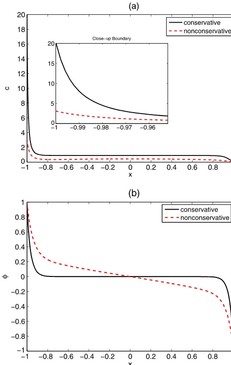
Fig. 3 Comparison between the simulation results from the mass-conservative and the non-conservative schemes for = 1,

η=4.63×10−5,φ₋=1,φ₊= −1,T =1. The calculations were performed witht=10−4andx=0.002. (a) The ion concentration profiles ofc2from the mass-conservative method (the solid line) and

the non-conservative method (the dashed line). (b) The corresponding electrostatic potentials

schemes (the solid lines) and the non-conservative schemes (the dashed lines). The parameters in the computations are the same as described in the previous Sect.4.2. To make fair comparison, all other aspects are kept same, including the time-step scheme (TR-BDF2), the discretization scheme for interior points of the domain, the initial condition, the phys-ical parameters, the time-step sizet and the space resolu-tionx. As shown in Fig.3(a), the ion concentration from the non-conservative scheme is substantially lower than that from the mass-conservative scheme and the variations near the boundaries are much smaller in the result from the non-conservative scheme. Furthermore, the electrostatic poten-tial obtained from the non-conservative scheme, shown in Fig. 3(b), has a linear profile with non-zero slope in the middle of the domain and much milder slopes at the

bound-Fig. 4 (a) The total ion concentration for species 2 as a function of time from the simulations using the mass-conservative (solid) and non– conservative (dashed) schemes. (b) The relative error in total concen-tration for both species. The parameters are identical to those in Fig.3

aries, when compared with that from the mass-conservative schemes.

Because of the no-flux boundary conditions (3a), the to-tal concentration of each ion species should be invariant in time. Figure4shows that the mass-conservative scheme pre-serves the conservation of the ions perfectly (up to the level of roundoff error) over a long period of time, while the total number of ions at the time t =1 obtained from the non-conservative scheme is reduced to less than half of the orig-inal amount.

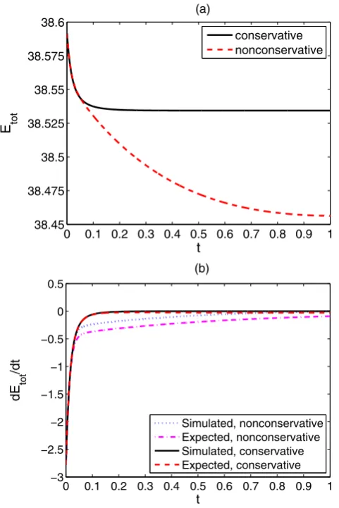
Fig. 5 (a) The total energy as a function of time from the simulations using the mass-conservative (solid) and non-conservative (dashed) schemes. (b) The rate of change in energy, dE

dt, obtained from the graph (a) and the right-hand side of Eq. (10). The solid and the dotted lines correspond to the left-hand side of Eq. (10) for the mass-conser-vative and the non-consermass-conser-vative schemes respectively. The dashed and the dash-dotted lines correspond to the right-hand side of Eq. (10) for the mass-conservative and the non-conservative schemes respectively. The parameters are identical to those in Fig.3

the non-conservative schemes (the dotted line) obtained by using a second-order finite difference based on the numer-ical resultE(t ) shown in Fig.5(a). In the same graph, we also plot the expected dissipation rate given by the right-hand side of (10), computed using the second-order central differencing and trapezoidal rule and shown by the dashed line for the conservative scheme and the dash-dotted line for the non-conservative scheme in Fig.5(b). It shows that the numerical result from the conservative scheme (the solid line) agrees with the energy dissipation law (the dashed line) very well. In contrast, the corresponding results for the non-conservative scheme show that the energy dissipation law is not satisfied after a short period of time. This is due to the fact that the total concentration from the non-conservative scheme displays very poor performance in conserving the

Fig. 6 The maximum rate of change in ion concentrations as a func-tion of time for the non-conservative (the dashed line) and conservative (the solid line) schemes. The parameters are identical to those in Fig.3

total concentrations. The results show that the discretization of the boundary conditions have profound impact on satis-fying the physical properties: the energy dissipation law and the conservation of the total number of ions.

In addition to energy decay, we compute the maximum rate of change in the concentrations of the species over the domain, i.e. maxi,−1≤x≤1|∂c_∂ti|. It is notable from the time derivative of concentration shown in Fig. 6 that the numerical results from the conservative numerical scheme steadily approach the equilibrium in time. On the other hand, the non-conservative scheme is approaching a steady state much faster initially, but, later in time, the non-conservative scheme’s behavior changes and it does not appear to reach a steady state. This result emphasizes the necessity of the conservative numerical scheme for long-time simulation.

4.4 Effect of parameters

The size of the difference in the results from conserva-tive and conservaconserva-tive schemes depends on the non-dimensional parameterχ2=ec0L

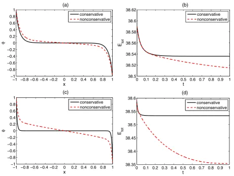
2

conser-Fig. 7 Comparison between the simulation results from the mass-conservative and the non-mass-conservative schemes for different values of the non-dimensional parameterχ2. (a) The electric potential for the

conservative and non-conservative schemes usingχ2=31.35. (b) The

total energy for the conservative and non-conservative schemes using

χ2=31.35. (c) The electric potential for the conservative and

non-conservative schemes usingχ2=501.60. (d) The total energy for the

conservative and non-conservative schemes usingχ2=501.60. The

calculations were performed witht=10−4 _{andx=0.001. The}

other parameters are identical to those in Fig.3

vative scheme in the energy plots of Fig.7(b) and (d). Com-paring the graphs of potential in Figs.3(a), (c) and7, we find that the value ofχ2primarily affects the width of the bound-ary layer, with largerχ2 resulting in thinner boundary lay-ers. A thinner boundary layer transitions much more sharply near the boundaries, and thus requires more computational grid points in the region and more truthful discretization of the boundary conditions. This causes the differences in elec-trostatic potential profiles and the energy dissipation in time (shown by Fig.7(b) and (d)) between the conservative and non-conservative schemes to be greater as one increasesχ2. A thinner boundary layer also affects performance with re-gard to the energy dissipation law, which is not shown here in plots. Largerχ2leads to a larger discrepancy between the decay rate of the total energy (the left-hand side of Eq.10) and the energy dissipation rate (the right-hand side of the law Eq.10), and this discrepancy gets worse faster for the non-conservative scheme than for the conservative scheme.

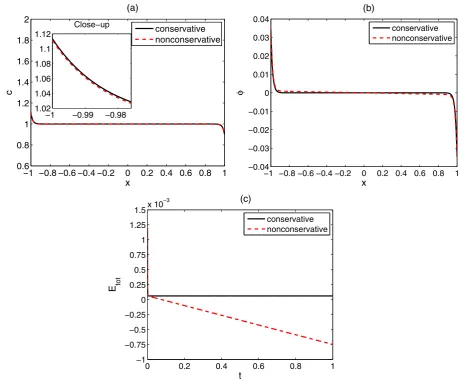
prop-Fig. 8 Comparison between the simulation results from the mass-conservative and the non-mass-conservative schemes forη=0.5. The other parameters are identical to those in Fig.3. (a) The ion concentration

of species 2 at the non-dimensionalized timeT=1. (b) The electric potential at the non-dimensionalized timeT=1. (c) The total energy as it varies in time

erty is shown in Fig.8. It appears that, forη=0.5, the to-tal energy from the non-conservative scheme decreases lin-early in time after an initial sharp drop, becoming negative at later time. On the other hand, the conservative scheme reaches a steady state very quickly and does not deviate from it. For small values ofηsuch as those shown in Fig.3, both the conservation property of the total concentrations and the energy dissipation law deteriorate at a fast pace for the non-conservative scheme, and the difference between the results from the conservative and the non-conservative schemes grows bigger asηgets smaller.

5 Conclusion

The primary objective of this work is to investigate the ef-fects of conservation property of discretization schemes on the numerical results. We have shown that, with regard to

the PNP equations, whether a numerical method preserves the mass conservation could have a critical impact on the behavior of the system, especially the steady state results. We have provided a discretization scheme that preserves the mass conservation exactly (excluding the round-off errors) and the energy dissipation law well for long-time simula-tion.

Our method is implicit in time and second-order accurate in both space and time. We have verified that approximat-ing the fully implicit solution is necessary for second-order convergence in time. Further, we find that one can avoid us-ing Newton-type nonlinear solvers by performus-ing a simple iterative scheme.

Further, we have derived the conditions on the proposed numerical scheme under which it will preserve the positivity of the concentrations.

of the non-dimensional parametersχ2in the Poisson equa-tion andηin the Robin boundary condition for the electro-static potential. We find that the mass-conserving scheme is more robust to changes in parameters, especially changes to the value ofη.

Although this work makes good progress in constructing an accurate method for solving the Poisson–Nernst–Planck equations numerically, there are many challenges remaining. First, one of them is to account for the finite size of the ions as its effect is enormous considering the narrow width of the ion channels [17,19]. Second, for most ion channels, the appropriate boundary conditions are Dirichlet-type. We will investigate the possibility to preserve the energy dissipation law exactly instead of the mass and study the effect of the conservation on long-term behavior of the simulation. Third, we would like to include distributions of permanent charges for studying selectivity of ion channels.

Acknowledgements X. Li is partially supported by the NSF grant DMS-0914923 and C. Liu is partially supported by the NSF grants DMS-1109107, DMS-1216938 and DMS-1159937.

References

1. Bank, R.E., Coughran, W.M. Jr., Fichtner, W., Grosse, E.H., Rose, D.J., Smith, R.K.: Transient simulation of silicon devices and circuits. IEEE Trans. Comput.-Aided Des. Integr. Circuits Syst. CAD-4, 436–451 (1985)

2. Bolley, C., Crouzeix, M.: Conservation de la positivité lors de la discrétisation des problèmes d’évolution paraboliques. Modél. Math. Anal. Numér. 12(3), 237–245 (1978)

3. Cagni, E., Remondini, D., Mesirca, P., Castellani, G., Verondini, E., Bersani, F.: Effects of exogenous electromagnetic fields on a simplified ion channel model. J. Biol. Phys. 33, 183–194 (2007) 4. Celledoni, E., Grimm, V., McLachlan, R., McLaren, D., O’Neale,

D., Owren, B., Quispel, G.: Preserving energy resp. dissipation in numerical pdes using the “average vector field” method. J. Com-put. Phys. 231, 6770–6789 (2012)

5. Chiu, E., Wang, Q., Hu, R., Jameson, A.: A conservative mesh-free scheme and generalized framework for conservation laws. SIAM J. Sci. Comput. 34, A2896–A2916 (2012)

6. Domene, C., Vemparala, S., Furini, S., Sharp, K., Klein, M.: The role of conformation in ion permeation in a k+ channel. J. Am. Chem. Soc. 130 (2008)

7. Doyle, D., Cabral, J.M., Pfuetzner, R., Kuo J. G, A., Cohen, S., Chait, B., MacKinnon, R.: The structure of the potassium chan-nel: molecular basis of K+conduction and selectivity. Science 280 (1998)

8. Eisenberg, R.: Ion channels in biological membranes: electrostatic analysis of a natural nanotube. Contemp. Phys. 39, 447 (1998) 9. Fisher, T., Carpenter, M., Nordström, J., Yamaleev, N., Swanson,

C.: Discretely conservative finite-difference formulations for non-linear conservation laws in split form: theory and boundary condi-tions. J. Comput. Phys. 234, 353–375 (2012)

10. Gardner, C., Jones, J.: Electrodiffusion model simulation of the potassium channel. J. Theor. Biol. 291, 10–13 (2011)

11. Gardner, C., Nonner, W., Eisenberg, R.: Electrodiffusion model simulation of ionic channels: 1d simulations. J. Comput. Electron. 3, 25–31 (2004)

12. Gillespie, D.: Energetics of divalent selectivity in a calcium chan-nel: the ryanodine receptor case study. Biophys. J. 94, 1169–1984 (2008)

13. Gillespie, D., Nonner, W., Eisenberg, R.: Coupling Poisson– Nernst–Planck and density functional theory to calculate ion flux. J. Phys. Condens. Matter 14, 12,129–12,145 (2002)

14. Ham, F., Lien, F., Strong, A.: A fully conservative second-order finite difference scheme for incompressible flow on nonuniform grids. J. Comput. Phys. 177, 117–133 (2002)

15. Harlow, F.H., Welch, J.E.: Numerical calculation of time-dependent viscous incompressible flow of fluid with free surface. Phys. Fluids 8, 2182 (1965)

16. Hof, B., Veldman, A.: Mass, momentum and energy conserving (mamec) discretizations on general grids for the compressible Eu-ler and shallow water equations. J. Comput. Phys. 231, 4723–4744 (2012)

17. Horng, T., Lin, T., Liu, C., Eisenberg, B.: PNP equations with steric effects: a model of ion flow through channels. J. Phys. Chem. B 116, 422–441 (2012)

18. Hundsdorfer, W., Verwer, J.: Numerical Solution of Time-Dependent Advection-Diffusion-Reaction Equations. Springer Series in Computational Mathematics. Springer, Berlin (2003) 19. Hyon, Y., Eisenberg, R., Liu, C.: A mathematical model for the

hard sphere repulsion in ionic solutions. Commun. Math. Sci. 9, 459–475 (2011)

20. Kajishima, T.: Finite-difference method for convective terms using non-uniform grid. Trans. Jpn. Soc. Mech. Eng. C 65-633(Part B), 1607–1612 (1999)

21. Lee, C., Lee, H., Hyon, Y., Lin, T., Liu, C.: New Poisson– Boltzmann type equations: one-dimensional solutions. Nonlinear-ity 24, 431 (2011)

22. Li, S., Vu-Quoc, L.: Finite difference calculus invariant structure of a class of algorithms for the nonlinear Klein–Gordon equation. SIAM J. Numer. Anal. 32, 1839–1875 (1995)

23. Lopreore, C., Bartol, T., Coggan, J., Keller, D., Sosinsky, G., Ellisman, M., Sejnowski, T.: Computational modeling of three-dimensional electrodiffusion in biological systems: application to the node of ranvier. Biophys. J. 95, 2624–2635 (2008)

24. Markowich, P., Ringhofer, C., Schmeiser, C.: Semiconductor Equations. Springer, Berlin (1990)

25. Morinishi, Y., Lund, T., Vasilyev, O., Moin, P.: Fully conserva-tive higher order finite difference schemes for incompressible flow. J. Comput. Phys. 143(1), 90–124 (1998)

26. Morinishi, Y., Vasilyev, O., Ogi, T.: Fully conservative finite dif-ference scheme in cylindrical coordinates for incompressible flow simulations. J. Comput. Phys. 197, 686–710 (2004)

27. Nanninga, P.M.: A computational neuron model based on Poisson–Nernst–Planck theory. In: Mercer, G.N., Roberts, A.J. (eds.) Proceedings of the 14th Biennial Computational Techniques and Applications Conference, CTAC-2008, ANZIAM J, vol. 50, pp. C46–C59 (2008)

28. Neuen, C.: A multiscale approach to the Poisson–Nernst–Planck equation. Diploma Thesis, University of Bonn, Germany (2010) 29. Qiao, Z., Zhang, Z., Tang, T.: An adaptive time-stepping strategy

for the molecular beam epitaxy models. SIAM J. Sci. Comput. 33(3), 1395–1414 (2011)

30. Teorell, T.: Transport processes and electrical phenomena in ionic membranes. Prog. Biophys. Mol. Biol. 3, 305 (1953)

31. Vasilyev, O.V.: High order finite difference schemes on non-uniform meshes with good conservation properties. J. Comput. Phys. 157(2), 746–761 (2000)

32. Wei, G.W., Zheng, Q., Chen, Z., Xia, K.: Variational multiscale models for charge transport. SIAM Rev. 54, 699–754 (2012) 33. Zhang, Z., Qiao, Z.: An adaptive time-stepping strategy for the