Northern elephant seals adjust gliding and stroking patterns with changes in buoyancy: validation of at sea metrics of body density

INTRODUCTION

Many marine divers, such as phocid seals, undergo substantial changes in body mass and condition as they mature as well as over their annual fasting and foraging cycles (Crocker et al., 1997; Biuw et al., 2003). In capital breeding phocids, resources used during fasting periods associated with breeding and moult are replenished while animals feed at sea between these fasting periods (Costa, 1993). The size of the stores reflects an integration of foraging effort (energy expenditure) and foraging success (energy assimilation). For seals that breed on land, researchers have been able to quantify the consequences of variation in these resources on future survival and reproductive success (Arnbom et al., 1993; Costa, 1993; Fedak et al., 1996; Arnbom et al., 1997; Pomeroy et al., 1999; McMahon et al., 2000; Crocker et al., 2001b; Hall et al., 2001). This has traditionally been accomplished by measuring animal mass combined with determination of water content using isotope dilution techniques (Pace and Rathbun, 1945; Reilly and Fedak, 1990; Arnould, 1995; Bowen and Iverson, 1998). If such measurements are obtained prior to departure from and again upon return to land,

these approaches are extremely useful for determining the net acquired resources integrated over the entire feeding period at sea, and the resources available for onshore process such as breeding and moult. Similarly, if measurements are again obtained prior to the next departure, they permit estimation of the resource utilization of these processes over the time spent on land (Anderson et al., 1993; Costa, 1993). However, these methods cannot be used to map where and when animals are gaining or losing resources as they cannot be applied to free-ranging animals at sea.

Measurements of resource acquisition by animals while at sea are important for understanding how they manage their energy budgets to cover various life history requirements associated with growth and reproduction. But these measurements are also important more generally for understanding foraging ecology and ecosystem interactions, and for management decisions regarding marine species and ecosystems. There are a variety of approaches to estimate where and when marine animals are likely to be feeding, ranging from measurements derived from surface tracks [i.e. transit rate first passage time, fractal landscape, state space models (Fauchald and The Journal of Experimental Biology 214, 2973-2987

© 2011. Published by The Company of Biologists Ltd doi:10.1242/jeb.055137

RESEARCH ARTICLE

Northern elephant seals adjust gliding and stroking patterns with changes in

buoyancy: validation of at-sea metrics of body density

Kagari Aoki

1,2

_{, Yuuki Y. Watanabe}

3

_{, Daniel E. Crocker}

4

_{, Patrick W. Robinson}

5

_{, Martin Biuw}

1,6

_,

Daniel P. Costa

5

, Nobuyuki Miyazaki

7

, Mike A. Fedak

1

and Patrick J. O. Miller

1,

*

1_{Sea Mammal Research Unit, Scottish Oceans Institute, University of Saint Andrews, Saint Andrews, Fife KY16 8LB, UK,} 2_{International Coastal Research Centre, Atmosphere and Ocean Research Institute, The University of Tokyo, 2-106-1 Akahama,}

Otsuchi, Iwate 028-1102, Japan, 3_{National Institute of Polar Research, 10-3, Midoricho, Tachikawa, Tokyo 190-8518, Japan,} 4_{Department of Biology, Sonoma State University, Rohnert Park, CA 94928, USA,} 5_{Long Marine Laboratory, Department of Ecology}

and Evolutionary Biology, University of California, Santa Cruz, CA 95064, USA, 6_{Norwegian Polar Institute, Polar Environmental} Centre, 9296 Tromsø, Norway and 7_{Center for International Cooperation, Ocean Research Institute, The University of Tokyo,}

1-15-1Minamidai, Nakano-ku, Tokyo 164-8639, Japan

*Author for correspondence ([email protected])

Accepted 31 May 2011

SUMMARY

Many diving animals undergo substantial changes in their body density that are the result of changes in lipid content over their annual fasting cycle. Because the size of the lipid stores reflects an integration of foraging effort (energy expenditure) and foraging success (energy assimilation), measuring body density is a good way to track net resource acquisition of free-ranging animals while at sea. Here, we experimentally altered the body density and mass of three free-ranging elephant seals by remotely detaching weights and floats while monitoring their swimming speed, depth and three-axis acceleration with a high-resolution data logger. Cross-validation of three methods for estimating body density from hydrodynamic gliding performance of freely diving animals showed strong positive correlation with body density estimates obtained from isotope dilution body composition analysis over density ranges of 1015 to 1060kgm–3. All three hydrodynamic models were within 1% of, but slightly greater than, body density measurements determined by isotope dilution, and therefore have the potential to track changes in body condition of a wide range of freely diving animals. Gliding during ascent and descent clearly increased and stroke rate decreased when buoyancy manipulations aided the direction of vertical transit, but ascent and descent speed were largely unchanged. The seals adjusted stroking intensity to maintain swim speed within a narrow range, despite changes in buoyancy. During active swimming, all three seals increased the amplitude of lateral body accelerations and two of the seals altered stroke frequency in response to the need to produce thrust required to overcome combined drag and buoyancy forces.

Supplementary material available online at http://jeb.biologists.org/cgi/content/full/214/17/2973/DC1

Tveraa, 2003; Jonsen et al., 2005; Tremblay et al., 2007; Patterson et al., 2008)] to variations in the diving pattern (Mori, 1998; Bailleul et al., 2008). However, none of these methods provide a measure of food intake and, depending on the animals’ foraging strategies and movement patterns, they may miss or over-represent foraging (Robinson et al., 2010). Methods using a variety of sensors to measure actual food intake or prey capture events have also been developed (e.g. Wilson et al., 1992; Austin et al., 2006; Robinson et al., 2007; Kuhn et al., 2008; Suzuki et al., 2009). Although these methods are quite useful to provide timing of feeding and prey encounter rates, they do not quantify resource acquisition, which is represented as the balance between energetic expenditure and energetic intake from prey ingestion.

One alternative approach to estimating foraging success of seals while at sea is based on monitoring changes in their body density as a proxy for lipid content (Crocker et al., 1997; Webb et al., 1998; Biuw et al., 2003), and this approach provides a means to identify advantageous foraging locations (Biuw et al., 2007; Robinson et al., 2010). The rationale behind this approach is that lipid, the main energy reserve in seals, is less dense than seawater whereas non-lipid compartments are slightly more dense than seawater (Moya-Laraño et al., 2008), and changes in relative body composition will therefore influence overall body density and thereby the total forces acting on a diving animal (Fedak et al., 1994; Crocker et al., 1997; Webb et al., 1998; Biuw et al., 2003). Commonly, the term ‘buoyancy’ is used to refer to the net immersed weight of a body (Beck et al., 2000; Williams et al., 2000) (see Eqn 7). Buoyancy acts vertically, adding to (or subtracting from) drag forces during transit to and from depth (Webb et al., 1998; Beck et al., 2000), and can exceed drag forces at typical travel speeds for many divers. Buoyancy forces have been shown to influence the stroking patterns of swimmers, with increased gliding when buoyancy aids movement (Skrovan et al., 1999; Williams et al., 2000; Miller et al., 2004). Buoyancy forces also modulate the rate of drift during inactive drifting periods (Crocker et al., 1997; Webb et al., 1998; Biuw et al., 2003) and prolonged glides, with higher speeds obtained when buoyancy aids the glide (Watanabe et al., 2006). In stroke-and-glide swimming, buoyancy alters the rate of deceleration (or acceleration) during gliding phases (Miller et al., 2004).

Because of buoyancy’s effect on gliding performance, tissue density of a wide range of diving animals (including seals and whales) can potentially be estimated from hydrodynamic analysis of terminal drift (Biuw et al., 2003) or terminal glide speeds (Watanabe et al., 2006), as well as deceleration (or acceleration) rates during glides (Miller et al., 2004). One caveat associated with the use of body density to track changes in foraging success is that it can only be used to estimate changes in the relative body composition, whereas in reality body changes associated with feeding or non-feeding will also change the overall body mass of the animal. It is also possible that resources acquired while feeding are allocated to lean tissue growth rather than the accumulation of lipid energy reserves, leading to an increase in body density. Measuring changes of body mass of freely diving animals would be helpful, but is likely to be more challenging than measuring changes in body density. However, an observed decrease in body density most likely represents the accumulation of lipid reserves, and should therefore provide a conservative indicator of foraging success.

There is also substantial interest in how animals alter their patterns of gliding and active swimming in response to changes in buoyancy. Some longer-term changes in ascent and descent rates appear to correlate with fat content (Webb et al., 1998; Beck et al., 2000). Extensive use of gliding indicates that animals modulate their overall

glide and stroke patterns in order to maintain a preferred ascent or descent speed (Thompson et al., 1993) on a dive-by-dive basis. Another factor is that propulsive efficiency of thrusting organs are thought be greatest within a narrow range of Strouhal numbers (fD/U; where fis stroke frequency, Dis stroke amplitude and Uis forward speed) (Taylor et al., 2003). Thus, animals may have particular biomechanical strategies to maintain propulsive efficiency in changing conditions. During active thrusting periods, the amount of thrust generated could be modulated by altering stroke frequency (Lovvorn et al., 1999; Lovvorn et al., 2004) – defined as the oscillation rate of thrusting during active swimming – stroke amplitude and/or flipper speed (Fish, 1993). In fact, flipper speed and/or stroke amplitude may be fundamentally linked to stroke cycle duration. Though some captive studies have suggested that seals alter stroke cycle frequency rather than amplitude (e.g. Fish, 1988), others have reported that stroke amplitude variations are also important (e.g. Wilson and Liebsch, 2003).

In this study, we experimentally manipulated the body density and mass of instrumented free-diving Northern elephant seals,

Mirounga angustirostris (Gill 1866), to explore from both an

ecological and biomechanical perspective how gliding and stroking patterns are altered by changes in buoyancy forces acting on them. Weights, and in one case a weight and a float, were sequentially released from translocated Northern elephant seals (Oliver et al., 1998) during their return to Anõ Nuevo State Reserve (San Mateo County, CA, USA). These different density and mass manipulation conditions encompassed a wide range of body densities of ecological relevance. We describe how the different density conditions relate to time spent gliding, descent and ascent transit speeds, lateral stroke cycle frequency and lateral dynamic acceleration during ascent and descent. During stroking, we estimate thrust produced by combining drag and buoyancy forces, and relate the thrust to stroke cycle frequency and amplitude of lateral dynamic acceleration. Though it is difficult to measure stroke amplitude directly in free-diving animals, accelerometers record dynamic acceleration of the body, which is oscillated laterally when seals produce thrust (Sato et al., 2003). The amplitude of dynamic body acceleration has been shown to relate to metabolic rate in a diving seabird (Wilson et al., 2006). However, it remains unclear precisely how the amplitude of acceleration might relate to the amplitude of stroking or flipper speed throughout a stroke. We consider that the amplitude of lateral acceleration should be an indicator of thrusting intensity, possibly also reflecting stroke amplitude.

An important goal of our study is to cross-validate three published methods for directly estimating body density from hydrodynamic gliding performance: terminal drift rate (Biuw et al., 2003), deceleration during glides (Miller et al., 2004) and terminal gliding speed (Watanabe et al., 2006). We will also compare the estimates from these methods with body density calculated using the isotope dilution method. The hydrodynamic performance methods have separately been shown to work with different free-ranging species (Biuw et al., 2003; Miller et al., 2004; Watanabe et al., 2006), but have not been evaluated from the same data set on the same species. This set of hydrodynamic gliding methods to estimate body density can be applied to a wide range of diving species and opens new avenues to track the body condition of free-ranging animals and to determine where and when they gain resources.

MATERIALS AND METHODS Field experiments

standard protocols (Le Boeuf et al., 1988; Le Boeuf et al., 2000) and transported to Long Marine Laboratory (Santa Cruz, CA, USA) where they were held overnight for measurement, sample collection and instrument attachment. Body mass, maximum girth and length (standard length L, i.e. the straight line between the tip of the nose and the tip of the tail) were measured (Table1). Body condition was measured for each seal using water isotope dilution (see Body density measured from isotope dilution methods). Each multi-sensor data logger (W2000-3MPD3GT; 26mm diameter, 175mm length, 140g in air; Little Leonardo Co., Bunkyo-ku, Tokyo, Japan), weight and float was attached to the fur on the back of the seal using nylon mesh and Loctite®_{Quick Set}TM_{Epoxy (for details see}

Experimental manipulation of body density). The logger was set to record depth, swim speed and temperature at 1s intervals, and three-dimensional accelerations (for detecting pitch and hind flipper movements) at 1/16s intervals, with a memory of 512Mb. The measurement range of the depth sensor of the data logger was 0–2000m with a resolution of 0.5m. The seals were then transported by boat to a release site above the Monterey submarine canyon (36.6°N, 122.5°W), approximately 45km southwest of Año Nuevo State Reserve. The three seals (seals 1, 2 and 4) returned to the Año Nuevo colony within 2days and their instruments were recovered (Table1). We could not recapture one of the seals (seal 3) and did not recover the instrument.

Experimental manipulation of body density

We experimentally changed the body density of our animals by attaching a cuboid weight (3.63kg in air) and a round float (2.28kg in air) just behind the data logger on the seal’s back. The float was covered with a streamlined plastic housing to provide a consistent alteration in frontal area for each seal. The volume of the float was adjusted so that the float and the weight together were neutrally buoyant in seawater. For seals 1 and 4, we used a time-scheduled release mechanism (Little Leonardo Co.) to automatically release the weight and float 8 and 16h after deployment, respectively. The release order was switched for seal 2, so the float and then weight were scheduled to be automatically detached 8 and 16h after deployment, respectively. This allowed us to obtain three buoyancy manipulation conditions: floated-and-weighted (float and weight attached), weighted (only weight attached) and floated (only float attached).

Body density measured with gravity-based isotope dilution methods

We estimated the body composition prior to the release of each seal by isotope dilution. Each animal was given an intraperitoneal injection of ~7.4MBq of tritiated water (3_{HHO). After a minimum}

of 3h equilibration, a blood sample was taken to determine the specific activity of body water (Costa et al., 1986; Costa, 1987). Injection syringes were gravimetrically calibrated to determine precise injection volumes. Serum samples were collected using freeze trap distillation and counted in 7ml Betaphase scintillation

cocktail on a Beckmann LS6500 scintillation counter (Ortiz et al., 1978). Total body water (TBW; kg) was calculated from the isotopic dilution space (3_{HHOspace) using the equation developed for grey}

seals (Reilly and Fedak, 1990):

TBW–0.234 + 0.971(3_{HHOspace). (1)}

The proportion of the total amount of lipid (%TBL) and protein (%TBP) to body mass (kg) and total body ash (TBA; kg) were also calculated (Reilly and Fedak, 1990):

%TBL105.1 – 1.47(%TBW), (2) %TBP0.42(%TBW) – 4.75, (3) TBA0.1 – 0.008mseal+ 0.05TBW, (4)

where msealis the body mass of the seal and %TBW is the proportion

of TBW to body mass (kg). Total body density of the seal (seal)

was calculated from the proportion (P) and the density () of each component following Biuw et al. (Biuw et al., 2003):

seal lPl+ pPp+ aPa+ bwPbw, (5)

where the subscripts l, p, a and bw refer to lipid, protein, ash and body water, respectively. We used the following density values: l900.7, p1340, a2300 and bw994kgm–3, which are reported

for humans (Moore et al., 1963) (cited from Biuw et al., 2003). The body density of animals for each buoyancy manipulation condition (i.e. floated-and-weighted, weighted and floated conditions) was calculated as:

where the volume of the seal (m3_{) is V}

sealmseal/seal, mattachment(kg)

is the mass of a lead weight and/or the float and Vattachment(m3) is

the volume of a lead weight and/or the float.

Time series data analysis for body density models and stroking patterns

Diving data recorded from the data loggers were analyzed using the software IGOR Pro (WaveMetrics Inc., Lake Oswego, OR, USA). The start and end of dives were defined as seals descending below and ascending above a depth of 2m, respectively. All deep dives (maximum depth >100m) were divided into three phases: (1) descent phase (from the start of a dive to the first time at which the depth change rate was negative); (2) ascent phase (from the last time at which the depth change rate was positive to the end of the dive); and (3) bottom phase (the time between the end of the descent phase and the beginning of the ascent phase).

Accelerations in three axes (longitudinal, lateral and dorso-ventral) measured by the logger can be broken into components related to the orientation of the animal with respect to gravity (static components) and dynamic accelerations imposed by the flippers’

ρseal, manipulation= m_Vseal+mattachment seal+Vattachment

, (6)

Table1. Summary of study animals and experimental body density manipulation

IDa _{Sex Length}b_{(m) Body mass (kg) Girth (m) Total tagged duration (h) Experimental manipulation of body density}c

Seal 1 Female 1.74 161 1.48 38.6 Weighted, unattached

Seal 2 Male 1.75 162 1.46 70.4 Floated-and-weighted, floated, unattached

Seal 4 Unknown 1.89 193 1.56 31.9 Weighted, unattached

a_{Seal 3 was not recaptured and we could not recover the instrument.}

thrust (dynamic components). Lower-frequency gravity-based acceleration of the longitudinal axis was used to calculate the pitch angle of animals () (Sato et al., 2003; Watanabe et al., 2006). This acceleration was extracted from the raw acceleration data using the low-pass filter at 0.50, 0.50 and 0.40Hz for seals 1, 2 and 4, respectively, using the software IFDL within IGOR Pro. The frequency boundary for the filter was determined for each seal by calculating the power spectral density of the lateral axis acceleration data using a fast Fourier transformation within IGOR Pro. In all cases, the power spectral density showed a clear trough, which is considered to represent the boundary between gravity-based and dynamic acceleration components (Sato et al., 2007). Negative pitch indicates descent whereas positive pitch represents ascent. The pitch was adjusted for possible off-axis placement on the body by using the cumulative value method (Sato et al., 2003). Higher-frequency dynamic acceleration of the lateral axis was obtained by subtracting the low-frequency components from the raw acceleration data to identify individual strokes. The peaks and troughs of the signal with absolute amplitudes greater than a specified threshold were considered to represent individual strokes (Sato et al., 2003). To select the threshold, we made histograms of absolute amplitudes from all peaks and troughs for each seal. This analysis showed a clear boundary between small noise signals and strokes. We defined the boundary as the threshold (1.27, 0.39, 0.59ms–2_{for seals 1, 2}

and 4, respectively). An entire peak–trough cycle corresponds to a two flipper strokes (i.e. left–right and right–left).

Speed through the water was measured by an external propeller on the data logger. After analyzing acceleration data, the rotation rate (revolutionss–1_{) of the propeller was converted into swim speed}

(ms–1_{) using a calibration line for each seal (Sato et al., 2003). The}

calibration line was obtained from a linear regression of rotation rate against swim speed (ms–1_{), which was calculated from averaged}

rate of vertical depth change divided by the averaged sine of the pitch at 5s intervals when the averaged sine of the pitch was greater than 0.8 (for details, see Sato et al., 2003). The regression coefficient values were 0.940, 0.877 and 0.966 for seals 1, 2 and 4, respectively. The corresponding swim speed resolution was 0.035, 0.032 and 0.033ms–1_{for seals 1, 2 and 4, respectively.}

Body density models

The body density of the animals was estimated by using three different hydrodynamic models: a drift-dive model (Biuw et al., 2003), a glide model (Miller et al., 2004) and a prolonged-glide model (Watanabe et al., 2006). All three models quantify the influence of hydrodynamic drag and buoyancy on a passively moving body. Here, buoyancy is defined as the difference between the body density of the animal and that of the surrounding seawater (Lovvorn and Jones, 1991; Beck et al., 2000):

FB(sw– seal)Vsealg, (7)

where FBis buoyancy force (N), sw is the density of seawater

(kgm–3_{) and gis gravity. The drag of the seal during drifts and}

glides was calculated as:

FD0.5CdswAU2_{, (8)}

where FDis drag force (N), Cdis the drag coefficient, Ais frontal

or surface area of the seal (m2_{) and Uis swim speed (ms}–1_).

Drift-dive model

We selected drift dives based upon the criteria used by previous studies (Biuw et al., 2003; Mitani et al., 2009). Drift dives include a rapid descent phase (U1) followed by a prolonged phase of slower

descent or ascent (U2), followed by a rapid ascent to the surface

(U3) (see fig.1 in Biuw et al., 2003). Drift dives were defined as

dives where U2had no active stroking and constantly low depth

change rate (mean <0.5ms–1_{), with continuous descent or ascent}

and continuously low swim speed (mean <0.5ms–1_).

In drift phases (i.e. U2), the absolute buoyancy force is assumed

to equal the drag force at terminal speed (Biuw et al., 2003). Therefore, the theoretical drift rate Udrift(ms–1) is calculated as the

terminal speed by FDFBduring ascending drift phases and FD–FB

during descending drift phases. Udriftfor descending drift phases is

shown as:

where mis the total mass of the seal (kg), ASis surface area (m2)

and Cd,s is the drag coefficient based on total surface area (0.69)

(Biuw et al., 2003). Total body mass was calculated as msealme, where meis a multiplier for entrained water adhering to the surface of the

seal. The value for mewas set to 1.06 based on the measure for a

prolate spheroid with a fineness ratio of 5.0 (Skrovan et al., 1999; Miller et al., 2004). ASwas calculated based on the assumption that

the seal is two opposing cones with a base that corresponds to total girth (modified from Bell et al., 1997). The anterior cone was assumed to have a height corresponding to one-third of the standard length L, whereas the posterior cone had a height of two-thirds of

L. We assume that Udriftwould correspond to the depth change rate

(ms–1_{) during the drift phase. The depth change rate and } swwere

averaged during the drift phase. sealwas estimated for each dive.

Glide model

During glides, acceleration along the swimming path was determined by the difference between drag force (FD) and buoyancy force (FB)

parallel to the swimming path: maFBsin–FD(Miller et al., 2004).

The acceleration is therefore given by:

where ais the acceleration (ms–2_{) observed during the glide, C} d,f

is the drag coefficient based on frontal area (see Calculation of Cd

for prolonged-glide and glide models) and Afis the frontal area (m2)

of the seal. Afwas calculated from the girth measurement, assuming

that seals are circular in cross-section.

We conducted this analysis for glides selected by the following three criteria. First, we selected glides where absolute pitch, ascending or descending, averaged more than 30deg, because the effect of buoyancy should be more evident when the magnitude of buoyancy is weighted by more than sin(30deg) (Watanabe et al., 2006). Second, to select stable glides, we excluded glides that had rapid changes in pitch (greater than the mean ± s.d. change rate during all dives: 7, 4 and 5degs–1_{for seals 1, 2 and 4, respectively)}

because deceleration would be caused by the animal’s movement. Third, glides that had continuous decreasing or increasing changes in swim speed were selected to exclude unstable glides. Acceleration was measured using a linear regression line of speed vstime. , sw

and Uwere averaged during each glide period. These analyses were conducted at 5s intervals. To increase the range of glide speed, prolonged glides were divided into multiple sub-glides at 5s intervals (Miller et al., 2004). Only data from every 10s interval were used to reduce potential autocorrelation of the data. sealwas

determined by non-linear least-squares methods during each attachment condition for each seal.

a= −Cd,fAf

m 0.5ρswU2+(ρsw/ρseal−1)gsinθ , (10)

Udrift= (1− ρsw/ρseal)m

g

0.5Cd,sρswAS

Prolonged-glide model

In prolonged-glide phases, drag equals the magnitude of buoyancy weighted by sinat terminal speed: FDFBsin(Watanabe et al.,

2006). The theoretical terminal speed (Uter) is then calculated by:

This equation includes two unknown quantities: sealand Uter. We

simulated Uter at various possible seal values within the range

1000–1080kgm–3_{, using pitch measured every second. The}

simulated speed was then compared with the measured speed. seal

was determined by least-squares methods for each dive. Similar to the glide model described above, this analysis was conducted for dives where the average absolute value of pitch exceeded 30deg during descents or ascents, which included prolonged glides.

For this analysis, we predicted the gliding duration required for each individual to achieve terminal speed (Fig.1) because swim speed at the beginning of a prolonged-glide may not represent the terminal speed (Watanabe et al., 2006). This simulation was conducted based on our analyzing criteria (||>30deg) and the body density estimated from isotope dilution method (Table2). First, we calculated theoretical terminal speed from Eqn 11. Second, we simulated changes in swim speed from glide start speed to theoretical terminal speed using the glide model. Eqn 10 of the glide model was rewritten as:

where Ut+1and Utare swim speeds (ms–1) at times t+1 and t(s), respectively. Glide start speed (U0) was set as 0.5–2.0m s–1based

Uter=

(ρsw/ρseal−1)mgsinθ 0.5Cd,fρswAf

. (11)

Ut+1=Ut−Cd,f_mAf0.5ρswU2+(ρsw/ρseal−1)gsinθ , (12)

upon our observations of the seals’ speeds. U0was substituted as Utto calculate U1, and then the U1was substituted as Utto calculate

U2 (i.e. Ut+1). Therefore, this equation allows us to calculate

changes in swim speed from glide start speed at 1s intervals. Finally,

Ut+1(t+1 is the predicted time to reach terminal speed) was assumed

to be theoretical terminal speed Uter when it was within 1.0% of Uter. This simulation was conducted for each experimental condition

for each seal.The predicted time to reach terminal speed ranged from 12 to 36s for our animals (Fig.1) and increased with smaller differences in density between the seal and surrounding seawater. We excluded speed data measured at the beginning of the prolonged glide (40s) because the measured speed might not have reached terminal speed.

The influence of depth for all body density models The total buoyancy of an air-breathing aquatic animal changes with depth owing to residual air in the lungs. This residual air could affect our estimation of seal, but this effect is reduced at

greater depths because air volume decreases with increasing depth following Boyle’s law (Biuw et al., 2003). To minimize the effect of gases on buoyancy, we only used data from depths greater than 100m.

Because buoyancy is a function of the difference between the density of the animal and seawater, changes in seawater density with depth could substantially affect our estimation of seal (see

Miller et al., 2004). Therefore, the density of seawater was estimated at 1s intervals from depth (m) and temperature (°C), measured by the data loggers, and salinity estimates of 34.84‰ (Vogel, 1994) using the International Equation of State of Seawater (UNESCO, 1981). Water temperature at depths greater than 100m ranged from 5.1 to 10.7°C, and the corresponding density of the seawater ranged between 1027.2 and 1030.8kgm–3_.

Calculation of Cdfor prolonged-glide and glide models

Gliding seals should swim head first to maximize their movement efficiency by minimizing drag. Therefore, the drag coefficient during glides would be different from that of drift phases, during which the body orientation is more like a falling leaf (Mitani et al., 2009), for which we used a surface area drag coefficient of 0.69 (Biuw et al., 2003). Drag force during glides was calculated from the deceleration rate during horizontal gliding: FDma (Bilo and

Nachtigall, 1980; Williams and Kooyman, 1985; Feldkamp, 1987; Watanabe et al., 2006). Cd,fis therefore given by:

Cd,f2m(Ut– Ut+1) / (swAfU2), (13)

where Utand Ut+1were averaged to give mean glide speed (U; ms–1);

sw was also averaged during these periods. We extracted 50

deceleration phases for each experimental condition of each seal when the seals swam horizontally (i.e. depth changes are zero) using stroke-and-glide patterns during the bottom phases of dives.

Eqn 13 can be rewritten as:

Therefore, by using horizontal glides to estimate the constant on the left-hand side of Eqn 14, it is possible to calculate body density using the prolonged-glide and glide models even without specific information on body mass and reference surface area.

The drag coefficient was recorded along with the Reynolds number (Re): ReLU/, where  is the kinematic viscosity of seawater (1.35⫻10–6_m2_s–1_{) (Lide, 2003). We estimated C}

d,f at

293±63, 183±102 and 157±55m for seals 1, 2 and 4, respectively.

Cd,fAf

m =2(Ut −Ut+1) / (ρswU2) . (14) 2.0

1.8

1.6

1.4

1.2

1.0

0.8

0.6

0.4

S

wim

s

peed (m

s

–1)

60 50 40 30 20 10 0

Elapsed time (s)

Pitch angle, 90 deg

Pitch angle, 30 deg

Speed predicted from glide model, pitch 90 deg

Speed predicted from glide model, pitch 30 deg

Terminal speed predicted from the prolonged-glide model

Glide start, 0.5 m s–1 Glide start, 2.0 m s–1

Because we cannot assume that the seals were neutrally buoyant at these depths, the seals should produce lift to maintain their horizontal motion. We specifically address the potential influence of lift on our analyses in the Appendix.

Stroking patterns

Stroke rate (s–1_{) during descent and ascent was calculated from the}

total number of strokes divided by the duration of each phase for each dive. The amplitude of lateral acceleration (ms–2_{) was}

considered to be a relative indicator of stroke intensity and was expected to be associated with stroke amplitude (m). The amplitude of lateral acceleration was quantified as half of the peak-to-peak recorded values. Amplitude of lateral acceleration was averaged over each phase for each dive during descent and ascent. These analyses were conducted for all deep dives (maximum depth >100 m)

To investigate the effects of buoyancy in relation to swim speed and stroke patterns, we estimated propulsive force while our animals swam actively. The propulsive force of the animals should equal resistance force (FR), including drag and buoyancy at times when

speed is constant (Lovvorn et al., 2004). The resistance force is calculated by FRFD+FBsin from Eqns 7, 8 and 11. For this

analysis, we used the body density calculated using the isotope dilution method. The term  is the active-to-passive drag ratio. Studies of captive phocid seals and dolphins suggested that actively swimming animals had higher drag than gliding animals (Williams and Kooyman, 1985; Fish, 1988; Fish, 1993). However, hydrodynamic models estimated that active drag was less than the passive drag in several marine animal species (Hind and Gurney, 1997). This conclusion was supported by Barrett et al. (Barrett et al., 1999), who reported that drag in an actively swimming fish robot at an Reof approximately 106_{can be reduced by 50–70% compared}

with that in the same robot when passively towed. Simulation of the hydrodynamics of carangiform locomotion also showed that active drag decreased to approximately 75% at high Reand Strouhal numbers (400 and 0.6, respectively), compared with rigid body drag (Borazjani and Sotiropoulos, 2008). Although we do not have any information on the active-to-passive drag ratio of our animals, their

Renumbers were usually greater than 106_{(Table2). We therefore}

followed Hind and Gurney (Hind and Gurney, 1997), who reported the optimal to be close to 1 for phocid seals. This assumption might cause an underestimation or overestimation of the active drag,

so we carried out a sensitivity analysis by additionally calculating the results using active-to-passive ratios of 0.5 and 2.

We then correlated the estimated propulsive force against the amplitude of lateral acceleration and stroke cycle frequency. Stroke cycle frequency (Hz), which corresponds with stroke cycle duration, was calculated at 1s intervals using the software Ethographer 1.20 (Sakamoto et al., 2009) in IGOR Pro. We averaged data over 5s intervals, and only analyzed every 10s interval to reduce the influence of autocorrelation. This analysis was conducted at depths of more than 100m at each condition for each seal.

All statistical tests were conducted using the R 2.6.2 package (R Foundation for Statistical Computing, Vienna, Austria). We set statistical significance at P<0.05. Data are reported as means ± s.d.

RESULTS

A total of 140.8h of data, including 314 complete dives (>100m), were obtained. For seals 1 and 4, the float detached just after release of the seal, rather than at the scheduled detachment time. For seal 2, the float detached after 32h instead of the 8h that was programmed (see supplementary material Fig.S1). Because the attachment of the float might have been unstable during the period between the scheduled release at 8h and the actual release at ~32h, we evaluated whether the drag coefficient Cd,fwas different before and after the

scheduled release time in the floated-and-weighted condition. However, Cd,fwas not significantly different between these two

periods (Mann–Whitney U-test, U501225, P0.87; before,

0.25±0.048, N50; after, 0.26±0.110, N50). A total of four different conditions were obtained from the three seals (weighted, floated, floated-and-weighted and unattached conditions; Table1).

Validation of at-sea metrics of body density Calculation of body density: drift-dive method

A total of 14 drift dives were observed in the weighted and unattached conditions for seal 1 and the unattached condition for seal 2 (Table2). In drift phases, these seals gradually descended (drift rate: 0.38±0.033m s–1_{, N4 dives and 0.26±0.021ms}–1_{, N8}

dives for weighted and unattached conditions in seal 1, respectively; 0.20±0.005m s–1_{, N2 dives for unattached in seal 2). Both seals}

were in a head-up orientation during drifting (seal 1: +22.7±8.9deg,

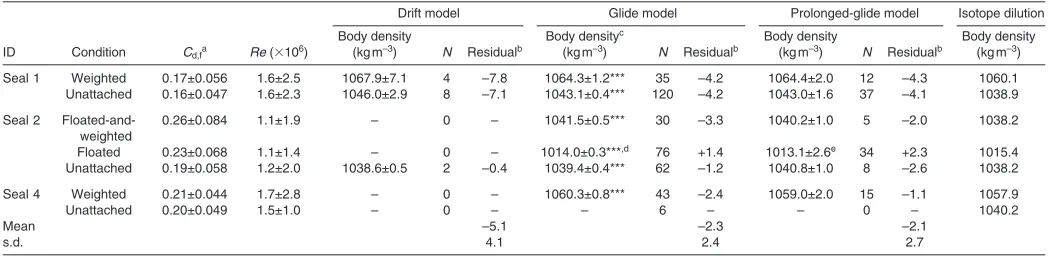
[image:6.612.44.569.90.218.2]

N4 dives and +22.5±11.6deg, N8 dives during the weighted and unattached conditions, respectively; seal 2: +27.9±2.5deg, N2 Table 2. Comparison of body density estimated from three hydrodynamic models and the body density measured using the isotope dilution

method

Drift model Glide model Prolonged-glide model Isotope dilution

Body density Body densityc _{Body density Body density}

ID Condition Cd,fa Re (⫻106) (kgm–3) N Residualb (kgm–3) N Residualb (kgm–3) N Residualb (kgm–3) Seal 1 Weighted 0.17±0.056 1.6±2.5 1067.9±7.1 4 –7.8 1064.3±1.2*** 35 –4.2 1064.4±2.0 12 –4.3 1060.1 Unattached 0.16±0.047 1.6±2.3 1046.0±2.9 8 –7.1 1043.1±0.4*** 120 –4.2 1043.0±1.6 37 –4.1 1038.9

Seal 2 Floated-and- 0.26±0.084 1.1±1.9 – 0 – 1041.5±0.5*** 30 –3.3 1040.2±1.0 5 –2.0 1038.2

weighted

Floated 0.23±0.068 1.1±1.4 – 0 – 1014.0±0.3***,d _{76 +1.4 1013.1±2.6}e _{34 +2.3 1015.4}

Unattached 0.19±0.058 1.2±2.0 1038.6±0.5 2 –0.4 1039.4±0.4*** 62 –1.2 1040.8±1.0 8 –2.6 1038.2

Seal 4 Weighted 0.21±0.044 1.7±2.8 – 0 – 1060.3±0.8*** 43 –2.4 1059.0±2.0 15 –1.1 1057.9

Unattached 0.20±0.049 1.5±1.0 – 0 – – 6 – – 0 – 1040.2

Mean –5.1 –2.3 –2.1

s.d. 4.1 2.4 2.7

a_{Drag coefficient with Re was calculated from horizontal gliding.}

b_{The difference calculated by subtracting the body density of the models from that of isotope dilution method.} c_{Estimated values ± s.e. are shown. ***, P<0.001.}

dives). The start and end depths of the drift segment (i.e. U2phase)

were 246±19 and 423±39m for the weighted condition in seal 1 (N4 dives), 213±63 and 319±33m for the unattached condition in seal 1 (N8 dives), and 298±35 and 368±24m for the unattached condition in seal 2 (N2 dives), respectively. The mean duration of drift segments was 428±161s (N14 dives).

Drag coefficient for prolonged-glide and glide models For the glide and prolonged-glide models, we used the value of Cd,f

obtained during each attachment condition for each seal to estimate the body density of the animals (Table2). There were no significant differences in Cd,fbetween the weighted and unattached conditions

for seals 1 and 4 (Mann–Whitney U-test, seal 1, U501015, P0.19;

seal 4,U501033, P0.23). However, Cd,fwas significantly different

among the three different conditions for seal 2 (Kruskal–Wallis test, 2

224.6, P<0.001). Seal 2 was the seal to which the float remained

attached, and the results suggest that attachment of the float increased the drag coefficient despite the streamlined plastic housing that provided a consistent alteration in frontal area with or without the float.

Calculation of body density: glide method

From the three seals combined, we recorded a total of 372 ascending and descending glides that met the analytical criteria. Insufficient glide data were obtained from the unattached condition for seal 4. The glides had an absolute value of pitch of 47.3±11.9deg (N372 glides). Acceleration ranged from –0.093 to 0.083ms–2 _{and was}

affected by the animal’s speed prior to initiating the glide and its pitch during the glide. The overall range of speed was 0.63 to 1.80ms–1_{and varied depending on attachment conditions for each}

seal (1.19–1.80 and 0.71–1.54ms–1_{for the weighted and unattached}

conditions in seal 1, respectively; 0.69–1.12, 0.63–1.22 and 0.74–1.30m s–1_{for the floated-and-weighted, floated and unattached}

conditions in seal 2, respectively; 1.10–1.61 and 1.06–1.24m s–1

for the weighted and unattached conditions in seal 4, respectively). The mean duration of glides, excluding prolonged glides of more than 1min, was 17.5±11.1s (N46 glides, min. 8s). Theoretical acceleration from the model corresponded well with observed acceleration when an appropriate value of the body density, obtained by least-squares methods, was used (see Fig.2 for one example). Model fits of estimated body density were all statistically significant at P<0.001 for all conditions of all seals (Table2). The absolute value of the mean difference between observed acceleration and predicted acceleration values was 0.0177ms–2_.

Calculation of body density: prolonged-glide method A total of 111 prolonged glides during ascent and descent meeting the analytic criteria were obtained from the three seals (Table2). No prolonged glides were observed in the unattached condition in seal 4. Mean absolute pitch of dives used for this analysis was 45.3±7.9deg (N111 prolonged glides). After the start of prolonged glides, measured speed gradually decreased and then remained relatively constant thereafter (see Results, Changes in stroking patterns from body density manipulations). When appropriate values of body density obtained by least squares were used, the theoretical speeds corresponded well with the observed speeds (see fig.6 in Watanabe et al., 2006).

Comparison among three hydrodynamic models

The body densities estimated from all three hydrodynamic models were highly correlated with each other (drift model vs prolonged-glide model, r2_{0.949; prolonged-glide model vs glide model,}

r2_{0.996; glide model vsdrift model, r}2_{0.977). The body densities}

estimated from the prolonged-glide model were close to the body densities estimated from the glide model (within ±1.5kgm–3_;

Table2). The differences between the body densities estimated from the drift model and the other two model approaches were somewhat greater; the range of the differences from the glide model and the prolonged-glide model was –0.8–3.6 and –2.2–3.5kgm–3_,

respectively (Table2).

Comparison of body density measured using isotope dilution Body density calculated with the isotope dilution method was similar among the three seals (range1038.2–1040.2kgm–3_{; unattached}

condition in Table2). We combined the body density estimated from isotope dilution in the unattached condition with the effect of the weights and floats to estimate the density of each seal in each attachment condition (Table2, final column). The estimated densities in the different attachment conditions were highly correlated with body densities estimated from the drift model (F1,120.5, P<0.001, r2_{0.954), the glide model (F}

1,4603.3, P<0.001, r20.992) and the

prolonged-glide model (F1,4399.9, P<0.001, r20.988; Fig.3). In

most cases, densities estimated with the hydrodynamic models were slightly higher than those estimated using isotope dilution methods (Table2).

Changes in stroking patterns from body density manipulations

Examples of stroke patterns of all conditions for each seal are shown in Fig.4. The three primary stroking patterns were observed: prolonged glide, stroke-and-glide and continuous stroking (Sato et al., 2003; Miller et al., 2004; Watanabe et al., 2006). Prolonged glides were marked by extended periods with no active strokes, and a gradual change in swim speed (Fig.4A–C,E,F). Stroke-and-glide

0.20

0.15

0.10

0.05

0

–0.05

–0.10

–0.15

Acceler

a

tion (m

s

–2

)

1.2 1.1 1.0 0.9 0.8 0.7 0.6

Swim speed (m s–1₎

–50 0

Pitch (deg) Measured acceleration

Theoretical acceleration, 1041.5 kg m–3 Theoretical acceleration, 1060.0 kg m–3

was characterized by intermittent strokes with corresponding oscillations of swim speed (Fig.4D,E,G). Continuous stroking showed relatively constant speed (Fig.4A–C,F,G).

Weighted vsunattached conditions in seals 1 and 4 Stroking patterns were similar in both conditions in seal 1, but different between conditions in seal 4. Seal 1 employed prolonged glides during descent (weighted, N18 dives, 90.0% of dives; unattached, N54 dives, 80.6%) and continuous stroking during ascent in both conditions (weighted, N20 dives, 100%; unattached,

N61 dives, 97.0%; Fig.4A,B). Similarly, seal 4 employed prolonged glides during descent (N22 dives, 100%) and continuous stroking during ascent (N22 dives, 100%; Fig.4C) in the weighted condition. In contrast, seal 4 employed stroke-and-glide at both descent and ascent in the unattached condition (descent, N34 dives, 94.4%; ascent, N33 dives, 91.7%; Fig.4D). In both seals, the descent stroke rate was lower in the weighted condition than the unattached condition, whereas the ascent stroke rate was higher in the weighted condition than in the unattached condition (Table3). During ascent, the amplitude of the lateral acceleration was significantly greater in the weighted condition than in the unattached condition in both seals (Table3).

Floated vsunattached and floated-and-weighted conditions in seal 2

The stroke pattern in the floated condition was clearly different from the other two conditions. During descent, seal 2 employed prolonged glides (N33 dives, 63.4%) for the floated-and-weighted condition, continuous stroking (N45 dives, 100%) for the floated condition and, continuous stroking (N25 dives, 36.2%) or stroke-and-glide (N24 dives, 34.8%) for the unattached condition (Fig.4E–G). During ascent, this seal displayed stroke-and-glide (N41 dives, 78.8%) for the floated-and-weighted condition, prolonged glides

(N40 dives, 88.9%) for the floated condition and continuous stroking (N69 dives, 100%) for the unattached conditions (Fig.4E–G). During descent, this seal showed a higher stroke rate in the floated condition than in either of the other two conditions, whereas during ascent, a lower stroke rate was observed in the floated condition than in either of the other two conditions (Table3). The fastest swim speeds were measured in the unattached condition in both descent and ascent (Table3). The seal exhibited relatively large amplitude of lateral acceleration when it swam against the direction of buoyancy in all three conditions (Table3).

Adjustment of stroke cycle frequency and amplitude of lateral acceleration in response to changing propulsive force These analyses were conducted for the weighted and unattached conditions in seals 1 and 4 and the unattached condition in seal 2 because the presence of the float (i.e. floated-and-weighted and floated conditions) altered the drag coefficient and appears to have affected the speed at which seal 2 swam. The optimal speed of swimming animals is expected to be proportional to (basal metabolic rate/drag)1/3_{(Alexander, 1999; Sato et al., 2010). It is reported that}

swim speed decreased when drag was experimentally increased in African penguins (Wilson et al., 1986). Thus, the increase of the drag coefficient may have led to the decrease in swim speed for the floated-and-weighted and floated conditions in seal 2. These conditions for seal 2 were not included for this analysis because the drag coefficient and swim speed, which strongly affect the resistance force, were outliers.

The amplitude of lateral acceleration and stroke cycle frequency in relation to the resistance force is shown in Fig.5. We investigated whether the changes in lateral acceleration amplitude and stroke cycle frequency with resistive force varied between individuals. This statistical model regressed the resistance force as the dependent variable against the amplitude of lateral acceleration, stroke cycle frequency and seal ID as fixed independent factors, and the interaction among these three factors was assessed with F-statistics (Fox, 2002). The three-way interaction was significant (F2,25837.33, P<0.001), indicating that the pattern in which the amplitude of lateral acceleration and stroke cycle frequency varied against resistance force differed between individuals. We therefore regressed resistive force on stroke cycle frequency, the amplitude of lateral acceleration and their interaction separately for each individual (Table4). The adjusted r2_{of the multiple regression models was high, indicating}

that much of the variation in force overcome is captured by the two measured variables (seal 1, r2_{0.887, F}

3,10472738, P<0.0001; seal

2, r2_{0.651, F}

3,1057666.1, P<0.0001; seal 4, r20.885, F3,4751230, P<0.0001).

The amplitude of lateral accelerations positively correlated with the resistance force for all seals (see Slope of independent variables in Table4). The partial correlation coefficient of the amplitude of lateral accelerations was higher than that for stroke cycle frequency for all seals (Table4). Stroke cycle frequency was positively correlated with resistive force in seals 1 and 2, but not in seal 4 (Table4). There was a significant interaction term for seal 1, suggesting that changes in stroke cycle frequency and amplitude of lateral accelerations were not made independently by that seal. Running the same analysis using active-to-passive drag ratios of 0.5 and 2.0 did not substantially change how amplitude of lateral acceleration and stroke cycle frequency related to resistive force.

DISCUSSION

By manipulating the body density and mass of seals, we were able to demonstrate that body density can be estimated from changes in 1080

1060

1040

1020

E

s

tim

a

ted

b

ody den

s

ity (kg m

–

3)

1080 1060

1040 1020

Measured body density (kg m–3₎

Drift model Glide model Prolonged-glide model

hydrodynamic gliding performance of free-diving animals. The presented methods should provide an approach for measuring and tracking changes in body condition of a wide spectrum of diving species. Because use of the hydrodynamic methods to measure body density does not require capturing animals to make measurements, it may be useful to study body condition of obligate marine divers,

such as cetaceans, which are difficult to capture to measure body condition using traditional methods. We also described how the seals modulated their stroking and gliding patterns with changes in buoyancy. The body densities achieved by attaching a lead weight and float ranged from 1015.4 to 1060.1kgm–3 _(Table2).

Estimated actual body lipid contents corresponding to these body 400

200 0

Depth (m)

18:10 18:15 18:20 18:25

2.5 2.0 1.5 1.0 0.5 –4 –20 2 4 –500 50 Pitch (deg) 300 200 100 0 Weighted condition in seal 1

A

S peed (m s –1 ) L a ter a l a cceler a tion (m s –2 )

Depth (m) 300

200 100 0

Depth (m)

15:24 15:28 15:32 15:36

2.0 1.5 1.0 0.5 –4 –20 2 4 0 50 Pitch (deg)

Weighted condition in seal 4

C

S peed (m s –1 ) L a ter a l a cceler a tion (m s –2 ) –50 400 200 0 Depth (m)

11:05 11:10 11:15 11:20

2.5 2.0 1.5 1.0 0.5 –4 –20 2 4 –50 0 50 Pitch (deg)

Unattached condition in seal 1

B

S peed (m s –1 ) L a ter a l a cceler a tion (m s –2 )

00:08 00:12 00:16 00:20

2.0 1.5 1.0 0.5 –4 –20 2 4 –50 0 50 Pitch (deg)

Unattached condition in seal 4

D

S peed (m s –1 ) L a ter a l a cceler a tion (m s –2) 15:00 15:05 Time (hh:mm) 15:10 2.0 1.5 1.0 0.5 –4 –20 2 4 –50 0 50 Pitch (deg)

Floated condition in seal 2

_F

S peed (m s –1 ) L a ter a l a cceler a tion (m s –2) 400 200 0 Depth (m) 2.0 1.5 1.0 0.5 –4 –20 2 4 –50 0 50 Pitch (deg)

Floated-and-weighted condition in seal 2

E

S peed (m s –1 ) L a ter a l a cceler a tion (m s –2) 400 200 0 Depth (m)

18:30 18:35 18:40 18:45

2.0 1.5 1.0 0.5 –4 –20 2 4 –500 50 Pitch (deg)

G

S peed (m s –1 ) L a ter a l a cceler a tion (m s –2 ) 400 200 0 Depth (m)

16:16 16:20 16:24 16:28

Unattached condition in seal 2

Time (hh:mm)

densities are 25.4–46.4%, as determined by modifying Eqn 5 to seallPl+lipid-free(1–Pl), where lipid-free is calculated from

pPp+aPa+bwPbw(1114.6kgm–3). This range compares well with

observed individual variations in lipid content estimated using labeled water (23.1–46.2%) (Biuw et al., 2003), and the dramatic seasonal changes in body lipid content that pinnipeds regularly undergo that often range from <20 to >40% (Crocker, 1995; Fedak et al., 1996; Beck et al., 2000). We discuss our results from both a biomechanical and an ecological perspective.

Validation of at-sea metrics of body density Hydrodynamic performance vsisotope dilution

The body density estimated from the three hydrodynamic models was highly correlated with that measured using the isotope dilution method, but the densities measured using our models were slightly greater than those estimated from body composition derived from isotope dilution estimates of total body water (Table2). It is difficult to assess which value is actually more accurate as all of these techniques are indirect measures of body composition and require certain assumptions (Reilly and Fedak, 1990; Arnould et al., 1996; Bowen and Iverson, 1998). However, the variation among the three hydrodynamic models is within 1% of the body density measurements, which means that the variation is within 2% of lipid contents (calculated from modified Eqn 5). Lipid content estimates from isotope dilution could easily vary by 3% lipid (Lukaski, 1987). Given these uncertainties and estimates of

precision, none of the measures were significantly different, and all the hydrodynamic methods provided estimates of body composition of the same order of accuracy as estimates obtained using isotope dilution. It would be useful to have an independent and direct estimate of body density in tested seals, which could theoretically be accomplished using whole-body air-displacement plethysmography (Fields et al., 2005).

Although differences between the estimated body densities using the isotope dilution method and the hydrodynamic models were quite small, it is worth mentioning possible errors in our hydrodynamic body-density analyses. All methods require an estimate of the drag force acting on the body. Biuw et al. pointed out that the drag coefficient is the most important factor in predicted body density for the drift model (Biuw et al., 2003). As they suggested (Biuw et al., 2003), we should not expect the drag coefficient to be constant. The drag coefficient of a diver may be affected by changes in the animal’s shape (e.g. girth, fineness ratio) due to gains or losses of lipid. The single value of the drag coefficient used in the drift method might be improved upon by considering how changes in body form might influence the drag coefficient (Vogel, 1994). Additionally, because elephant seals passively descended like a ‘falling leaf’ during drift dives (Mitani et al., 2009), postural changes against the direction of drift will result in variations in the drag coefficient. Mitani et al. reported that the pitch of animals was close to horizontal (see data supplement in Mitani et al., 2009), whereas our animals showed Table3. Comparison of stroking patterns and swim speed among experimental body-density manipulation conditions for each seal

No. Dive Amplitude of lateral

of depth Pitch (deg) Stroke rate

a_(s–1_{) Swim speed}b_(ms–1_{) acceleration}b,c_(ms–2₎

ID Condition dives (m) Descent Ascent Descent Ascent Descent Ascent Descent Ascent

Seal 1 Weighted 20 358±80 –42.2±7.7 47.7±7.9

*** 0.10±0.17 ***—– 1.93±0.13 *** 1.51±0.13 *** 1.50±0.12 NS 1.85±0.73 ***—– 3.98±0.30 _*** Unattached 67 301±91 –44.7±7.7 37.1±7.4

再

0.24±0.29 ***—– 1.68±0.19

冎

1.22±0.18

冎

1.54±0.16

冎

1.56±0.17 ***—– 2.36±0.20

冎

Seal 2 Floated-and- 52 191±110 –32.5±5.6 37.8±4.7 0.22±0.13 ***—– 1.31±0.16 0.76±0.06 0.83±0.09 0.71±0.17 ***—– 1.17±0.34

weighted

Floated 45 281±102 –48.9±6.2 45.6±6.3 *** 1.91±0.09 ***—– 0.11±0.20 *** 0.99±0.11 *** 0.91±0.09 *** 1.49±0.25 ***—– 0.80±0.23 *** Unattached 69 242±94 –36.0±7.4 36.2±8.3

冦

1.20±0.45 ***—– 1.78±0.17

冧

1.07±0.13

冧

1.12±0.13

冧

1.25±0.22 ***—– 2.57±0.35

冧

Seal 4 Weighted 22 276±67 –42.7±3.8 36.7±6.1

*** 0.15±0.05 ***—– 1.53±0.07 *** 1.33±0.07 *** 1.29±0.08 *** 1.39±0.15 ***—– 3.45±0.26 *** Unattached 36 172±42 –34.5±5.6 30.3±3.9

再

1.16±0.10_{—– 1.13±0.15}NS

冎

_1.12±0.05

冎

_1.13±0.13

冎

_{1.38±0.10 ***—– 2.20±0.19}

冎

a_{Stroke rate was compared among experimental body-density manipulation conditions and between descent and ascent using GLM with Poisson error distribution.}

b_{Swim speed and amplitude of lateral acceleration were compared among experimental body-density manipulation conditions using t-test for seals 1 and 4 and one-way ANOVA for} seal 2.

c_{Amplitude of lateral acceleration was compared between descent and ascent using t-test.} ***, P<0.001; NS, not significant.

Table4. Multiple regression models describing the effect of stroke cycle frequency and the amplitude of lateral acceleration and their interaction on resistance force

Seal 1 Seal 2 Seal 4

t P t P t P

Slope of independent variables

Stroke cycle frequency 88.2 15.32 <0.0001 19.6 2.37 <0.05 1.8 0.12 0.905

Amplitude of lateral acceleration 26.0 13.06 <0.0001 9.5 2.78 <0.01 12.1 2.04 <0.05

Stroke cycle frequency _⫻Amplitude of lateral acceleration –11.7 –5.94 <0.0001 1.8 0.50 0.619 11.5 1.59 0.113

Intercept –71.5 5.27 <0.0001 –21.0 –2.79 <0.01 –13.8 –1.11 0.268

Adjusted R2_{for the full model 0.887 0.651 0.885}

Partial r2

Resistance force vs Stroke cycle frequency 0.506 0.212 0.159

Resistance force vs Amplitude of lateral acceleration 0.791 0.783 0.929

a slightly greater degree of head-up orientation during drift dives. We did not assess the estimated body density in relation to postural changes because we only recorded 14 drift dives, but the relatively large variation in body density estimated from the drift model may arise from changes in the drag coefficient during drift dives that are caused by postural differences.

For both the prolonged-glide and glide models, the drag coefficients used in the body density model were measured from horizontal glides (Bilo and Nachtigall, 1980). We expect that induced drag generated by lift-producing organs that help the animal maintain a non-vertical posture and direction of movement should influence the forces acting on the animal during non-vertical glides. If so, our estimate of the drag coefficient from horizontal glides, ignoring the effects of induced drag, may be an overestimate of body drag. At the same time, induced drag is expected to be generated during any glides or prolonged glides that are not perfectly vertical. In fact, the glides and prolonged glides we used to estimate body density had a mean pitch of 47.3±11.9 and 45.3±7.9deg, respectively.

Estimated body density matched very closely density estimates from the isotope dilution method, ignoring the effects of lift-induced drag (Table2). That result suggests that the magnitude of induced drag during horizontal and more vertical glides was small and/or that the effect of ignoring induced drag during horizontal glides is partly cancelled by also ignoring induced drag during the steeper ‘vertical’ glides, which in fact deviated from a perfectly vertical orientation. However, in the one case where we were able to make an estimate of induced drag, the floated condition in seal 2, the estimated corrected drag coefficient was 65–78% of the drag coefficient calculated from horizontal glides (see Appendix), indicating that our calculation using horizontal glides was an overestimation of the drag coefficient. But, using the adjusted drag coefficient did not make much difference to the agreement with the body density estimated from isotope dilution method (glide model, pre-adjustment +1.4kgm–3_{, adjustment –2.1kgm}–3_;

prolonged-glide model, pre-adjustment +2.3kgm–3_{, adjustment –1.6kgm}–3_;

residual in Table2). Further research describing the lift-producing mechanisms in diving seals is required to better predict levels of 60

50

40

30

20

10

0

–10

6 5 4 3 2 1 0

Amplitude of lateral acceleration (m s–2₎

1.4 1.3 1.2 1.1 1.0 0.9 0.8 0.7 0.6 0.5

Stroke cycle frequency (Hz) Seal 2

80

60

40

20

0

F

orce (N)

Seal 4 100

80

60

40

20

0

–20

Seal 1

Weighted : Ascent Descent

induced drag, which could improve body density estimation in free-swimming animals.

Advantages and disadvantages of the different hydrodynamic models

The analyzing criteria, necessary variables and required behaviours needed for the three methods to estimate body density using hydrodynamic performance models are presented in Table5. The simplest method is the drift model, because this model requires only dive time vsdepth profiles as recorded by data logging and telemetry instruments. However, to our knowledge, only a few species including elephant seals exhibit drift dives [e.g. New Zealand sea lions (Crocker et al., 2001a), sperm whales (Miller et al., 2008) and New Zealand fur seals (Page et al., 2005)], which limits its applicability to many species. In contrast, common stroking patterns (i.e. prolonged-glide and stroke-and-glide) have been observed across a wide taxonomic range, including cetaceans, pinnipeds, sea turtles and sea birds (e.g. Williams et al., 2000; Sato et al., 2003; Miller et al., 2004; Watanuki et al., 2005; Watanabe et al., 2006; Hays et al., 2007). Therefore, the methods using prolonged-glide and glide models are potentially applicable to a wider range of species compared with methods using the drift-dive model.

The prolonged-glide model requires that terminal speed be represented by a constant speed. We predicted the time required to reach terminal speed using measured body densities. The time to reach theoretical terminal speed increases as the density difference between the animal and the surrounding water decreases, so terminal speed can be more readily measured when body density differs from that of seawater. Although aquatic animals usually swim at 1–2ms–1

during descent and ascent (e.g. Sato et al., 2007), the theoretical terminal speed of neutrally buoyant animals is zero, essentially making terminal speed unavailable as an estimator. However, animals rarely remain in a state of neutral buoyancy for long (Biuw et al., 2007; Robinson et al., 2010), as even small changes in body density would lead to substantial changes in the forces acting on the animal.

The glide model can be applied irrespective of the body density of the animals if stable glides of several seconds duration are recorded. The model assumes that only the combined forces of drag and buoyancy cause deceleration or acceleration during glides. However, rapid maneuvers of the animals or manipulations of body drag by the animal would violate that assumption. Although we might expect that animals will typically glide in an efficient manner to reduce locomotion costs, it is important to inspect body posture

during glides to exclude unstable glides. In addition, the glide model requires accurate and frequent measures of swim speed because acceleration and deceleration during glides are based on relatively short-term changes in swim speeds.

Changes in stroking patterns resulting from body density manipulations

Our experiment clearly showed that changes in body density affected stroke rate and the proportion of time gliding. We simulated a reduction of body lipid by increasing the body density by attaching a lead weight to seals 1 and 4. The increased density caused the descent stroke rate to decrease and the ascent stroke rate to increase. Watanabe et al. reported similar results: descent stroke rate was lower during the weighted condition compared with the unattached condition whereas ascent stroke rate was higher in the weighted condition compared with the unattached condition (Watanabe et al., 2006). We also simulated increased fat content by attaching a float. When the lead weight was detached from the seal that was initially in the floated-and-weighted condition (seal 2), its descent stroke rate increased and the ascent stroke rate decreased.

The amplitude of lateral acceleration positively correlated with the resistance force caused by drag and buoyancy, suggesting that our animals adjusted the stroke intensity in response to changes in resistant force. In general, muscle fibers have their highest power output and efficiency over a relatively narrow range of contraction speeds and loads (Hill, 1950; Hill, 1964; Lovvorn et al., 1999). Therefore, it is possible that swim speed could be altered to bring about compensatory changes in thrust force against drag and buoyancy, thereby conserving thrust stroke force (supplementary material Fig.S2). For example, in case of seal 1, mean speed at ascent was 1.50ms–1_{, which required an 87N}

propulsive force (see Materials and methods, Stroking patterns for the calculation; supplementary material Fig.S2). If the seal conserved the thrust force (i.e. 87N) irrespective of buoyancy, swim speed in the unattached state would have become faster because release of the lead weight dramatically lowered buoyancy resistance (expected speed, 2.1m s–2_{; supplementary material}

Fig.S2). During descent, swim speed at both conditions would also become faster because buoyancy aids the seal’s swimming (expected speed, 2.6ms–1 _{for unattached and 3.0ms}–1 _for

weighted; supplementary material Fig.S2). However, the seals usually swam at 1–1.5ms–1_{during active stroking in all conditions}

[image:12.612.43.572.79.178.2]

(Fig.4). We suggest that the seals adjusted propulsive force to maintain swim speed within a narrow range, despite changes in Table 5. Required logging parameters and conditions for three hydrodynamic models

Models Logging parametersa,b _Conditiona

Drift model Depth (>100 m) Drift dives

Prolonged-glide model Depth (>100 m) Prolonged-glides (reaching terminal speed)

Accelerationc _{(兩Pitch兩>30 deg)} Swim speed

Glide modeld _{Depth (>100 m) (Stable) glides}

Accelerationc_{(兩Pitch兩>30 deg)} Swim speed

a_{Parentheses show criteria for analysis in this study.}

b_{Seawater density is not a necessary logging parameter but better provides an estimation of body density in all models if it is recorded.}

c_{Pitch is calculated from longitudinal acceleration (see Materials and methods). To extract ‘prolonged-glides or glides’, acceleration of the axis which is}