Variable Daily Air Temperature Model for Analysis and Design

(1)

ISSN Print: 2152-7385

DOI: 10.4236/am.2018.98069 Aug. 30, 2018 1015 Applied Mathematics

Variable Daily Air Temperature Model for

Analysis and Design

G. Danko

1,2

, C. Lu

1

1_{Mackay School of Earth Science and Engineering, University of Nevada, Reno, Reno, NV, USA} 2_{Research Institute of Applied Earth Sciences, University of Miskolc, Miskolc, Hungary}

Abstract

An analytical model, T tA

( )

, for the observed outside air temperature change,

( )

a

T t , with time is developed using two components: one for the variation caused by the Earth’s movement, plus any other quasi-stationary thermody-namic effects due to industrialization; and one for the random variation caused by stochastic and/or chaotic, local environmental changes. The first component, T tR

( )

, describes a regular trend, expressed by periodic functions

of time and constants unchanged with time. The second component, TS, is a

random, stochastic variation. For the observed outside air temperature, the analytical model of T tA

( )

=T t TR

( )

+ S is such as to give a statistically best

approximation for the observed time period with T t T ta

( )

− A

( )

=min. Sev-eral versions for the T tR

( )

functions are defined and tested in the study for

an example location for 20 years. The best model for T tR

( )

is found as a

li-near function with time plus a variable-coefficient Fourier series with lili-nearly changing amplitude with time. It is found that the final analytical tempera-ture, T tA

( )

, can be used not only to represent the historical daily mean

tem-perature but also to predict the future daily mean temtem-perature at the given location. The upper and lower boundaries give safety limits for the tempera-ture prediction. The stochastic component identified in the model is stable and stationary. The method of model identification for T tA

( )

can be used

for determining input temperature functions for supporting engineering de-sign; or for an unbiased scientific inquiry of temperature change with time in climate studies.

Keywords

Air Temperature Model, Deterministic and Stochastic Changes, Temperature Trends

How to cite this paper: Danko, G. and Lu, C. (2018) Variable Daily Air Temperature Model for Analysis and Design. Applied Mathematics, 9, 1015-1038.

https://doi.org/10.4236/am.2018.98069

Received: July 3, 2018 Accepted: August 27, 2018 Published: August 30, 2018

(2)

DOI: 10.4236/am.2018.98069 1016 Applied Mathematics

1. Introduction

Climate is one of the main elements of the natural environment. Temperature has a direct impact on atmospheric stability, evaporation, precipitation, and many other conditions of life [1]. Temperature change affects living conditions, agriculture, industry, tourism and engineering designs. Atmospheric tempera-ture is needed for planning and forecasting both in the average and the variation components of temperature in order to prevent hazards to life as well as finances [2].

Based on the long-term trends study of maximum, minimum and mean an-nual air temperature, e.g., in the northwest Himalayan region during the twen-tieth century, increasing trends are seen both in the mean and the diurnal range of temperature. The daily maximum temperatures have increased more rapidly than the decrease in the low temperatures in the last century resulting in a risen mean temperature of about 1.6˚C [3]. An extrapolation for the next century would give an increase about 3˚C to 5˚C in the global mean annual temperature [4]. A more exact forward prediction approach may give different result. It is difficult, however, to analyze slowly-changing trends in the outside temperature as they are buried within large-amplitude, harmonic, cyclic variations as well as stochastic and/or chaotic changes.

The observed, outside air temperature, T ta

( )

,τ , includes both seasonal

components represented by t (days of the year) and

τ

(the hours in day t). When tabulated, T ta

( )

,τ is a matrix with t rows (the total number of days) and

τ

columns (24, the number of hours in a day). The outside air temperature has a regular, seasonal variation for the daily average temperature during every year, (more exactly, every four years as a true time period) and an hourly variation during any given day for the hourly mean temperature. These two components are regular and periodic in nature caused by the earth movement in the solar system. Other regular changes superimposed to that of the known movement of the Earth may also be present, such as caused by the heat balance of the globe by industrialization.

The goal of the paper is to separate the observed outside air temperature into variation caused by the Earth’s movement, plus any other quasi-stationary thermodynamic effects, and random variation caused by stochastic and/or chao-tic, local environmental changes. It’s necessary to separate the hourly temperate variations from that of the seasonal first. For describing the seasonal tempera-ture variation, the daily average temperatempera-ture T ta

( )

must be defined. The

( )

a

T t may be defined as the integral mean value:

( )

1 ₀T

( )

, d

a a

T t T t

T τ τ

=

_∫

₍₁₎

(3)

DOI: 10.4236/am.2018.98069 1017 Applied Mathematics pre-calculated from the Standard Model that provides the average of the daily maximum and minimum air temperatures, T ta

( )

≅Tmax

( )

t T+ min

( )

t  2. The Standard Model, reviewed by Bilbao et al.[5], may not be accurate if the tem-perature change is not symmetrical between day and night [6]. Nevertheless, the convenience in using the Standard Model instead of using the hourly tempera-ture data for every day and using the expression (1) may overwhelm the con-cerns in the accuracy of the mean, daily temperature.

Two components of the air temperature are distinguished in the present paper for modeling daily mean air temperature variation, T ta

( )

, with time. The first

component, T tR

( )

, describes a regular trend, expressed by functions of time

and constants unchanged with time over which the model is defined. The regu-lar trend is defined as stationary for a long period of time, characteristic to a given physical location governed by deterministic causes such as the Earth’s movement in the solar system. The second component, TS, is a random,

sto-chastic variation around the regular trend. The TS component is caused by the

stochastic and/or chaotic process in the atmosphere, defined as difference be-tween the observed outside air temperature, T ta

( )

, and the temperature from

the stationary trend model as TS=T Ta− R. The daily mean value of the outside

temperature at any given day is the sum of the regular trend component, TR,

and a stochastic variation part, TS:

( )

a R S

T t =T t T+ ₍₂₎

Note that the stochastic component is stationary and irrespective of the sea-sonal variation, a simplification for model formulation. However, the stochastic temperature variation in some part of the year may be more disturbed than in another, raising the possibility for improvement of the assumption used in the current work, a task left for the interested reader.

The analytic function for T tR

( )

must be the best fit to the measured outside

temperature data for a given location. The concept of Fourier’s series approxi-mation [7] is employed for constructing a model for a mainly periodic ambient air temperature, TR. Joseph Fourier, a French mathematician and physicist

in-troduced in 1807 the approximation of any function f x

( )

over a finite interval with an infinite sum of sine and cosine functions as

( )

0 i1 isin

( )

icos

( )

g x a ∞ a ix b ix

=

= +

∑

_ + _ such that f x

( ) ( )

−g x 2=min_{, where}

0, ,i i

a a b are unknown constants. An equivalent formulation may be used as

( )

0 i1 isin

(

i

)

g x =a +

∑

∞₌a ix b+ for brevity. Instead of an infinite series, i∈

[ ]

0,n is used for the approximation of a mainly periodic function, eliminating the terms multiplied by the insignificant amplitudes a i ni, > .

Applying the concept for TR with a mean temperature, Tm, and a harmonic

variation component,

∑

Aω_isin

(

ω

it+

α

i

)

, where Aω_i is the amplitude of the

harmonic variation component of f ti

( )

=sin

(

ωit+αi

)

. The amplitude, Aωi,

may be a linear function of time in some models, A tωi

( )

=d1,i+d t2,i .

There are various choices to model the TR component, listed as M1 through

(4)

DOI: 10.4236/am.2018.98069 1018 Applied Mathematics be used to describe the yearly mean temperature change. However, it does not have the ability to reflect any periodic temperature variation. The M2-type mod-el is the general Fourier series function. It assumes that the yearly mean temper-ature and amplitudes for the pre-selected, finite number of frequencies are con-stant. It might be accurate for a short period of time, such as one year. The problem with the M2-type model is that it cannot reflect the long-term average, the maximum and the minimum temperature changes with time as in Bhutiya-ni’s study [3]. The M3-type model is an updated function from the M2-type model. It has the variable yearly mean temperature with time. However, it still does not have the ability to reflect the maximum and minimum temperature changes with time. The M4-type model is an improved form over the M2-type model in terms of allowing the variation of maximum and minimum tempera-tures, but still using the constant yearly mean temperature. The M5-type model combines the advantages of both the M3-type and M4-type of models.

Therefore, the five different models tested are as follows: M1. Variable mean temperature

( )

R m

T t =T + ⋅c t₍₃₎

M2. Constant mean temperature and constant amplitude series:

( )

_i

( )

R m

T t =T +

∑

A f tω (4)

M3. Variable mean temperature and constant amplitude series:

( )

_i

( )

R m

T t =T t +

∑

A f tω (5)

M4. Constant mean temperature and variable amplitude series:

( )

_i

( ) ( )

R m

T t =T +

∑

A t f tω (6)

M5. Variable mean temperature and variable amplitude series:

( )

_i

( ) ( )

R m

T t =T t +

∑

A t f tω (7)

The M1-type model is used for comparison with other models for the yearly mean temperature variation evaluation. Bhutiyani [3] studied the average, maximum and minimum temperature trends for 100 years and found them all changing with time. Therefore, the M2-type model with a stationary, constant mean temperature and constant amplitudes is inferior for practical application and not used for comparisons. The M4-type model is not recommended nor studied for brevity as the M5-type model gives better result for the same effort. Therefore, for comparison purpose, only the M1, M3 and M5 model types are used in model testing.

(5)

Figure 1. Components of establishing an analytical temperature model.

2. Measured Temperature Data

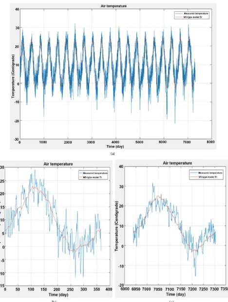
Daily mean temperature measurements are used in the study from a middle-west location in North America for 20 years. The data, T ta

( )

, are taken for 7305 days

from 04/01/1996 to 03/31/2016, downloaded from https://www.wunderground.com, and plotted in Figures 2(a). Figure 2(b) and Figure 2(c) are enlargement of Figure 2(a) for year 1 and year 20, respectively. Although the regular trend,

( )

R

T t , is to be discussed in Point 3 of the paper, it is also shown from the M5-type model in Figure 2(a). Figure 2(b) and Figure 2(c) for illustrating the model concept. The daily mean temperature data, T ta

( )

, is taken from the

Standard Model method in the study as a practical compromise. Three different ways of using the measured data are tried for comparison and to find the best way of data processing.

2.1. Single-Year Temperature Cycle Evaluation

In the first usage of the data, T ta

( )

, the measured mean daily temperatures for

20 years are divided into twenty sets for single year from 1 to 20 to be able to analyze the model validity for model type M1 and M3. Individual yearly data,

( )

, a y

T t , y∈

[

1,20

]

, t∈

[

1,365

]

are grouped for 15 regular years and t∈

[

1,366

]

for 5 leap years.

2.2. Four-Year Temperature Cycle Evaluation

In the second usage of the data,T ta

( )

, the 20 years measured mean daily

tem-peratures are divided into 4-year period sets, giving 5 groups as 1), 2), 3), 4) and 5). The justification of employing four years as the true solar time period is that the yearly time period for regular years is distorted by the deficiency of 0.25 days while the time period in leap years is longer by 0.75 days and affecting the aver-aging. The 4-year time sequence of 1461 days is considered as the repeating time period for the TS stationary temperature component in the model. Therefore,

properties of temperature (average, etc.) also must be considered distinguished when evaluating for the yearly time period.

1) For year 1 - 4:

( )

[

]

, , 1,1461 a a a

T =T t t∈ ₍₈₎

2) For year 5 - 8:

( )

[

]

, , 1462,2922 a b a

T =T t t∈ ₍₉₎

3) For year 9 - 12:

( )

[

]

, , 2923,4383 a c a

(6)

(a)

[image:6.595.66.534.65.685.2]

(b) (c)

(7)

DOI: 10.4236/am.2018.98069 1021 Applied Mathematics 4) For year 13 - 16:

( )

[

]

, , 4384,5844 a d a

T =T t t∈ ₍₁₁₎

5) For year 17 - 20:

( )

[

]

, , 5846,7305 a e a

T =T t t∈ ₍₁₂₎

2.3. Continuous, Repeating Four-Year Temperature Cycles

Evaluation

In the third usage of the data, T ta

( )

, the total 20 years 7,305 data, T ta

( )

,

[

1,7305

]

t∈ , are used for testing and establishing properties of T tR

( )

in model

type M4 and M5.

3. Determination of

TR

To determine the model coefficients, the obvious choice is to use the Least-squares (LSQ) fit method. The LSQ method optimally fits the data to a given function with unknown constant parameters in such a way that the root-mean-square of the error between model and measured data is minimalized. The expected, fitted equations represent the significant, regular temperature trend, TR. Determining the significant part of the data out of a noisy

observa-tion may also be done by filtering or neural network. The advantage of using the LSQ method is to be able to define function TR in advance, whereas signal

processing does not give an analytical form of such a function [8].

For supporting the ways of using measured data, different fitting function may be defined with a number of unknown parameters to be determined by the LSQ fitting algorithm. Five different fitting functions may be considered for M1, M3 and M5 model types as follows.

3.1. T

R

Function for the Entire 20 Years for M1-Type Model

The LSQ linear function is:

mt m

T =T + ⋅c t (13)

3.2. T

R

Function for M3-Type Model

For single year data in the M2-type model, a regular year of 365 days and a leap year of 366 days must be distinguished. The LSQ function for regular year is written as:

( )

(

)

(

)

(

)

(

)

, 1 1 1 2 2 2

3 3 3 15 15 15

sin 2π sin 2π

R y m

T t T c t A t a b A t a b

A t a b A t a b

= + × + × × × + + × × × +

+ × × × + + +_ × × × + (14)

where 1

{

{ } { }

₂ 1 _{,3 2} 1

}

365 i j

k

a ₌ _× − _× − _{; for}_k_∈

[ ]

_1,15 _, _{k i j}_{= +} _; _{i i}_{= ∈}

[ ]

_1,8 _;

[ ]

1,7

j∈ _{, all fixed frequency components. Unknown parameters are}_T_m,_c_,_A₁ through A15, and b1 through b15.

(8)

( )

(

)

(

)

(

)

(

)

, 1 1 1 2 2 2

3 3 3 15 15 15

sin 2π sin 2π

R y m

T t T c t A t a b A t a b

A t a b A t a b

= + × + × × × + + × × × +

+ × × × + + + × × × + (15)

where 1

{

{ } { }

₂ 1 _{,3 2} 1

}

365

i j

k

a ₌ _× − _× − _{; for}_k_∈

[ ]

_1,15 _, _{k i j}_{= +} _; _{i i}_{= ∈}

[ ]

_1,8 _;

[ ]

1,7

j∈ _{, all fixed frequency components. Unknown parameters are}_T_m,_c_,_A₁ through A15, and b1 through b15.

The LSQ function for 4 years data and 20 years data will add the four-year and two-year period frequencies, also will change the one-year period to 365.25 days, the function is written as:

( )

(

)

(

)

(

1

)

1 1 2

(

2

)

2

3 3 3 17 17 17

sin 2π sin 2π

R m

T t T c t A t a b A t a b

A t a b A t a b

= + × + × × × + + × × × +

+ × × × + + + × × × + (16)

where 1

{

{ } { }

₂ 3 _{,3 2} 1

}

365.25

i j

k

a ₌ _× − _× − _{; for}_k_∈

[

_1,17

]

_, _{k i j}_{= +} _; _{i i}_{= ∈}

[ ]

_1,10 _;

[ ]

1,7

j∈ _{, all fixed frequency components. Unknown parameters are}_T_m,_c_,_A₁ through A17 and b1 through b17.

3.3. T

R

Function for M5 Type Model

With the assumption that the amplitudes may also vary with time, a modified LSQ function over (16) is established as:

( )

(

)

(

)

(

)

(

)

(

)

(

)

1 1 1 1

2 2 2 2

17 17 17 17

sin 2π

R m c v

c v

T t T c t A A t t a b

A A t t a b

A A t t a b

= + × + + × × × × +

+ + × × × × + +

+ + × × × × +

 (17)

where 1

{

{ } { }

₂ 3 _{,3 2} 1

}

365.25

i j

k

a ₌ _× − _× − _{; for}_k_∈

[

_1,17

]

_, _{k i j}_{= +} _; _{i i}_{= ∈}

[ ]

_1,10 _;

[ ]

1,7

j∈ _{, all fixed frequency components. Unknown parameters are}_T_m,_c_, A₁_c through A17c, A1v through A17v, and b1 through b17.

4. Evaluation of the Statistically Most Significant, Mean

Temperature Trends

The LSQ fitting method is used to determine the mean temperature trend,

( )

R

T t , of the measured data, T ta

( )

. The LSQ method provides the statistically

most significant result for T tR

( )

as a regular, deterministic trend, depressing

the random variation component of temperature around T tR

( )

with assumed,

normal distribution as a noise due to stochastic or chaotic causes.

First, the best LSQ fit is determined on all single year data separately. The pa-rameters of function (14) are applied for the regular years, and (15) is applied for the leap years. The fitted results are shown in Figure 3(a), Figure 3(b) and Fig-ure 3(c). The mean, maximum and minimum values from the fitted result are shown in Figure 4.

(9)

(a)

[image:9.595.63.540.63.691.2]

(b) (c)

(10)

Figure 4. The mean, maximum and minimum values for LSQ fitting results for each year.

result are shown in Figure 6. Parameters for the fitted functions Ta a,

( )

t , , T ta e,

( )

,

are listed in Tables 1-5, respectively.

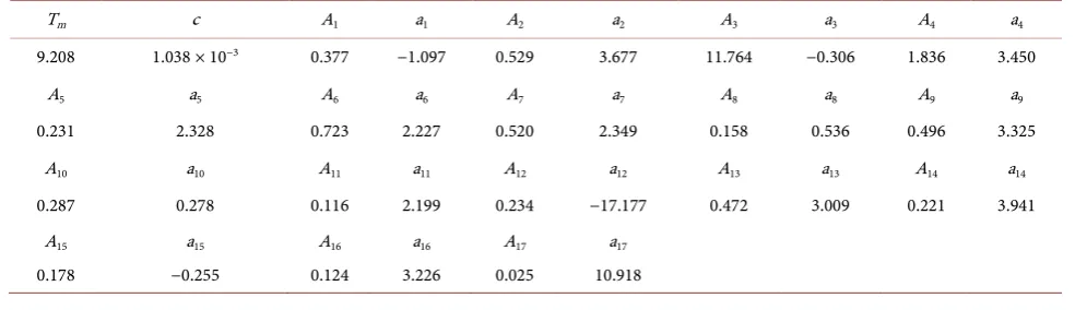
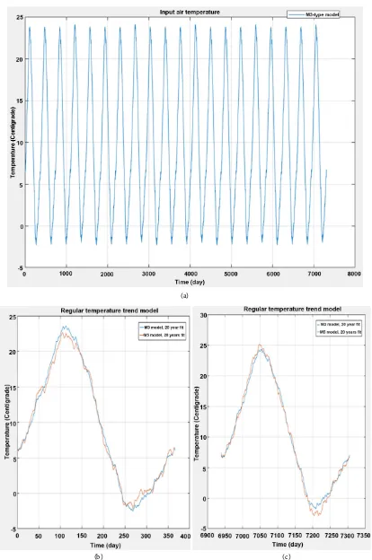
Third, the best LSQ fit is determined using the M3-type function (16) for all 20 years data, T ta

( )

, together. The fitted function is depicted in Figure 7(a),

Figure 7(b) and Figure 7(c). The parameters of the fitted function are listed in Table 6. The best LSQ fit is also determined using the improved, M5-type func-tion (17), applied also for all 20 years data, T ta

( )

. The fitted results are depicted

in Figure 8(a), Figure 8(b) and Figure 8(c); and the parameters of the fitted function are listed in Table 7.

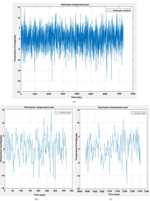
5. Evaluation of the Stochastic Variation and Final Analytical

Temperature Model

The stochastic variation must be defined by subtracting the statistic periodic function from the measured data. First, the stochastic variation, T tS

( )

, is

de-fined by the difference between deterministic function result, T tR

( )

and

meas-ured data T ta

( )

as:

( )

S a R

T t =T t T t− ₍₁₈₎ The data of (18) is depicted in Figure 9(a), Figure 9(b) and Figure 9(c). The density analysis on the (18) data and the MATLAB normal distribution fit of the data is shown in Figure 10. From the fit, a mean value _mu_{= −}_{6.33 10}_× −8_≈₀_, and standard deviation of σ =4.0012_{are obtained, where}mu=

∑

T t n_S

( )

_,

( )

(

)

2

1

S

T t mu n

σ =

∑

− _and_n_{is the number of days,}_t_{. Using} mu=0.00_and 4.0012

(11)

(a)

[image:11.595.60.531.62.688.2]

(b) (c)

(12)

[image:12.595.59.539.68.382.2]

[image:12.595.54.545.437.553.2]

Figure 6. The mean, maximum and minimum values for LSQ fitting results for 4-year sets.

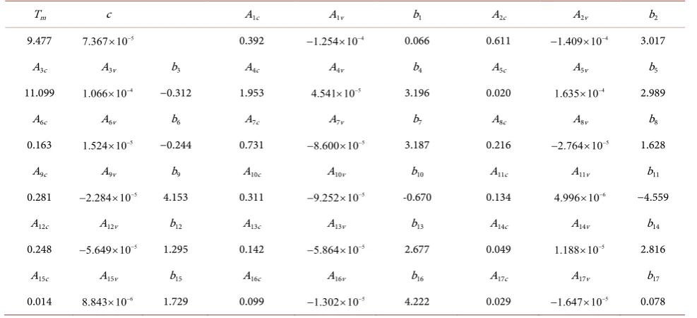
Table 1. Parameters for year 1 - 4 data, the LSQ fitted function (16) result, Ta a, .

Tm c A1 a1 A2 a2 A3 a3 A4 a4

0.731 −2.48 × 10−4 _0.527 _0.982 _0.282 _2.468 _10.616 _−0.343 _2.281 _3.248

A5 a5 A6 a6 A7 a7 A8 a8 A9 a9

0.257 2.759 0.584 −0.816 0.798 2.985 0.072 −0.525 0.399 4.295

A10 a10 A11 a11 A12 a12 A13 a13 A14 a14

0.285 −0.807 0.181 −17.310 0.154 1.797 0.117 0.950 0.092 3.044

A15 a15 A16 a16 A17 a17

0.080 1.639 0.142 4.827 0.043 1.059

Table 2. Parameters for year 5 - 8 data, the LSQ fitted function (16) result, Ta b, .

Tm c A1 a1 A2 a2 A3 a3 A4 a4

9.208 1.038 × 10−3 _0.377 _−1.097 _0.529 _3.677 _11.764 _−0.306 _1.836 _3.450

A5 a5 A6 a6 A7 a7 A8 a8 A9 a9

0.231 2.328 0.723 2.227 0.520 2.349 0.158 0.536 0.496 3.325

A10 a10 A11 a11 A12 a12 A13 a13 A14 a14

0.287 0.278 0.116 2.199 0.234 −17.177 0.472 3.009 0.221 3.941

A15 a15 A16 a16 A17 a17

[image:12.595.52.550.588.730.2]

(13)

[image:13.595.54.546.92.230.2]

Table 3. Parameters for year 9 - 12 data, the LSQ fitted function (16) result, Ta c, .

Tm c A1 a1 A2 a2 A3 a3 A4 a4

10.735 −1.715 × 10−3 _1.028 _3.156 _0.756 _2.810 _11.843 _−0.268 _1.931 _3.252

A5 a5 A6 a6 A7 a7 A8 a8 A9 a9

1.239 2.354 0.431 −0.535 0.766 −1.907 0.558 1.876 0.381 −0.040

A10 a10 A11 a11 A12 a12 A13 a13 A14 a14

0.372 1.158 0.195 3.605 0.341 −0.427 0.073 4.363 0.157 1.924

A15 a15 A16 a16 A17 a17

[image:13.595.54.543.264.391.2]

0.167 2.334 0.036 4.023 0.044 4.296

Table 4. Parameters for year 13 - 16 data, the LSQ fitted function (16) result, Ta d, .

Tm c A1 a1 A2 a2 A3 a3 A4 a4

9.242 2.539 × 10−4 _0.645 _0.197 _0.427 _−0.565 _11.355 _−0.357 _2.566 _3.116

A5 a5 A6 a6 A7 a7 A8 a8 A9 a9

0.543 3.556 0.790 0.205 0.723 3.246 0.252 2.302 0.482 3.649

A10 a10 A11 a11 A12 a12 A13 a13 A14 a14

0.417 2.377 0.592 1.153 0.175 2.700 0.153 2.907 0.084 −7.709

A15 a15 A16 a16 A17 a17

0.077 2.546 0.046 0.520 0.100 3.479

Table 5. Parameters for year 17 - 20 data, the LSQ fitted function (16) result, Ta e, .

Tm c A1 a1 A2 a2 A3 a3 A4 a4

10.289 1.073 × 10−4 _0.883 _3.050 _0.372 _0.298 _11.798 _−0.288 _2.138 _2.958

A5 a5 A6 a6 A7 a7 A8 a8 A9 a9

1.234 3.131 0.412 10.828 0.110 1.318 0.206 4.330 0.308 −0.624

A10 a10 A11 a11 A12 a12 A13 a13 A14 a14

0.081 2.438 0.126 2.924 0.125 4.272 0.147 7.643 0.243 2.356

A15 a15 A16 a16 A17 a17

0.038 1.193 0.080 3.917 0.063 2.760

Table 6. Parameters for year 1 - 20 data, the LSQ fitted function (16) result.

Tm c A1 a1 A2 a2 A3 a3 A4 a4

9.489 7.367 × 10−5 _0.095 _2.478 _0.092 _3.072 _11.489 _−0.311 _2.113 _3.194

A5 a5 A6 a6 A7 a7 A8 a8 A9 a9

0.622 2.836 0.222 −0.292 0.418 3.237 0.122 1.909 0.197 4.259

A10 a10 A11 a11 A12 a12 A13 a13 A14 a14

0.123 1.122 0.153 1.723 0.041 1.358 0.121 2.682 0.093 2.957

A15 a15 A16 a16 A17 a17

[image:13.595.53.549.426.552.2] [image:13.595.55.541.586.726.2]

(14)

[image:14.595.53.547.89.314.2]

Table 7. Parameters for year 1 - 20 data, the LSQ fitted function (17) result.

Tm c A1c A1v b1 A2c A2v b2

9.477 _{7.367 10}_× −5 _0.392 ₋_{1.254 10}_× −4 _0.066 _0.611 ₋_{1.409 10}_× −4 _3.017

A3c A3v b3 A4c A4v b4 A5c A5v b5

11.099 _{1.066 10}_× −4 _−0.312 _1.953 _{4.541 10}_× −5 _3.196 _0.020 _{1.635 10}_× −4 _2.989

0.163 _{1.524 10}_× −5 _−0.244 _0.731 ₋_{8.600 10}_× −5 _3.187 _0.216 ₋_{2.764 10}_× −5 _1.628

0.281 ₋_{2.284 10}_× −5 _4.153 _0.311 ₋_{9.252 10}_× −5 _-0.670 _0.134 _{4.996 10}_× −6 _−4.559

0.248 ₋_{5.649 10}_× −5 _1.295 _0.142 ₋_{5.864 10}_× −5 _2.677 _0.049 _{1.188 10}_× −5 _2.816

0.014 _{8.843 10}_× −6 _1.729 _0.099 ₋_{1.302 10}_× −5 _4.222 _0.029 ₋_{1.647 10}_× −5 _0.078

generates t number of random values from the normal distribution with a mean value mu, and standard deviation value

σ

_{. Applying it to} T tS

( )

, it gives:

( )

(

, ,

)

S

T t =NormRandom muσ t ₍₁₉₎

For T tA

( )

, (19) is added to (17):

( )

(

, ,

)

A R

T t =T t +NormRandom mu σ t ₍₂₀₎

However, (20) is not an analytical function since it includes an algorithm. To overcome this and understanding that the daily variation for random causes is a sample of T tS

( )

, the maximum and minimum values can be generated with a

99 per cent confidence by a fluctuating temperature with a 2-day cycle time:

( )

3

( )

1t

A R

T t =T t + σ − ₍₂₁₎

Substituting the preferred model in (17), the final analytical temperature model, T tA

( )

is:

( )

(

)

(

)

(

)

(

)

(

)

(

)

( )

1 1 1 1

2 2 2 2

17 17 17 17

sin 2π

sin 2π 3 1

A m c v

c v

t

c v

T T c t A A t t a b

A A t t a b

A A t t a b

t

σ

= + × + + × × × × +

+ + × × × × + +

+ + × × × × + + −

 (22)

Comparison between simulated temperature, T tA

( )

, from (20) and measured

data, T ta

( )

, is show in Figure 11(a), Figure 11(b) and Figure 11(c). Using an

(15)

(a)

[image:15.595.92.506.64.688.2]

(b) (c)

(16)

(a)

[image:16.595.93.509.63.693.2]

(b) (c)

(17)

(a)

[image:17.595.60.540.62.706.2]

(b) (c)

(18)

[image:18.595.209.540.57.315.2]

Figure 10. Data Equation (18) result density analysis and normal distribution fit.

6. Discussion of the Results

6.1. Discussion of the Results for the Air Temperature Variation

as a Regular Trend

For comparison purposes, the linear regression function (13) for the entire 20-year data set is applied to various, fitted model results; or original, unprocessed data. The fitted model results for the shorter time periods represent the significant part of the repeated trends whereas the noise is intentionally depressed in the LSQ norm sense. Therefore, a linear regression evaluation for the 20-year long time period is assumed to evaluate the most significant, time-average of the linear change in the magnitude of T ta

( )

. Common expectation dictates that the linear

regression evaluation for the 20-year long time period of the original data may provide an un-biased result for the linear change in the magnitude of T ta

( )

.

The following studied are completed for fitting a longer-time linear regression to model results, T tR

( )

, of shorter time periods:

a) Yearly mean temperatures, T tR

( )

, (for 15 regular and 5 leap years)

eva-luated from fitted function to single-years data, Ta y,

( )

t with M1-type model;

b) Yearly mean temperatures, T tR

( )

, evaluated from fitted function data to

4-year data sets, Ta a,

( )

t , , Ta e,

( )

t with M1-type model;

c) Yearly mean temperatures, T tR

( )

, from fitted function to continuous 20

years data, T ta

( )

with M1-type model;

d) 20 years measured data, T ta

( )

, used unprocessed.

The results from the evaluation are listed in Table 8. As shown, the linear trends for the mean value, Tm, and the slope, c, are very similar for cases a) and

(19)

(a)

[image:19.595.59.534.62.679.2]

(b) (c)

(20)

(a)

[image:20.595.61.538.65.690.2]

(b) (c)

(21)

[image:21.595.65.537.89.262.2]

Table 8. Linear temperature variation trends evaluated from different models and processes.

Data and Model Type Tm c RMS

a) Yearly mean temperature evaluated from fitted function data, T tR

( )

, using single-years data, T ta y,

( )

and M1-type model

9.456 _{7.88 10}_× −5 _0.603

b) Yearly mean temperature evaluated from fitted function data, T tR

( )

, using 4-year sets,

( )

, , , ,

a a a e

T t T t and M1-type model 9.481

5

7.23 10_× − _0.390

c) Yearly mean temperature from fitted function data, T tR

( )

, using continuous 20 years data, T ta

( )

and M1-type model

9.456 _{7.88 10}_× −5 _0.603

d) 20 years measured data, T ta

( )

, unprocessed; M1-type model 9.929 −4.66 10× −5 (9.206)

e) 20 years measured data, T ta

( )

, unprocessed; M3-type model 9.489 7.37 10× −5 (4.026)

f) 20 years measured data, T ta

( )

, unprocessed; M5-type model 9.477 7.42 10× −5 (4.001)

g) 20 years model output data, T tR

( )

from M5-type model 9.929 −4.66 10× −5 (8.291)

temperature is 365.25 days, giving a rounding error with a weight of −0.25/4 days for the regular years and of +0.75/4 day for the leap year in the single-year model fits. The model fit to the 4-year time periods does not have the rounding error problem and, therefore, a smoother fit is expected. Indeed, the RMS error of 0.39 is lower for case b) than value of 0.603 for case a).

The results in case c) is identical to those of case a) for obvious reason of using the same linear regression repeated two times sequentially, the second time ob-taining zero RMS value. The result for case d) is very different from those in cases a) through c). Why does a 20-year long data set gives an average decrease of temperature change negative that would translate to “global cooling” as opposed to “global warming” for the example location? The answer is the wrong-type func-tion choice for the most significant variafunc-tion trend, T tR

( )

, being a linear

func-tion with time. This exercise highlights the importance of the selecfunc-tion for the shape of T tR

( )

. If a form as inadequate as a linear function is selected for T tR

( )

for estimating the periodic nature of the outside temperature, the coefficients of the function cannot be trusted even for the general slope, as demonstrated with case d).

Two more choices are also studied for comparison for evaluating the linear trend which the models already include as the mean value, Tm, and the slope, c.

Due to these built-in components, no additional, linear regression fit is needed for determining the values of Tm and c:

e) 20 years measured data, T ta

( )

, unprocessed; M3-type model;

f) 20 years measured data, T ta

( )

, unprocessed; M5-type model.

The results from the evaluation are listed in Table 8. As shown, the linear trends for the mean value, Tm, and the slope, 𝑐𝑐, in both cases e) and f) are very

similar for case b) giving nearly the same average temperature, Tm, but a slightly

lower value for the slope c. The RMS error of fit, shown in parentheses are irre-levant for comparison as these model fits use the measurement data directly without pre-processing as T tR

( )

with an assumed model first. The preferred

(22)

am-DOI: 10.4236/am.2018.98069 1036 Applied Mathematics plitude variation component with time in case f). The preferred solution is to directly apply the most relevant model type to raw measurement data for cap-turing the characteristics of the regular temperature change with time.

Re-fitting another linear regression model to the model output data, T tR

( )

,

from the M5-type model in case f) for re-capturing the mean value, Tm, and the

slope, c, does not give back the same values as those built in the best-fit model, shown in case g) in Table 8. The reason for the mismatch is the inadequate function type of a linear variation attempting to evaluate the more complex in-teractions of periodic and monotonic components in T tR

( )

. However, the

gen-eral proof of this mismatch is left to the reader.

6.2. Discussion of the Results for the Random Component of Air

Temperature Variation

The air temperature model component for the description of the random part due to stochastic or chaotic causes is simplified to be time-independent. The stochastic component, TR, satisfies the zero mean value and zero slope with

time. No attempt has been made to vary the magnitude of randomness with the seasons. Refinement for this component is left for the interested reader. The ob-served histogram for the example shows a close-to normal distribution, allowing to estimate the error limit for daily mean temperature fluctuations from the standard deviation, σ, obtained from model identification.

6.3. Discussion of the Complete Temperature Model for Daily Air

Temperature Variation

The complete temperature model is given in (21) and (22). The model predicts the daily average temperature variation with time as well as the expected the maximum and minimum temperatures due to stochastic process components. The comparison between measured data and model prediction with ±3σ ampli-tude around the T tR

( )

function from the M5-type model in (22) is illustrated

in Figure 12(a). The graphs in the zoom-in Figure 12(b) and Figure 12(c) con-vincingly show that the measured values are almost always remain between the modeled maximum and minimum values.

7. Conclusions

 Analytical functional forms and their numerical algorithms are presented for representing the measured time-variable outside air temperature, T ta

( )

for

engineering design and analysis of the human environment. The algorithms for T tR

( )

and TS are easy to use for processing the available data sets,

( )

a

T t , at any physical location from the weather service, typically using sev-eral tens of thousands of measured values. In the final functional form of the outside air temperature function, T tA

( )

, only a few dozens of constants are

needed.

(23)

DOI: 10.4236/am.2018.98069 1037 Applied Mathematics variations at any given location from which the input data is used from mea-surements. The upper and lower boundaries may be used for safe tempera-ture prediction.

 The regular component of temperature change with time, T tR

( )

, in the

M5-type model is described by a linear function plus a time-variable Fourier series to represent the long term linear change both in mean temperature and amplitude. Only 53 constants are needed, obtainable from the presented me-thod, to represent the outside mean air temperature at any day of the year as long as need over decades of time.

 The confidence interval for the stochastic variation may be selected by the user via the multiplication factor of the standard deviation of the model match between measured, time-variable outside air temperature, T ta

( )

and

the regular component in the analytical mode, T tR

( )

.

 _{The stochastic component used in the final model,}T t_A

( )

, is stable and sta-tionary. The variability of the stochastic component over the season of the year may be considered in a future study, but presently is omitted for sim-plicity.

 _{The study shows that the prediction of temperature trends such as for}

cool-ing or warmcool-ing in the future can only be evaluated uscool-ing an M5-type model fit to the data. The trend-setting components, such as the annual change of the mean temperature or the variation of the amplitude change with time of the periodic components can only be evaluated with a model which has these components built into the structure of the model.

 The minimum, adequate time period for building an outside air temperature model is 4 years, the periodic cycle time of the solar environment. It is rec-ommended to use a multiple of the 4-year periods for model-building (e.g., the 5 × 4 = 20 years period in present study) preferably for as long a time pe-riod as data are available.

Acknowledgements

A research grant from National Institute of Occupational Safety and Health (NIOSH) is gratefully recognized. The research was thankfully supported by the GINOP-2.3.2-15-2016-00010 “Development of enhanced engineering methods with the aim at utilization of subterranean energy resources” project of the Re-search Institute of Applied Earth Sciences of the University of Miskolc in the framework of the Széchenyi 2020 Plan, funded by the European Union, co-financed by the European Structural and Investment Funds.

Conflicts of Interest

The authors declare no conflicts of interest regarding the publication of this pa-per.

References

(24)

DOI: 10.4236/am.2018.98069 1038 Applied Mathematics Technical University, Hydrogeology Institute, Istanbul.

[2] Ustaoglu, B., Cigizoglu, H.K. and Karaca, M. (2008) Forecast of Daily Mean, Maxi-mum and MiniMaxi-mum Temperature Time Series by Three Artificial Neural Network Methods. Meteorological Applications, 15, 431-445. https://doi.org/10.1002/met.83 [3] Bhutiyani, M., Kale, V.S. and Pawar, N.J. (2007) Long-Term Trends in maximum, Minimum and Mean Annual Air Temperatures across the Northwestern Himalaya during the Twentieth Century. Climatic Change, 85, 159-177.

https://doi.org/10.1007/s10584-006-9196-1

[4] Wodon, Q., Liverani, A. and Joseph, G. (2014) Climate Change and Migration, Evi-dence from the Middle East and North Africa. World Bank, Washington, DC. [5] Bilbao, J., Miguel, A. and Kambezidis, H. (2002) Air Temperature Model Evaluation

in the North Mediterranean Belt Area. Journal of Applied Meteorology, 41, 872-884. https://doi.org/10.1175/1520-0450(2002)041<0872:ATMEIT>2.0.CO;2 [6] Aguiar, R. (1997) Climatic Synthetic Series for the Mediterranean Belt. Final

CLIMED Project Report.

[7] Komzsik, L. (2017) Approximation Techniques for Engineers. 2nd Edition, CRC Press, Boca Raton. https://doi.org/10.1201/9781315205007

[8] Zapranis, A. and Alexandridis, A. (2007) Weather Derivatives Pricing: Modeling the Seasonal Residual Variance of an Ornstein-Uhlenbeck Temperature Process with Neural Networks. Neurocomputing, 73, 37-48.