On the Dynamics of Transition of a Classical System to Equilibrium State

(1)

ISSN Online: 2152-7393 ISSN Print: 2152-7385

DOI: 10.4236/am.2018.98062 Aug. 22, 2018 897 Applied Mathematics

On the Dynamics of Transition of a Classical

System to Equilibrium State

Sami M. AL-Jaber

Department of Physics, An-Najah National University, Nablus, Palestine

Abstract

In this work we consider a spring with one end is fixed and the other is

con-nected to a block of mass M located on a horizontal rough table. The other

side of the block is connected to a massless rope that passes over a frictionless

pulley at the end of the table and a second block of mass m is hanged at the

rope’s other end. For this system, we analyze and discuss its dynamics of mo-tion as funcmo-tion of time when the second block is released. In particular, the displacement of the system at the end of each half-cycle of motion, the total distance, and the work done against friction are derived. An interesting result is obtained for the case when the table is frictionless. It is found that there is still a work done by friction whose magnitude is exactly the same as the stored energy in the spring.

Keywords

Classical Oscillating System, Spring-Mass System with Friction, Energy Dissipation

1. Introduction

The problem of the transition of a physical system from a non-equilibrium state to a final permanent equilibrium state plays a central role in understanding the

dynamics of the behavior of the system during this transition [1]-[8]. In such

sys-tems, energy dissipation or energy transfer is a crucial quantity for the system to be

able to undergo a transition from non-equilibrium to final equilibrium state [9]

[10][11][12][13]. A well-known system which demonstrates the role and

me-chanisms of energy dissipation during its transition from a non-equilibrium to an equilibrium state is the two-capacitor problem which has been under

investi-gation by many authors [14]-[21]. Classical systems, which involve energy

dissi-pation in their transition from non-equilibrium to equilibrium state, have

re-How to cite this paper: AL-Jaber, S.M. (2018) On the Dynamics of Transition of a Classical System to Equilibrium State. Ap-plied Mathematics, 9, 897-906.

https://doi.org/10.4236/am.2018.98062

Received: July 30, 2018 Accepted: August 19, 2018 Published: August 22, 2018

http://creativecommons.org/licenses/by/4.0/

(2)

DOI: 10.4236/am.2018.98062 898 Applied Mathematics

cently attracted much attention of many authors [22] [23][24] [25] [26].

Stu-dents usually have difficulty in understanding the dynamics involved in such

sys-tems during their transition from non-equilibrium to equilibrium state [27] and

some activities and models have been proposed to overcome some of their main

difficulties [28][29]. A major difficulty for students arises when they deal with

final equilibrium state for a spring-mass system. To be specific, we consider the

following spring-mass system: A block of mass M, rests on a horizontal table, is

attached to one end of a spring whose other end is fixed to a vertical fixed wall. The other side of the block is attached to a massless rope that passes over a

fric-tionless pulley and another block of mass m is attached to the other end of the

rope and hanged vertically off the table. The aim of this paper is to study and analyze the dynamics and the behavior of this system during its transition to

fi-nal stable equilibrium state after the release of the hanged mass m. In this paper,

we apply the Lagrangian method and solve Lagrange equations to determine the

position of the hanged mass at any half-cycle n. Our results show the suitable n

which is needed for the system to attain its final equilibrium state. It is also shown that one can get the total distance covered by the system. In addition, the dissipated energy in the process is analyzed and its relation to the energy stored in the spring is pointed out. It is remarkable to note that in the limit when the coefficient of friction goes to zero, our results show that the energy dissipated is exactly the same as the energy stored in the spring and so each is half the initial gravitational potential of the hanged mass.

2. Spring-Mass System and Equation of Motion

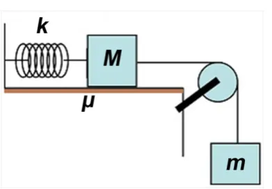
Our system consists of a spring (spring’s constant k), on a horizontal table with

coefficient of kinetic friction µ, which is fixed at one end and the other end is

attached to a block of mass M which is connected to a massless rope that passes

over a frictionless pulley fixed (but free to rotate) at the end of the table and

another block of mass m attached to the rope and hanged off the table (see

Fig-ure 1 below).

Initially, the system is at rest and the zero reference is set at the position of m.

After the system is released, the maximum downward distance, x0 covered by

m occurs when it comes momentarily to rest and this can be determined by

re-quiring that the work done by frictional force is equal to the change in the me-chanical energy, with the result;

(

)

0 2

x mg Mg

k µ

= − . (1)

This occurs when m reaches zero velocity and M reaches maximum

displace-ment to the right. In the second step m returns up and M moves to left until the

system gets to zero velocity after which M moves to right and m moves

down-ward and the system repeats the motion with decreasing amplitude due to the

work done by frictional force between M and the table. Finally the system comes

to final stable equilibrium state and the final displacement xf made by the

(3)

[image:3.595.283.479.64.200.2]

Figure 1. Two masses connected to a spring.

(

)

1

f

x mg Mg

k µ

= − , (2)

which is exactly half x0. We must note that initially (just before the release) the

system is in a non-equilibrium state and finally in an equilibrium state. The dy-namics which controls the behavior of the system between these two states is undermined and the physics involved is not utilized. Our aim in this paper is to examine the behavior of the system during its transition between these two states. Specifically, we will find the position of m during any given half cycle n, its final position at the end of each half cycle and the number of half cycles made by the system before it comes to the final equilibrium state.

Let x be a generalized coordinate, the Lagrangian of the system is

(

)

2 2

1 1

2 2

L= m M x+ −_ kx −mgx_

 

 , (3)

where x and x are the position and speed of m. The Lagrange’s equation of

motion for the generalized coordinate x reads

d d

L _{L Q}

t x x

∂ ∂

 _{ − =}

_∂  _∂

  , (4)

where Q is the frictional force between the surface and M and is given by

( )

1n

Q= − µMg_{, (5)}

with n is the number of half-cycle of the motion. For odd n, M is moving to the

right so that the frictional force is negative, while for even n, M is moving to the left so that the frictional force is positive. Inserting Equations (4) and (5) into Equation (3) gives

( )

(

)

2 1 ₁n

x x mg Mg

m M

ω µ

+ = + −

+

 , (6)

where _{ω =}2 _{k m M}

(

₊

)

_{. Equation (6) is an inhomogenous first order}

differen-tial equation, whose solution after applying the inidifferen-tial condition xn=0 for

each half-cycle, is

( )

1

(

( )

)

cos 1n

n n

x A t mg Mg

k

ω µ

(4)

The constant An can be found as follows:

For the first half cycle,

( )

0,π , i.e. n=1, we have x1

( )

0 =0 so that equation (7)

gives A1=1_k

(

−mg+µMg

)

. For the second half cycle,

(

π,2π

)

, i.e. n=2, we

require that the final position of m at end of the first half cycle equals the initial position at the beginning of the second half cycle, which means the

( )

1 π 2 π

x =x . This gives, A2= = −1_k

(

mg+3µMg

)

. In a similar way, for the nth

half cycle,

(

n−1

)

π,nπ

)

_{, we require the position of}_m_{at end of the (}_n_{− 1) half}

cycle equals to its position at the beginning of the nth_{half cycle, which means}

(

)

(

)

(

)

1 1 π 1 π

n n

x− n− =x n− . One might expect that

(

)

(

)

1 ₂ ₁

n

A mg n Mg

k µ

= − + − , (8)

d hence Equation (7) becomes

(

)

(

)

(

( )

)

1 ₂ ₁ _cos 1 ₁ n

n

x mg n Mg t mg Mg

k µ ω k µ

= − + − + + − , (9)

which we prove by mathematical induction as follows: For n=1, we already

de-rived A1 which upon its substitution into Equation (7) gives x1. We assume

Equation (9) is true for any n, and we need to show that it is true for n+1. For

the

(

n+1

)

th_{half cycle,}

(

n nπ,

(

+1

)

π

)

_{, we require that} x nn

( )

π =xn+₁

( )

nπ . This

means that, at

ω

t n= π_{, the position of}_m_{at the end on the}_nth_{half cycle is equal}

to its position at the beginning of the

(

n+1

)

th_{half cycle. Using Equations (7)}

and (9), we get

(

)

(

)

( )

(

( )

)

( )

(

( )

)

1

2 1 cos π 1

cos π 1

n

n n

g _m _n _M _n g _m _M

k k

g

A n m M

k

µ µ

µ

+

− + − + + −

= + + −

The above equation immediately yields, for both case n = odd and n = even,

1 n

A+ , namely

(

)

(

)

1 1 2 1

n

A mg n Mg

k µ

+ = − + + , (10)

which, upon its substitution into Equation (7), gives us

(

)

(

)

( )

(

( )

1

)

1 1 2 1 cos 1 1

n n

x mg n Mg t mg Mg

k µ ω k µ

+

+ = − + + + + − . (11)

This is exactly xn given in Equation (9) with n→ +n 1, and this completes

the proof.

Equation (9) yields for n = odd, with

ω

t n= π

(

)

2

n

x mg n Mg

k µ

= − (12)

which gives the lowest position of m and the maximum right displacement of M

(5)

even, Equation (9) yields,

2

n n

x Mg

k µ

= _{, (13)}

which gives the highest position of m and the maximum left displacement of M

when they come momentarily to rest at the end of the nth_{half-even cycle.}

3. The Final Equilibrium State

Now the question is where the system comes to equilibrium permanently? We claim that this occurs at a final position given by

(

1

)

1 2

f n n

X = x +x+ . (14)

Using Equation (9) for xn, Equation (14) gives,

(

)

f

mg Mg

X

k

µ ±

= _{, (15)}

where the signs + (−) are for n = odd (even). The result given in Equation (15) is

expected, since for the n = odd case the motion is from odd n to even (n + 1)

which means that mass m is moving upward and M is moving to the to the left

and thus the balancing of forces gives mg+µMg kX= f which gives the result

in Equation (15) with the plus sign. Similarly, for the n = even case, motion is

from even n to odd (n + 1) which means that m is moving down and M is

mov-ing to the right and thus the balancmov-ing forces gives mg−µMg kX= f which

gives the result in Equation (15) with the negative sign.

It is interesting to find the value of n at which the system reaches its final

equilibrium state. This could be found by equating x nn

( )

π from Equation (9)

with Xf for the two cases n = even and n = odd which is given by Equation

(15). Straightforward calculations give, for both cases

1 ₁

2

m n

M

µ

 

= _ − _

  (16)

To find the total distance covered by either m or M, one must notices that for

the nth_{half-odd cycle}_m_{is moving down while for the}_nth_{half-even cycle it is}

moving up. Therefore, if we let N to be the integer part of Equation (16), we

have for N = even,

1

odd even

2 N 2 N

tot n n f

X =

∑

− x −

∑

x +X ₍₁₇₎

The substitution of xn for n = odd from Equation (12) and for n = even from

Equation (13) we get

(

)

1 1

odd odd even

2

4 ₁

4 ₂

2 2 4

N N N

tot f

f g

X m M n M n X

k

g _mN _M N N _N _X

k

µ µ

µ

− −

 

= _ − − _+

 

  

= _ − _ + + __+

  

 

∑

(6)

Substituting for Xf from Equation (15) with the negative sign, Equation (18)

gives

(

)

(

)

2 ₁

tot g g

X N m M N m M

k µ k µ

= _ − + _+ − . (19)

It is interesting to note that the substitution 1 1

2

m N

M

µ

 

= _ − _

  enables us to

write Equation (19) in terms of N or in terms of the original quantities as

(

)

(

2 2 2

)

2 ₁

2

tot g g

X MN N m M

k µ k Mµ µ

= + = − . (20)

Similarly, the total distance for the case N = odd, we have

2 1

odd even

2 N 2 N

tot n n f

X =

∑

− x −

∑

− x +X _{. (21)}

Noting that the two sums are similar to those in Equation (17) but with

1

N→N− , so using this and substituting for Xf from Equation (15) with the

positive sign, we get

(

)(

)

2 ₁ ₁

tot g g m

X N m M M

k µ kµ µM

 

= − − + _ + _

 , (22)

which upon using m 2N 1

M

µ = + , the above equation can be written in terms of

N or in terms of the original quantities as

(

)

(

2 2 2

)

2 ₁

2

tot g g

X MN N m M

k µ k Mµ µ

= + = − _{. (23)}

This is exactly the same as the total distance given by Equation (20) for the even N case.

It is constructive to express the total distance Xtot in terms of the final position

f

X . For N = even, Equation (15) gives Xf = g_k

(

m−µM

)

= g_kµM N

( )

2 , so that

2g M Xf

k µ = N . Substituting this in Equation (20) gives

(

1

)

tot f

X = N+ X . (24)

while for N = odd, Equation (15) gives Xf g_k

(

m M

)

2g M_k

(

N 1

)

µ µ

= + = + , so

that 2

1

f X g M

k µ = N+ . Substituting this result into Equation (23) gives

tot f

X =NX ₍₂₅₎

4. Energy Considerations

Our result for the total distance covered by m or M can be checked from energy

considerations. The gravitational potential energy of m is consumed by energy

stored in the spring and a work done against friction between M and the surface.

(7)

2

1 2

f f tot

mgX = kX +µMgX (26)

Using Equation (15) for Xf, we get:

For N = even, 1 1 ( ) 1 1

2 2

tot f f m

X X mg g m M X

Mg µ M

µ µ

 

= _ − − _= _ + _

    and

using m 2N 1

M

µ = + , we recover our result given in Equation (24), namely

(

1

)

tot f

X =X N+ .

For N = odd, the substitution for Xf from Equation (15) into Equation (26),

we get 1 1

(

)

1 1

2 2

tot f f m

X X mg g m M X

Mg µ M

µ µ

 

= _ − + _= _ − _

    and using

2 1

m _N

M

µ = + , we recover our result given in Equation (24), namely, Xtot=NXf.

It is interesting to determine the energy stored in the spring, Us and the

work done against friction Wf and compare them with the initial gravitational

potential energy, Ug of the hanged mass m relative to its final position.

Using Equation (15) for Xf and Equation (20) for Xtot, we get

(

)

2

, even

g f mg

U mgX m M N

k µ

= = − = ₍₂₇₎

(

)

2

, odd

g mg

U m M N

k µ

= + = (28)

(

)

(

)

2 2 2 2 2 , 1 _even 2 2 , odd 2

s f g

U kX m M N

k g m M N

k µ µ = = − = = + = (29)

(

)

2

2 2 2 _, _{even or odd}

2

f tot g

W MgX m M N

k

µ µ

= = − = ₍₃₀₎

From the above equations, one can immediately find,

1 2

s

g

U m M

U m

µ ±

= _{, (31)}

where the − (+) sign is for N = even (odd)

1 2

f

g

W m M

U m

µ

±

= _{, (32)}

where the + (−) sign is for N = even (odd).

It is constructive and interesting to consider the special case when the

hori-zontal surface is frictionless (µ →0): Equations (27)-(29) give

2 2

g m g

U k

= _, 2 2

2

s f m g

U W

k

= = _{, (33)}

and therefore, 1 2 f s g g W U

(8)

So we observe that even when the system is non-dissipative, half the initial gravitational potential energy will be stored in the spring while the other half is lost.

5. Conclusion

In this paper, we examined the dynamics of a classical system during its transi-tion from a non-equilibrium state to a final equilibrium one. The positransi-tion of the

system at the end of the nth_{-half cycle was calculated. The even and odd half}

cycle was examined and our results for the final position are consistent with

force balancing for each parity of n. The number of half cycles is determined by

the masses of the connected blocks and the coefficient of kinetic friction. Fur-thermore, the total distance covered by the system was determined. The energy involved during the system’s transition was calculated for the two parity cases of

n. Our results show that in the limit of vanishing coefficient of friction the

ener-gy stored in the spring is exactly half the initial gravitational potential enerener-gy and the other half is an energy loss. This is in complete analogy with the energy loss in the two-capacitor problem.

Conflicts of Interest

The author declares no conflicts of interest regarding the publication of this pa-per.

References

[1] Cohen, E.G.D. (2015) On the Transition of a Non-Equilibrium System to an Equili-brium State. The European Physical Journal Special Topics, 224, 801-807. https://doi.org/10.1140/epjst/e2015-02428-5

[2] Berthier, L. and Kurcham, J. (2013) Non-Equilibrium Glass Transitions in Driven and Active Matter. Nature Physics, 9, 310-314. https://doi.org/10.1038/nphys2592 [3] Fenf, H., Zhang, K. and Wang, J. (2014) Non-Equilibrium Transition State Rate

Theory. Chemical Physics, 5, 3761.

[4] Nicolis, G. and Drigogine, I. (1971) Fluctuations in Non-Equilibrium Systems. Pro-ceedings of the National Academy of Sciences of the United States of America, 68, 2102-2107. https://doi.org/10.1073/pnas.68.9.2102

[5] Zia, R.K.P., Shaw, L.B., Schmittmann, B. and Astalos, R.J. (2000) Contrasts between Equilibrium and Non-Equilibrium Steady States: Computer Aided Discoveries in Simple Lattice Asses. Computer Physics Communications, 127, 23-31.

https://doi.org/10.1016/S0010-4655(00)00022-9

[6] Derrida, B. (2007) Non-Equilibrium Steady States: Fluctuations and Large Devia-tions of the Density and of the Current. Journal of Statistical Mechanics Theory and Experiment, 2007, Article ID: 07023.

https://doi.org/10.1088/1742-5468/2007/07/P07023

[7] Odagaki, T. (2017) Non-Equilibrium Statistical Mechanics Based on the Free Ener-gy Landscape and Its Applications to Glassy Systems. Journal of the Physical Society of Japan, 86, Article ID: 082001. https://doi.org/10.7566/JPSJ.86.082001

(9)

Industrial Research, 67, 747-758.

[9] Rabani, E. and Berne, B.J. (1998) Energy Dissipation in Non-Linear Systems Coupled to a Bath: On the Use of Perturbative Maps. Journal of Physical Chemistry A, 102, 9380-9389. https://doi.org/10.1021/jp9814653

[10] Xiong, Y, Wang, T. and Teng, P. (2016) The Effect of Dissipation on Topological Mechanical Systems. Scientific Reports, 6, Article ID: 43572.

https://doi.org/10.1038/srep32572

[11] Perieversev, A., Pereversev, Y. and Prezhodo, O.V. (208) Dissipation of Classical Energy in Non-Linear Quantum Systems. Journal of Chemical Physics, 128, Article ID: 134107.

[12] Ghadirian, R., Stait-Gardner, T., Hennessy, A. and Price, W.S. (2011) Energy Dissi-pation in Porous Media for Equilibrium and Non-Equilibrium Translational Mo-tion. Journal of the Basic Principles of Diffusion Theory Experiment and Applica-tions, 15, 1-21.

[13] Bonanca, M.V.S. and de Aquiar, M.A.M. (2006) Equilibrium via Interaction with Chaotic Systems. Physica A, 365, 333-340.

https://doi.org/10.1016/j.physa.2005.09.062

[14] AL-Jaber, S.M. and Salih, S.K. (2000) Energy Considerations in the Two-Capacitor Problem. European Journal of Physics, 21, 341.

https://doi.org/10.1088/0143-0807/21/4/307

[15] Mita, K. and Boufaida, M. (1999) Ideal Capacitor Circuits and Energy Conservation.

American Journal of Physics, 67, 737-738. https://doi.org/10.1119/1.19363

[16] Choy, T.C. (2004) Capacitors Can Radiate: Further Results for the Two-Capacitor Problem. American Journal of Physics, 72, 662-670.

https://doi.org/10.1119/1.1643371

[17] Timothy, B.B., Hite, D. and Singh, N. (2002) The Two-Capacitor Problem with Radiation. American Journal of Physics, 70, 415-420.

https://doi.org/10.1119/1.1435344

[18] Abu-Labdeh, A.M. and AL-Jaber, S.M. (2008) Energy Consideration from Non-Equilibrium to Equilibrium State in the Process of Charging a Capacitor.

Journal of Electrostatics, 66, 190-192.https://doi.org/10.1016/j.elstat.2007.12.002 [19] AL-Jaber, S.M. and Abu-Labdeh, A.M. (2011) Energy Consideration in the Process

of Transition to Equilibrium State. Natural Science, 3, 136-140.

https://doi.org/10.4236/ns.2011.32019

[20] Lee, K. (2009) The Two-Capacitor Problem Revisited: A Mechanical Harmonic Os-cillator Model Approach. European Journal of Physics, 30, 69-74.

https://doi.org/10.1088/0143-0807/30/1/007

[21] Lara, V.O.M., Lima, A.P. and Costa, A. (2015) Entropic Considerations in the Two-Capacitor Problem. Revista Brasilean de Ensino de Fisica, 37, 1301-1306.

https://doi.org/10.1590/S1806-11173711650

[22] Libii, J.N. (2009) Demonstration of Energy Dissipation in a Spring-Mass System Undergoing Free Oscillations in Air. World Transactions on Engineering and Technology Education, 7, 28-33.

[23] Nijmeijera, H. (2004) Energy Dissipation of a Friction Damper. Journal of Sound and Vibration, 278, 539-561.https://doi.org/10.1016/j.jsv.2003.10.051

(10)

DOI: 10.4236/am.2018.98062 906 Applied Mathematics [25] Krim, J. (2012) Friction and Energy Dissipation Mechanisms in Adsorbed

Mole-cules and Molecularly Thin Films. Advances in Physics, 61, 155-323.

https://doi.org/10.1080/00018732.2012.706401

[26] Onorato, P., Mascoli, D. and Deambrosis, A. (2010) Damped Oscillations and Equi-librium in a Spring-Mass System Subjected to Sliding Friction Forces: Integrating Experimental and Theoretical Analysis. American Journal of Physics, 78, 1120-1126.https://doi.org/10.1119/1.3471936

[27] Besson, U., Borghi, L., De Ambrosis and Mascheretti, P. (2007) How to Teach Fric-tion: Experiments and Models. American Journal of Physics, 75, 1106-1113.

https://doi.org/10.1119/1.2779881

[28] Molina, M.I. (2004) Exponential versus Linear Amplitude Decay in Damped Oscil-lators. Physics Teacher, 42, 485-487.https://doi.org/10.1119/1.1814324