Research on the Relationship between Entrepreneur Confidence Index and Producer Price Index Based on Quantile Granger Causality

ISSN Online: 2327-5960 ISSN Print: 2327-5952

DOI: 10.4236/jss.2018.610006 Oct. 23, 2018 54 Open Journal of Social Sciences

Research on the Relationship between

Entrepreneur Confidence Index and

Producer Price Index Based on Quantile

Granger Causality

Qiying Lao

*

_{, Guoqiang Tang, Huifang Qu}

College of Science, Guilin University of Technology, Guilin, China

Abstract

This paper investigates the relationship between Entrepreneur Confidence Index and Producer Price Index (PPI) based on the mean and quantile Gran-ger causality tests, using quarterly statistics data from 2005 to 2017. The re-sults indicate that there is a unidirectional causality between entrepreneur confidence index and PPI index. At different quantile levels, entrepreneur confidence index of the previous period has different effects on the current PPI index. At lower quantiles, the causality from entrepreneur confidence index to PPI index is significant, while entrepreneur confidence index has lit-tle impact on PPI at higher quantiles. The estimates of βˆ1 at low quantiles

are positive and significant. Therefore, improving entrepreneur investment confidence will have a certain positive impact on PPI.

Keywords

Entrepreneur Confidence Index, Producer Price Index, Quantile Regression, Granger Causality Test

1. Introduction

China’s economic development has entered a new normal at present, the re-gional economy and industrial structure have been continuously improved, and the economy operation maintains a steady and positive trend. Since the second half of 2016, entrepreneur confidence index constantly rallied and rose 4.5% year-on-year in the first half of 2016, the production and development market is active, and the efficiency of enterprises is improved. Entrepreneurs think that How to cite this paper: Lao, Q.Y., Tang,

G.Q. and Qu, H.F. (2018) Research on the Relationship between Entrepreneur Confi-dence Index and Producer Price In-dex-Based on Quantile Granger Causality. Open Journal of Social Sciences, 6, 54-67. https://doi.org/10.4236/jss.2018.610006

Received: September 14, 2018 Accepted: October 20, 2018 Published: October 23, 2018

Copyright © 2018 by authors and Scientific Research Publishing Inc. This work is licensed under the Creative Commons Attribution International License (CC BY 4.0).

DOI: 10.4236/jss.2018.610006 55 Open Journal of Social Sciences current macro-control policy will have a positive effect on future economy. Chi-na’s producer price index rose 6.4% year-on-year over the period January 2017 to July; China has achieved a good momentum while at the same time securing progress in its economic development. This may be related to market partici-pant’s expectations of economic conditions in the future and good prospects of the economy. Entrepreneurs are the leaders of enterprise production and opera-tion, whose performance and behavior often play a vital role, influencing eco-nomic development significantly. In the General Theory of Employment, Interest, and Money [1], Keynes pointed out that when people were confident about the future economic development, they would increase investment to expand the scale of production and operation; when people lacked confidence in the future economic development, they would reduce production capacity to minimize the losses, thereby inhibiting investment and consumption. Therefore, market con-fidence will affect the economic development by influencing the deci-sion-making of economic actors. With the above in mind, this paper takes pro-ducer price index (PPI) as the research object, and adopts the quarterly entre-preneur confidence index as the measurement index of entreentre-preneur confidence, which is published by Oriental Fortune Net. We analyze and empirically investi-gate the relationship between entrepreneur confidence and PPI to provide cor-responding policy suggestions for improving the confidence of entrepreneurs and forecasting the trend of economic development.

DOI: 10.4236/jss.2018.610006 56 Open Journal of Social Sciences equilibrium relation with PPI [12]. Nie et al. (2017) established the VAR model to measure the relationship among China’s agricultural product price index, PPI and economic growth [13]. Luo et al. (2018) used VAR-VEC model to analyze the relationship between consumer confidence index (CCI) and PPI [14].

Previous studies are more common to test non-causality in conditional mean based on a linear model, it reveals the average influence in different economic variables, while cannot depict the influence at other places, we are therefore mo-tivated to characterize and test causal relations in other conditional distribution characteristics. In this paper, we analyze the effect of entrepreneur confidence index on PPI index using both the mean and quantile Granger causality tests, and the causal relations between them were discussed. The rest of the study is organized as follows. We introduce the notion of Granger causality in mean and quantiles in Section 2. The empirical results of different causal models are pre-sented in Section 3. Section 4 concludes the study.

2. Empirical Methodology

2.1. Mean Granger Causality Test

Granger (1969) proposed a causal relation based on prediction [15], which mainly examined whether the explanatory variable X was in favor of predicting Y, if X and its lag values were increased, the prediction ability of Y conditional mean could be significantly enhanced. We define that X is the Granger cause of Y, call it X ⇒Y_{. Otherwise, we say that X is not the Granger cause of Y and}

call it X⇒/ Y. The Granger causality is used as the null hypothesis by defining non-causality between variables, namely,

(

)

1

[

1

]

| , |

t t

y t y t

F _η Y X ₋  =_ F η Y_{− ,} ∀ ∈η IR ₍₁₎

where F_yt

[ ]

⋅|F is the conditional distribution of yt, and

(

Y X,

)

t−1 is the

in-formation set generated by yi and xi up to time t − 1. The variable X is said to

Granger causes Y when Equation (1) fails to hold. As estimating and testing con-ditional distribution are practically cumbersome, it is more common to test a necessary condition of (1), namely,

(

)

1

[

1

]

| , |

t t t t

E y Y X − = E y Y−

(2)

where E y F

[

_t|

]

is the mean of F_yt

[ ]

⋅|F _{. We say that X does not Granger}

cause Y in mean if (2) holds; otherwise, X Granger causes Y in mean.

In order to test whether the entrepreneur confidence index (QYJ) is the mean Granger cause of PPI index, we consider null hypothesis H QYJ0: ⇒/ PPI or

0: 1 q 0

H

β

==

β

= , the two unconstrained and constrained mean regression models are needed to be built:

(

)

0

1

p

t i t i

i

E PPI a αPPI−

=

= +

∑

(3)

(

)

0

1 1

p q

t i t i j t j

i j

E PPI a

α

PPI−

β

QYJ−

= =

DOI: 10.4236/jss.2018.610006 57 Open Journal of Social Sciences where PPIt is the producer price index at time t, i is the lag order of producer

price index, p is the maximum lag order of producer price index, QYJt is the

entrepreneur confidence index at time t, j is the lag order of entrepreneur confi-dence index, q is the maximum lag order of entrepreneur confidence index,

t j

QYJ− is the entrepreneur confidence index at time (t j− ), a0 is constant

term. Equation (3) is a constrained mean regression model, which indicates that QYJ has no significant influence on PPI; Equation (4) is a unconstrained mean regression model, the independent variable of the model depends on the lagged values of PPIt and QYJt, which indicates QYJ has a significant effect on PPI.

We construct F test statistics according to the residual sum of squares of both constrained and unconstrained mean regression models, namely,

(

)

(

)

(

(

)

)

1 2 2

, 1

1

ESS ESS p

F F p T q p

ESS T q p

−

= − + +

− + +

 

  (5)

where ESS1 is the residual sum of squares of constrained model, ESS2 is the

residual sum of squares of unconstrained model. If the statistic F F> a (a is a

confidence), then we reject the null hypothesis and it can be considered that QYJ is the mean Granger cause of PPI, otherwise the null hypothesis is accepted.

When using Granger causality, time series are required to be stationary or non-stationary with cointegration relations, otherwise the results will be wrong. In addition, as causality test is sensitive to lag order, several lag orders are usually tested in actual experiment. If the test results are consistent, the results are con-sidered to be more reliable.

2.2. Quantile Granger Causality Test

The mean Granger causality test is limited to test the causal relations between the mean value of explanatory variable on the conditional distribution of response variable, and it is unable to describe its predictive ability of response variable at other places. The quantile Granger causality test can make up for this deficiency. By combining the quantile regression with the mean Granger causality test, it can find the specific location where the causal relationship between variables is es-tablished, so as to catch the casual relationship that cannot be found by the mean Granger causality test. Therefore, other conditional distribution characters are considered to test the causal relationship. The quantile Granger causality not on-ly can test the causality on the mean value of conditional distribution, but also can test the causality of variables on different conditional quantiles, it can fully describe the overall picture of the conditional distribution of response variables. And the quantile regression does not require a strong hypothesis for the error term, so the estimator of quantile regression coefficient is more robust for the non-normal distribution.

DOI: 10.4236/jss.2018.610006 58 Open Journal of Social Sciences

(

)

1

[

1

]

| , |

t t

y t y t

Q τ Y X −  =Q τ Y− , ∀ ∈τ

( )

0,1 ₍₆₎

We say that X does not Granger cause Y in all quantiles if (6) holds. We may define Granger non-causality in a quantile range

( ) ( )

b c, ⊂ 0,1 _as

(

)

1

[

1

]

| , |

t t

y t y t

Q τ Y X − =Q τ Y− , ∀ ∈τ

( )

b c, (7)

To test whether X is the quantile Granger cause of Y, the linear quantile re-gression model is established as follow:

( )

( )

( )

( )

( )

( )

0 1, 1, 1

t t p t q t t t

y a= τ +α τ y′₋ +β τ x′₋ + τ =z′₋θ τ + τ ₍₈₎

where

θ τ

( )

a0

( ) ( ) ( )

τ α τ

, ,

β τ

′

 ′ ′

= _ _ is the k-dimensional parameter vector

with k= + +1 p q_{, and t}

( )

τ _{is the corresponding error.}

Given a linear model for conditional quantiles, testing (6) amounts to testing

( )

0: 0

H β τ = , ∀ ∈τ

( )

0,1 (9)

For a given τ _{, it can be derived the Wald statistic of} β τ

( )

=0 _through Equ-ation (8), that is:

( ) ( )

(

₍

)

₎

( )

1 1 ˆ2

ˆ ˆ ˆ

1

zz

T T

T

T M f

W τ τ τ

β ψ ψ β

τ τ

− −

′ ′

=

− (10)

where

β

ˆT( )τ is the estimate of β τ

( )

, ψ is a selection matrix, and the formula

( )

( )

ψθ τ =β τ is hold, 1 1 1

1

ˆ T

zz t t

i

M Z Z

T − −

=

′

=

∑

, fˆ is probability density function.

To test (9), Koenker and Machado (1999) suggested using a Sup-Wald test, the supremum of WT( )τ .

In what follows, let Bq denote a vector of q independent Brownian bridges, ⇒ _{denote weak convergence (of associated probability measures) and} ⋅

de-note the Euclidean norm. Clearly, Bq

( )

τ equals

(

)

( )

1 2

1 N 0,Iq τ −τ

 

  in

dis-tribution, and the formula as follow:

( )

( )

1 2

( )

ˆ D

T q

T_β τ −β τ _→Ω B τ (11)

Under suitable conditions, (11) holds uniformly on a closed interval Λ ⊂

( )

0,1 ; see Koenker and Machado (1999) for details. We then have, under the null hy-pothesis (9),

( )

( )

(

)

2 1 q T B

W τ τ

τ τ

⇒

− , τ ∈Λ

where the weak limit is the sum of squares of q independent Bessel processes. This immediately leads to the following result:

( )

( )

(

)

2 sup sup 1 q T B W τ τ τ τ τ τ

DOI: 10.4236/jss.2018.610006 59 Open Journal of Social Sciences ANDREWS [17] and KOENKER [18] calculated the critical values of sup-Wald statistics according to the simulation method. Table 1 presents the simulated critical values of sup-Wald test (with q = 1, 2) on [0.05, 0.95].

3. Empirical Study

3.1. Data Description

Entrepreneur confidence index (QYJ) reflects entrepreneur’s feeling and confi-dence in macroeconomic environment, it is an indicator to forecast the changing trend of economic development. The value is between 0 and 200 with 100 as the critical value, a reading above 100 indicates a rise in confidence, the economy is in a state of prosperity. While one below 100 suggests that confidence has de-creased, the economy is in recession. The PPI is the barometer of national eco-nomic conditions, which reflects the prosperity and depression of the economy. In order to intuitively understand the changing relationship between entrepre-neur confidence index and PPI index over years, this paper collects quarterly sta-tistical data from the first quarter 2005 to the fourth quarter 2017, the changing trend of the entrepreneur confidence index and PPI index is plotted from the data, as shown in Figure 1.

[image:6.595.208.542.434.707.2]

As can be seen from Figure 1, the volatility of the entrepreneur confidence index during the sample period is greater than that of the PPI index, but the changing trend of entrepreneur confidence index is basically consistent with PPI index. That is, the entrepreneur confidence index rises and the PPI rises, conversely,

Table 1. Critical values of sup-Wald test (q = 1, 2).

q α = 0.1 α = 0.05 α = 0.01

1 8.19 9.84 13.01

2 11.20 12.93 16.44

[image:7.595.228.523.418.703.2]

DOI: 10.4236/jss.2018.610006 60 Open Journal of Social Sciences the entrepreneur confidence index falls and so does PPI. The changes between the two series can be mainly divided into three parts: one is from 2005 to the end of 2007, China’s economy is overheating in this period, and both entrepreneur confidence index and PPI index are running at a high level, the entrepreneur confidence index is much higher than 100, indicating that enterprises are posi-tive and optimistic about the current economic situation and future expectation. Macroeconomic investment rises and the economy has entered a rapid growing stage; Two is from 2008 to 2010, influenced by international financial crisis and in the economic downturn, entrepreneurs lack confidence in investment. China’s eco-nomic development has received a greater negative impact, especially in the fourth quarter of 2008, the entrepreneur confidence index is always below 100; Three is the post-crisis from 2010 to 2017, the government has issued a series of economic poli-cies to strengthen domestic and foreign investment to stimulate economic growth. The confidence of enterprise investors has gradually recovered. However, due to the lack of technological innovation capacity, structural industry surplus and other problems, the growth momentum of China’s economic development is not strong, and the entrepreneur confidence index has dropped significantly.

Figure 2 and Figure 3 depict the normality test results of the PPI index series.

In Figure 2, the histogram shows obvious bimodal characteristics, which

indi-cates that the PPI index series is not normal distribution, and there is a large deviation between its kernel density curve (solid line) and normal density curve (dotted line). The upper tail of the Q-Q diagram deviates significantly from the

[image:8.595.206.541.80.380.2]

DOI: 10.4236/jss.2018.610006 61 Open Journal of Social Sciences

Figure 3. Q-Q diagram of PPI.

line In Figure 3, we, therefore, reject the assumption that the PPI index series follows normal distribution. This result shows that the precondition for mean regression model based on the classical assumption is no longer true. For this purpose, we need to establish a linear quantile regression model to explore the relationship between entrepreneur confidence index and PPI index.

3.2. Data Source and Processing

To study the causality between the entrepreneur confidence index and PPI index, the quarterly data from 2005 to 2017 are selected as variables. Among them, the entrepreneur confidence index (denoted as QYJ) is obtained from Oriental For-tune Net (http://www.eastmoney.com/), the logarithmic form is expressed by LNQYJ, and the first order difference is DLNQYJ. The PPI index data is obtained from National Bureau of Statistics (http://data.stats.gov.cn/), the seasonal average of PPI is expressed as LNPPI in logarithmic form and DLNPPI in first difference. Besides, in order to eliminate the effect of heteroscedasticity on regression results and reduce volatility, the data used in the empirical part were all taken with the natural logarithm, and the transformation of natural logarithm will not change the characteristics of the original data.

3.3. Unit Root Test

stationar-DOI: 10.4236/jss.2018.610006 62 Open Journal of Social Sciences ity of the series. Checking for stationarity of data series is an important prerequi-site in most empirical time series analysis, as these methods require stationarity of the variables. Results of unit root test are reported in Table 2. The results show that ADF statistics of LNQYJ and LNPPI are more than the critical values of 1%, 5% and 10%, and the p-values are also more than 0.05, so we cannot reject the null hypothesis of unit roots for both variables in level form. However, the null hypothesis is rejected when ADF unit root test is applied to the first differences of each variable. The first differences of the QYJ and PPI are stationary indicat-ing that these variables are integrated of order one, I (1).

3.4. Cointegration Test

The purpose of cointegration test is to prevent spurious regression. There are two theories to test the cointegration relationship of time series. One is En-gle-Granger (E-G) two step method, the other is Johansen test based on VAR model. This paper uses E-G two step method to test the cointegration relation-ship between LNQYJ and LNPPI series. The E-G two step method is to conduct unit root test of regression residual series based on OLS model. Firstly, we apply OLS to fit equation yt= +α βxt+µt, and the regression equation is used to

calculate the non-equilibrium error µˆ_{t; then the stationarity of residual series} ˆt

µ is tested. If µˆt is a stationary series, it is considered that xt and yt are

cointegration variables, and there is a long-run equilibrium relationship between them. As Engle and Granger (1987) pointed out, only non-stationary variables with the same order of integration could be tested for cointegration. Since QYJ and PPI series are integrated with the same order I (1), cointegration test can be conducted by E-G two step method.

By using OLS estimation, the cointegration regression equation is

(

) (

)

LNPPI 85.37 0.13LNQYJ 21.50062 3.404283

t µ

= + +

(13)

[image:9.595.207.541.622.738.2]

The t statistics of each parameter are shown within parentheses in Equation (13), the adjusted R-squared is 0.865107, the F-statistics is 75.35606, the p-values of the constant term C and the explanatory variable LNQYJ are 0.0000 and 0.0014 respectively, both of which are less than 0.05. It can be seen from the re-gression results that the fitting effect of the cointegration rere-gression equation is very good.

Table 2. Results of ADF unit root test.

Series ADF test _value Critical value P value Conclusion

1% 5% 10%

LNQYJ −2.785002 −3.56831 −2.9212 −2.898551 0.0676 Non-stationary LNPPI 0.019370 −2.61301 −1.9477 −1.612573 0.6842 Non-stationary

DLNQYJ −5.906184 −2.61203 −1.9475 −1.61265 0.0001 stationary

DOI: 10.4236/jss.2018.610006 63 Open Journal of Social Sciences And then the unit root test is performed on the estimated residual series µˆt.

The critical value applied by ADF test during the cointegration analysis is differ-ent from the traditional ADF test, but refers to the table of cointegration critical values provided by Engle-Granger. The equation for calculating critical value is

( )

1 2

1 2

C α φ φT− φT−

∞

= + + , Where T represents the sample size and α is the significance level. According to Equation (13), the critical value C

( )

α _is

−3.3410 at the given α =0.05. When conducting ADF test of residual series, the test statistic is −4.531120, which is less than the critical value at α =0.05_{. The}

result shows that we can reject the null hypothesis. Therefore, the residual series is stationary. So we have reasons to believe that, there is a cointegration ship between LNQYJ and LNPPI, and there is a long-run equilibrium relation-ship between the entrepreneur confidence index and PPI index. In the long-run, every 1% rise in entrepreneur confidence index is associated with increases of 0.13% in PPI index.

Based on the above ADF test and E-G cointegration test, we find that the en-trepreneur confidence index and PPI index are both non-stationary time series, and there is a long-run equilibrium relationship between the two series, thus it is suitable for the two economic variables to analyze their relationship by using Granger causality test.

3.5. Mean Granger Causality Test

[image:10.595.210.540.597.726.2]

The Granger causality test is used to analyze the causal relationship between the variables’ conditional mean, which is to test whether the explanatory variable X is favorable for predicting the behavior of the prerequisite is that X and Y are sta-tionary series or non-stasta-tionary series with cointegration relations. Granger pointed out that if two integral series with the same order had cointegration rela-tionship, there must be causality to support this long-run equilibrium, and the influence might be one-way or two-way. To explore the relationship between the entrepreneur confidence index and PPI index, the mean Granger causality test is performed on LNQYJ and LNPPI series. Since the optimal lag order of VAR is one, this paper chooses the mean Granger causality test of one lag order. In order to make the test results more reliable, the two lag order and three lag order are also tested. Table 3 presents the results of mean Granger causality test.

Table 3. Results of mean Granger causality test.

Null hypothesis Observation Lag order F-statistic P value Conclusion

LNPPIt → LNQYJt 51 1 3.61883 0.0631 accept

LNQYJt → LNPPIt 51 1 14.7861 0.0004 reject

LNPPIt → LNQYJt 50 2 0.94621 0.3958 accept

LNQYJt → LNPPIt 50 2 5.1057 0.01 reject

LNPPIt → LNQYJt 49 3 1.33439 0.276 accept

DOI: 10.4236/jss.2018.610006 64 Open Journal of Social Sciences From Table 3, at 5% level, the results show that the PPI index is not the Gran-ger cause of the entrepreneur confidence index, while reject the entrepreneur confidence index is not the Granger cause of PPI index. It indicates that the change in entrepreneur confidence index can cause the change in PPI index to some extent.

3.6. Quantile Granger Causality Test

For the quantile Granger causality test, the causality between variable LNPPIt and LNQYJt can be tested in two ways: one is to test a single coefficient, that is, the significance of the lag parameter of the independent variable is tested respec-tively. We considered the null hypothesisH0:βj=0

(

j=1,2, , q

)

. LNQYJt is considered as the Granger causal of LNPPIt if the hypothesis is not true at a cer-tain τ _{. The other is the joint test of all parameters, the null hypothesis is}

0: 1 q 0

H

β

=_=

β

= _{. LNQYJt is considered as the Granger causal of LNPPIt if}

the hypothesis is not true at all τ_.

3.6.1. Single Coefficient Test in Quantile

For each PPI-QYJ relation, we consider the following model:

( )

( )

( )

( )

1 1

p q

t i t i j t j t

i j

y

α τ

α τ

y−

β τ

x−

µ τ

= =

= +

∑

+

∑

+

₍₁₄₎

To determine whether PPI index Granger causes entrepreneur confidence in-dex, y is LNPPI and x is LNQYJ; for reversed causal relations, y is LNQYJ and x is LNPPI. This model specification allows us to investigate whether lagged x de-livers information (about y) that is not contained in lagged y.To illustrate, we es-timate model (14) with p q= =1 according to the optimal lag order of VAR. For each y, 19 quantile regressions (with

τ

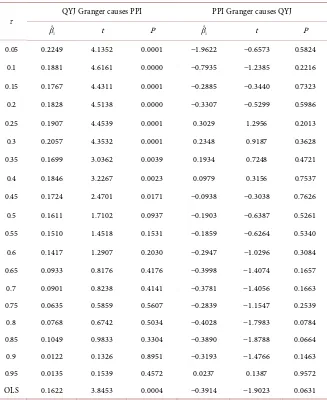
=0.05,0.1, ,0.9,0.95 ) least-squares regression (OLS) are computed. The results of Granger causality test in quantile are reported in Table 4.

The coefficient estimates βˆ1, the test statistics t and the p-values are provided

for this test. Table 4 shows the testing of whether PPI index Granger causes trepreneur confidence index. Since the p-values are greater than 0.05 across en-tire conditional distribution (when 0.05≤ ≤τ 0.95_{), it is evident that there is no}

causality from PPI index to entrepreneur confidence index, the result is the same as OLS test and the above mean Granger causality test. We conclude that PPI index changes do not lead entrepreneur confidence index changes in 0.05≤ ≤τ 0.95_.

When we test whether entrepreneur confidence index Granger causes PPI index, the p-values are significant and are all less than 0.05 in 0.05≤ ≤τ 0.45_{, hence}

there are strong reasons to accept that entrepreneur confidence index Granger causes PPI index at lower quantiles. However, when 0.5< ≤τ 0.95_{, it is not}

[image:12.595.211.538.87.487.2]

DOI: 10.4236/jss.2018.610006 65 Open Journal of Social Sciences

Table 4. Results of quantile Granger causality test.

τ QYJ Granger causes PPI PPI Granger causes QYJ

1

ˆ

β t P βˆ1 t P

0.05 0.2249 4.1352 0.0001 −1.9622 −0.6573 0.5824

0.1 0.1881 4.6161 0.0000 −0.7935 −1.2385 0.2216

0.15 0.1767 4.4311 0.0001 −0.2885 −0.3440 0.7323

0.2 0.1828 4.5138 0.0000 −0.3307 −0.5299 0.5986

0.25 0.1907 4.4539 0.0001 0.3029 1.2956 0.2013

0.3 0.2057 4.3532 0.0001 0.2348 0.9187 0.3628

0.35 0.1699 3.0362 0.0039 0.1934 0.7248 0.4721

0.4 0.1846 3.2267 0.0023 0.0979 0.3156 0.7537

0.45 0.1724 2.4701 0.0171 −0.0938 −0.3038 0.7626

0.5 0.1611 1.7102 0.0937 −0.1903 −0.6387 0.5261

0.55 0.1510 1.4518 0.1531 −0.1859 −0.6264 0.5340

0.6 0.1417 1.2907 0.2030 −0.2947 −1.0296 0.3084

0.65 0.0933 0.8176 0.4176 −0.3998 −1.4074 0.1657

0.7 0.0901 0.8238 0.4141 −0.3781 −1.4056 0.1663

0.75 0.0635 0.5859 0.5607 −0.2839 −1.1547 0.2539

0.8 0.0768 0.6742 0.5034 −0.4028 −1.7983 0.0784

0.85 0.1049 0.9833 0.3304 −0.3890 −1.8788 0.0664

0.9 0.0122 0.1326 0.8951 −0.3193 −1.4766 0.1463

0.95 0.0135 0.1539 0.4572 0.0237 0.1387 0.9572

OLS 0.1622 3.8453 0.0004 −0.3914 −1.9023 0.0631

PPI index, while this test is only conducted at a mean level and does thus not provide an overall picture of the existing causality from entrepreneur confidence index to PPI index. Quantile Granger causality test can provide the influence of entrepreneur confidence at different quantiles. Through this test, we not only look at the causality beyond the mean estimates, but we also account for the structural breaks.

It can be seen form Table 4 that the regression estimates of βˆ1 vary with

quantiles. The values of βˆ1 at lower quantiles are greater than that at higher

quantiles. They are significantly positive for lower quantiles but insignificant at higher quantiles (τ in [0.5, 0.95]). This implies that, the effect of entrepreneur confidence on PPI has an obvious difference when PPI is in different periods. For the PPI index at low quantiles, the estimates of βˆ1 on the previous

DOI: 10.4236/jss.2018.610006 66 Open Journal of Social Sciences

3.6.2. Joint Test in Quantiles

To be sure, this paper applies the sup-Wald test to check joint significance of βˆ1

on [0.05, 0.95]. We first test the Granger causality from entrepreneur confidence index to PPI index, the sup-Wald statistic is 10.3 and reject the null hypothesis of estimate β =1 0 at 5% level, this indicates that entrepreneur confidence

Gran-ger cause PPI. We then analyze the causality from PPI index to entrepreneur confidence index, the sup-Wald statistic is 5.6 and cannot reject the null hypo-thesis of estimate β =1 0 at 5% level, thus there is no evidence to believe that

the PPI index is the Granger causality for entrepreneur confidence index. The results of the joint test are the same as the single coefficient test, except that the single coefficient test know the causality in which areas of the quantile.

4. Conclusion

In this study, cointegration, and methodology of Granger causality test are em-ployed to empirically investigate causal link between entrepreneur confidence index and PPI index in China. We make use of quarterly data from the first quarter 2005 to the fourth quarter 2017. The cointegration test results indicate that there is a long-run equilibrium relationship between the entrepreneur con-fidence index and PPI index. And in the long-run, every 1% rise in entrepreneur confidence index is associated with increases of 0.13% in PPI index. Both the mean and quantile causality test indicate a one-way causality between the entre-preneur confidence index and PPI index. The direction of causality is from en-trepreneur confidence index to PPI index. The impact of enen-trepreneur confi-dence on PPI varies with quantiles. At lower quantiles, the causality from entre-preneur confidence index to PPI index is significant, and plays a positive role in promoting PPI. While entrepreneur confidence index has little impact on PPI at higher quantiles. The estimates of βˆ1 at low quantiles are positive and

signifi-cant. The results indicate that improving entrepreneur investment confidence will have a certain positive impact on PPI. When analyzing whether PPI index is the causality for entrepreneur confidence index, the p-values are not significant either in the mean test or in the quantile test. It fails to pass the significant test at the 5% level. The result indicates that PPI index is not the Granger causality for entrepreneur confidence index.

Conflicts of Interest

The authors declare no conflicts of interest regarding the publication of this pa-per.

References

[1] Cairns, M. and Xu, Y.N. (1963) General Theory of Employment Interest and Cur-rency. Commercial Press, 55-60.

[2] Xu, K. and Zhang, D. (2010) Forecasting Manufacturing Entrepreneur Confidence Index Based on GM (1, 1) Model. Statistics and Management, No. 2, 59-60.

En-DOI: 10.4236/jss.2018.610006 67 Open Journal of Social Sciences gineering, No. 8, 112-113.

[4] Liu, E.M. (2015) The Test of Priority of Entrepreneur Confidence Index and Busi-ness Climate Index. Bulletin of Science and Technology, No. 9, 20-24.

[5] Cheng, J.H. and Xu, K. (2015) Forecast and Analysis of Three Major Indices in 2015 under the New Economic Normal. Price: Theory & Practice, No. 1, 73 -75.

[6] Dong, D.Y. and Liu, K.Y. (2016) Forecast and Analysis of the Producer Price Index Based on ARIMA Model. Statistics & Decision, No. 1, 179-181.

[7] Luo, X.Q., Bao, Q., Wei, Y.J., et al. (2018) A Multivariate-Transmission-Based New Approach for Forecasting China’s Price Indexes in 2018. Management Review, No. 1, 3-13.

[8] Pan, J.C. and Tang, S.L. (2010) How Confidence Affect Inflation in China. Statistical Research, 27, 25-32.

[9] Qian, L. (2016) Research on the Influence of Entrepreneur Confidence Index on PMI-Based on Quantile Regression. Price: Theory & Practice, No. 10, 109-111. [10] Gui, W.L. and Li, Q.Y. (2017) Structure Analysis and Transmission Mechanism of

the Relationship between PMI and PPI Based on EEMD-JADE. The Journal of Quantitative & Technical Economics, No. 4, 110-128.

[11] Song, Y. and Wei, Z.Z. (2016) Research on the Driving Factors of Market Confi-dence in China-Based the Perspective of Consumer ConfiConfi-dence and Entrepreneur Confidence. Price: Theory & Practice, No. 8, 101-104.

[12] Shi, K. (2016) Analysis of Relationship between CPI and PPI Based on VEC Model. Statistics & Decision, No. 3, 83-86.

[13] Nie, G.H. and Zhou, Y.L. (2017) A Quantitative Research on the Relationship be-tween Economic Growth and the Agricultural Products Price Index & PPI in China. Journal of Shijiazhuang University of Economics, No. 3, 44-48.

[14] Luo, Y.N., Tang, G.Q. and Miu, Q.F. (2018) Research on the Relationship between CCI and PPI Based on VAR-VEC Model. Statistics & Decision, 34, 16-20.

[15] Granger, C.W.J. (1969) Investigating Causal Relations by Econometric Models and Cross-Spectral Methods. Econometrica, 37, 424-438.

https://doi.org/10.2307/1912791

[16] Chuang, C.C., Kuan, C.M. and Lin, H.Y. (2009) Causality in Quantiles and Dynam-ic Stock Return-Volume Relations. Journal of Banking & Finance, 33, 1351-1360. https://doi.org/10.1016/j.jbankfin.2009.02.013

[17] Andrews, D.W.K. (1993) Tests for Parameter Instability and Structural Change with Unknown Change Point. Econometrica, 61, 821-856.

https://doi.org/10.2307/2951764