ISSN Online: 2160-0384 ISSN Print: 2160-0368
DOI: 10.4236/apm.2018.88044 Aug. 20, 2018 720 Advances in Pure Mathematics
Extensions of the Constructivist Real
Number System
E. E. Escultura
GVP-Professor V. Lakshmikantham Institute for Advanced Studies, GVP College of Engineering, JNT University, Kakinada, India
Abstract
The paper reviews the most consequential defects and rectification of tradi-tional mathematics and its foundations. While this work is only the tip of the iceberg, so to speak, it gives us a totally different picture of mathematics from what we have known for a long time. This journey started with two teasers posted in SciMath in 1997: 1) The equation 1 = 0.99… does not make sense. 2) The concept i= –1 does not exist. The first statement sparked a debate that raged over a decade. Both statements generated a series of publications that continues to grow to this day. Among the new findings are: 3) There does not exist nondenumerable set. 4) There does not exist non-measurable set. 5) Cantor’s diagonal method is flawed. 6) The real numbers are discrete and countable. 7) Formal logic does not apply to mathematics. The unfinished debate between logicism, intuitionism-constructivism and formalism is re-solved. The resolution is the constructivist foundations of mathematics with a summary of all the rectification undertaken in 2015, 2016 and in this paper. The extensions of the constructivist real number system include the complex vector plane and transcendental functions. Two important results in the 2015 are noted: The solution and resolution of Hilbert’s 23 problems that includes the resolution of Fermat’s last theorem and proof Goldbach’s conjecture.
Keywords
Constructivism, Dark Number, Fermat’s Conjecture, g-Norm, g-Sequence, g-Limit, Goldbach’s Conjecture, Truncation, Vector Operators j and hθ
1. Introduction
Four previous papers, delineated the boundary of region of validity of the real number system R and its foundations and established R on the terminating
de-How to cite this paper: Escultura, E.E. (2018) Extensions of the Constructivist Real Number System. Advances in Pure Mathematics, 8, 720-754.
https://doi.org/10.4236/apm.2018.88044
Received: February 8, 2018 Accepted: August 17, 2018 Published: August 20, 2018
Copyright © 2018 by author and Scientific Research Publishing Inc. This work is licensed under the Creative Commons Attribution International License (CC BY 4.0).
http://creativecommons.org/licenses/by/4.0/
DOI: 10.4236/apm.2018.88044 721 Advances in Pure Mathematics cimals [1][2][3] [4]. The extension of R to its boundary, introduction of new concepts, re-definition of previously ill-defined concepts and imposition of new requirements to avoid ambiguity, errors and paradoxes (contradictions) ex-tended the domain of R to the nonterminating decimals and established a new mathematical space called the constructivist real number system R* [5]. Even R* has a lot to be desired. But the extension of the definition of exponent, logarithm and exponential and logarithmic functions to nonterminating decimals as well as the introduction of the vector operators j and hφ effectively extends R* to
tran-scendental functions and the complex vector plane.
We provide a summary of the great debate of the 20th century between the
three philosophies or schools of thought of mathematics, namely, logicism, in-tuitionism-constructivism and formalism represented by Bertrand Russell [6], L. E. J. Brouwer [7] and David Hilbert [8], respectively. Logicism attempted to build mathematics on symbolic logic. The issue: which one provides firm foun-dations for mathematics? None of them won the debate but we identify their main contributions and add our own to resolve the debate and call the resolution the constructivist foundations of mathematics. The debate and its resolution comprise the core of this paper. The debate started when Russell sent a letter to Gottlob Frege [9] confounding him with the Russell Antimony (Russell’s con-tribution) [10]:
Let M be the set of all sets where each element does not belong to itself, i.e., M = {m: m ∉ m}. Either M ∈ M or M ∉ M. If M ∉ M, its defining condi-tions hold; therefore M ∈ M. On the other hand, if M ∈ M, then M also satis-fies its defining condition; therefore M ∈ M and M ∉ M.
The Russell Antimony is also called the Law of Excluded Middle which is the basis of the indirect proof. Its rejection by Brouwer gave rise to intuition-ism-constructivism, Brower’s contribution. Brouwer rejected his earlier contri-bution—the fixed-point theorem—which was proved with the indirect proof
DOI: 10.4236/apm.2018.88044 722 Advances in Pure Mathematics needs of science. Clearly, symbolic logic is useless in mathematics because it has nothing to do with the axioms. Mathematics has its own logic that we call ra-tional thought. The precision of mathematics lies not in computation and mea-surement because they are its most imprecise aspects but in the way it establishes conclusions and creates new concepts.
2. Mathematical Space
A mathematical space consists of a set of concepts, binary or other operations and relations subject to consistent basic axioms. Ernst Zermelo and Abraham Fränkel attempted to construct set theory [12] as a mathematical space but they failed because one of the field axioms [13], the axiom of choice [14], is false on infinite set due to its inherent ambiguity [1]. Consequently, the attempt of logic-ism to develop set theory as the universal language of mathematics did not ma-terialize. Therefore, we use mainly the concepts of naïve set theory not its results but identify its defects at the same time.
2.1. Abstract and Physical Concepts
Both abstract and physical concepts are created by individual thought. The dif-ference: although both of them are represented by objects in the real world such as word, symbol, number and figure, an abstract concept has no referent in the real world while a physical concept refers to an object in the real world that eve-ryone can look at and examine. Examples of abstract concept: time, distance and dimension; we cannot find them in the real world. The concept time is invented by thought to express a relation between events that tells us which of them oc-curred first. Distance is a relation between objects in the real world that de-scribes their relative positions. For example, the objects in the sky called Milky Way and Andromeda are physical concepts; they are the physical referents of the physical concepts “Milky Way” and “Andromeda”. The distance between them can be measured and computed. Some physical concepts like the superstring, fundamental building block of matter, is not directly observable. They were dis-covered only indirectly through their impact in the real world by qualitative mathematics, the mathematical model of rational thought [15].
Lack of distinction between abstract and physical concepts can lead to erro-neous science. For example, Albert Einstein considered time a physical concept. He got the twin paradox, a contradiction. Of course, thought can create non-sense. Examples: a bag half its size or the snake that swallowed itself. But it is al-so capable of correcting them. However, uncorrected error can be tragic as the disastrous final flight of the Columbia Space Shuttle showed [16].
2.2. Ambiguity, Errors and Paradoxes (Contradictions)
DOI: 10.4236/apm.2018.88044 723 Advances in Pure Mathematics concept is “the root of the equation x2 + 1 = 0”, denoted by i= –1 . This
con-cept is vacuous because the unary operator x is defined only when x ≥ 0 and a perfect square and −1 is not. Consequently,
1 –1
–1
i= = = −i (1)
from which follows that
0
i= and 1 0= (2) which collapses both the real and complex number systems.
Another vacuous concept is “the greatest integer”. Suppose we want to find the greatest integer. Let N = the greatest integer. By the trichotomy axiom, one and only one of the following holds: N < 1, N = 1, N > 1. The left inequality is obviously false. It follows from the right inequality that N2 > N which
dicts our assumption that N is the greatest integer. Therefore, N = 1, a contra-diction. This is called the Perron paradox [17].
There are two sources of this paradox;
• The trichotomy axiom is false in the real number system [5] but it is true and follows from the lexicographic ordering of the constructivist real number system R* [5].
• To avoid error constructivism requires proof of existence of solution of a problem before solving it. This is a common error, especially, in differential equations where a solution is assumed without first proving that a solution exists (e.g., let f(x) be the solution …). Such “solution” if found need not be a solution.
2.3. Ambiguity of the Concept “Irrational”
Since the binary operations addition and multiplication are defined only on ter-minating decimals the nonterter-minating decimals are ill-defined and, therefore, ambiguous in the real number system. Therefore, any concept defined in terms of nonterminating decimals is ambiguous, ill-defined. An example of such am-biguous concept is irrational number, i.e., nonperiodic nonterminating decimal. Furthermore, periodicity or non-periodicity of a nonterminating decimal is not verifiable because verification is an endless process. Thus, an irrational number has at least two layers of ambiguity—being ill-defined and having infinite de-cimal digits. This ambiguity is illustrated by the fact that the sum 3 and 2 cannot be computed. Moreover, not every rational number is the quotient of two integers; only when the divisor has no prime factor other than 2 and 5. For ex-ample, 2/3 = 1.66… Thus, the rationals coincide with the terminating decimals and they are the only defined real numbers.
2.4. Infinity
DOI: 10.4236/apm.2018.88044 724 Advances in Pure Mathematics identifying the concept infinity with its essential property of inexhaustibility. We take inexhaustibility as the defining quality of infinity and this clearly includes the traditional definition. For example, if we count the digits of a nonterminat-ing decimal and label the digits we have already counted by, say, x x1, , ,2 xn, then a sequence, x x1, , , ,2 x nn =1,2, is generated that has no last element and the counting is never complete. This is an ambiguity. It is not the case with a terminating decimal where there is a last element so that its digits are finite. This is an example of countable infinity denoted by ∞. It is a concept that pervades mathematics and the only type of infinity that exists as we shall see later. It is neither a real number nor a counting number and, naturally, the binary additive and multiplicative operations do not apply to it and if real numbers are added to a given real number one at a time ∞ can never be reached. Thus, there is no boundary between the real numbers and infinity that can be crossed.
2.5. The Universal and Existential Quantifier
Let S be nonempty set and suppose we want to prove that “every element of S has property P”. Start with an element x1 and suppose it has this property
(oth-erwise, the statement is outright false), then take another element x2 and check if
it has this property, etc. Then since S is inexhaustible verification of the truth of this statement is never complete, i.e., the statement is ambiguous. Similarly, by the same algorithm but starting with an element that does not have this proper-ty, it may not be possible to prove that there exists an element of S that has this property which is an ambiguity. What this all means is that the application of the universal or existential quantifier to infinite set brings in ambiguity to a mathe-matical space. Every infinite mathemathe-matical space is presently tainted with this type of ambiguity from the definition of limit of real analysis through the field axioms of the real number system [13]. Thus, the real number system is present-ly ambiguous.
2.6. Other Defects of the Real Number System and Its Foundations
We enumerate the other defects of the real number system that have some bear-ing on this paper:
• The trichotomy axiom, one of the field axioms of the real number system, is false; a counterexample to it is constructed in [5].
• The axiom of choice, one of the axioms of the real number system, is false on infinite set [1].
• Only the terminating decimals, which coincide with the rational numbers, are defined in the real number system; in particular, the nonterminating de-cimals are ill-defined [5].
• The power set of a set leads to the Russell antimony; therefore, like the uni-versal set, it does not exist [1].
DOI: 10.4236/apm.2018.88044 725 Advances in Pure Mathematics infinite.
• Since the cardinality of a set is defined by the power set and the power set of the countably infinite set does not exist then the only cardinality that exists is countably infinite [1].
• Reference [13] exhibits a non-measurable set. However, the proof uses the axiom of choice. Therefore, as of this time, there is no non-measurable set. • Since nx is defined only when x is a perfect nth power then the fractional
root of x does not exist unless x is a perfect kth power where k = the de-nominator of the fractional root.
Fermat’s last theorem [18] says, for n > 2, the equation,
n n n
x +y =z (3) has no solution in integers, x, y, x ≠ 0.
For 360 years mathematicians tried to resolve this conjecture but failed. Why? Since the indirect proof is not valid, one can only attempt to look for potential solution and show that every one of them does not satisfy Fermat’s Equation (3). But that is like looking for a black cat in a dark room and the cat may not even be there because the search cannot be completed the potential solutions being infinite. Therefore, we look for a counterexample to it, i.e., a solution of Fermat’s Equation (3). We first note that the problem is formulated in the real number system. But it has no solution there in view of the defects we have noted. Partial rectification was done in 1998 [18] which resulted in the resolution of the prob-lem by a counterexample that proved the conjecture false and it turns out that there are countably infinite counterexamples to it [1][18]. Full rectification of foundations is done in [1] and the rectification of the real number system is the constructivist real number system [5] an overview of which is presented in the next section.
3. The Constructivist Real Number System
The rectification of the real number system R lies in the replacement of the field axioms by three simple consistent axioms below to build the constructivist real number system R*.
3.1. The Axioms of R*
Axiom 1. 0, 1 ∈ R*.
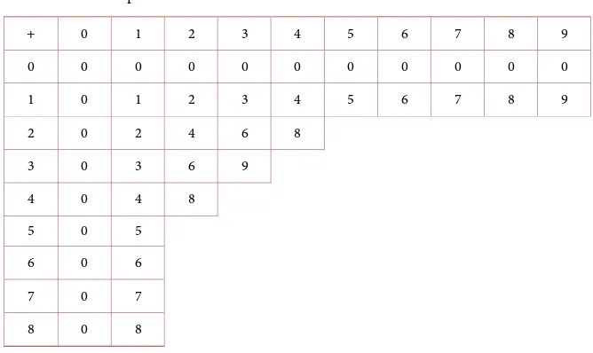
Axiom 2. The addition table. Axiom 3. The multiplication table.
Axiom 1 says that 0 and 1 are the additive and multiplicative identities defined by Table 1 and Table 2.
The rest of the digits are generated by or sums of 1. Thus, 2 = 1 + 1, 3 = 2 + 1, 4 = 3 + 1, 5 = 4 + 1, 6 = 5 + 1, 7 = 8 + 1 and 9 = 8 + 1. The base is 10 = 9 + 1.
DOI: 10.4236/apm.2018.88044 726 Advances in Pure Mathematics
Table 1. The addition table.
+ 0 1 2 3 4 5 6 7 8 9
0 1 2 3 4 5 6 7 8 9
1 2 3 4 5 6 7 8 9
2 3 4 5 6 7 8 9
3 4 5 6 7 8 9
4 5 6 7 8 9
5 6 7 8 9
6 7 8 9
7 8 9
8 9
Table 2. The multiplication table.
+ 0 1 2 3 4 5 6 7 8 9
0 0 0 0 0 0 0 0 0 0 0
1 0 1 2 3 4 5 6 7 8 9
2 0 2 4 6 8
3 0 3 6 9
4 0 4 8
5 0 5
6 0 6
7 0 7
8 0 8
3.2. The Inverses and Terminating Decimals
The additive inverse of an integer x, denoted by −x, satisfies the equation, 0
x+ − =x (4) We write the product of integers a and b as a(b) or ab. The multiplicative in-verse of a nonzero integer x, denoted by 1/x, satisfies,
( )
1 1x x = (5)
provided x does not have a prime factor other than 2 and 5. The quotient of two integers x by y, denoted by x/y satisfies,
x yz= (6) In scientific notation we write an integer N as follows:
1
1 1 10n 110n 1
n n n n
N a a a a a − a
− −
= = + ++ (7)
where the aj’s,
j
=
1,2, ,
n
, are digits. A terminating decimal in the metric [image:7.595.205.539.300.499.2]DOI: 10.4236/apm.2018.88044 727 Advances in Pure Mathematics
( )
( )
( )
1 1 1 1
–1 2
1 1 1 2
2 –1
1 1 1 2
. .
10 10 10 10 10
10 10 0.1 0.1 0.1 ,
n n k k
n n k
n n k
k
n n
n n k
N a a a b b b
a a a b b b
a a a b b b
− − − − = + + + + + + + = + + + + + + + (8)
where a an n–1a1 is the integral part, b b1 2bk the decimal part which is well-defined since 10 has only the factors 2 and 5 and its reciprocal, 1/10 = 0.1, is a terminating decimal. Thus, a terminating decimal is defined.
What happens to x/y if x and y are relatively prime, i.e., they have no common factor? In this case continued division does not yield a terminating decimal and therefore, the quotient is ill-defined. We extend the real number system to in-clude not only the nonterminating decimals but also its closure in a suitable norm that we will introduce later. In R only division by 0 is disallowed. In R* di-vision by a prime other than 2 and 5 yields a nonterminating decimal which is defined but should be disallowed in R.
3.3. Basic Concepts
In scientific notation we write an integer N as follows: 1
1 1 10n 110n 1
n n n n
N a a a a a − a
− −
= = + ++ , (9)
where the aj’s,
j
=
1,2, ,
n
, are digits. A terminating decimal in the metricsys-tem or scientific notation (base 10 place-value numerals) is written as follows:
( )
( )
( )
1 1 1 1
–1 2
1 1 1 2
2 –1
1 1 1 2
. .
10 10 10 10 10
10 10 0.1 0.1 0.1 ,
n n k k
n n k
n n k
k
n n
n n k
N a a a b b b
a a a b b b
a a a b b b
− − − − = + + + + + + + = + + + + + + + (10)
where a an n–1a1 is the integral part, b b1 2bk, the decimal part which is de-fined since 10 has only the factors 2 and 5 and its reciprocal, 1/10 = 0.1, is a ter-minating decimal. Thus, a terter-minating decimal is defined. A decimal is defined if all of its digits are defined or there is an algorithm for finding any digit.
3.4. The Nonterminating Decimals
A sequence of terminating decimals of the form,
1 1 2 1 2
. , . , , . n, ,
N a N a a N a a a (11) where N is an integer, an a digit and there is a rule for choosing each an, is called
standard generating sequence or g-sequence. A nonterminating decimal is the g-limit (g-lim) of its nth g-term,
1 2
. n
N a a a (12) as n ∞, i.e., g-lim
(
N a a. 1 2 an)
=N a a.1 2 an . Note that the g-limit of aDOI: 10.4236/apm.2018.88044 728 Advances in Pure Mathematics 1 2
0
k k k
a = =a+ =a+ = (13)
For the first time (12) defines a nonterminating decimal [5]. The nth g-term of (11) approximates the nonterminating decimal (12) at maximum margin of error of 10−n provided each nth g-term is computable, i.e., there is some
algo-rithm or rule for determining or computing the digits. The scientific calculator has this algorithm for every decimal. The g-limit of (11) is the nonterminating decimal (12) provided the nth digits are not all 0 beyond a value of n. In this case, we say that the g-sequence (11) converges to the nonterminating decimal (12) in the g-norm. Otherwise, it is terminating. A decimal consists of the integral part, the integer left of the decimal point; the decimal part is the se-quence of digits to the right of the decimal point. The integers are ill-defined by the field axioms of the real number system but defined in the constructivist real number system by Axioms 1, 2 and 3 [5] as the integral parts of the decimals.
It would be an appropriate special problem for undergraduate mathematics major to study a class of nonterminating decimals with a given algorithm for computing its digits, e.g., normal decimal. Every digit in a normal decimal is taken at random from the ten digits 0, 1, 2, ···, 9. To stimulate creativity, the stu-dent may think of a certain algorithm and derive the properties of the decimal generated by it. In the real number system the rationals coincide with the termi-nating decimals which are periodic. Since the concept “irrational” is ill-defined there are only two types of real numbers—terminating and nonterminating. The scientific calculator which has the algorithm for approximating all decimals by truncation at desired margin of error. Ramanujan’s continued fraction is equiv-alent to a nonterminating decimal when the denominator has prime factor other than 2 or 5.
We define the nth distance rn between two decimals a, b as the numerical
val-ue of the difference between their nth g-terms, an, bn, i.e., rn = a bn− n , and their g-distance is the g-limit of rn. The nth g-term of a nonterminating decimal
re-peats every preceding g-term so that if finite initial g-terms are deleted the g-terms and g-limit of the remaining g-sequence are unaltered. Thus, a nonter-minating decimal has many g-sequences belonging to the equivalence class of its g-limits.
Approxi-DOI: 10.4236/apm.2018.88044 729 Advances in Pure Mathematics mation makes sense only when what is being approximated is known.
As we raise n in (12), the tail digits of the nth g-term of any decimal recedes to the right indefinitely, i.e., it becomes steadily smaller until it is indistinguishable from the tail digits of the rest of the decimals. Although it tends to 0 in the stan-dard norm it never reaches 0 in the g-norm since the tail digits are never all equal to 0; it is also not a decimal since the digits are not fixed. We refer to it as an algebraic continuum distinct from the topological continuum.
At present the natural numbers are defined as 0; its successor, 1; 2, the suc-cessor of 1; 3, the sucsuc-cessor of 2; etc. There is no axiom defining them. We take a surjection of the natural numbers onto the integers, n
↔
N, N the integral part of a decimal and N =0,1,, which makes them equivalent mathematical spaces since they have exactly the same properties with respect to the binary oper-ations + and × [19]. We define a natural number as the integral part of some de-cimal.The g-norm simplifies computation considerably [5] since the result is ob-tained digit by digit and avoids radicals which are ill-defined.
3.5. The Dark Number
d
*
Consider the iterated product or power,
( )
0.1 ,n n=1,2,; (14)it defines the sequence
0.1,0.01,0.001, (15) This is not a g-sequence since the g-terms do not repeat; we call it d-sequence. Each term moves towards 0 but does not reach 0. The d-sequence defines the d-limit of the d-sequence (15) called the principal d-limit dp because every
d-limit is derivable from it. For each x ∈ R*,
0< <d x (16) Consider the sequence,
( )
0.1 0 1 , 1,2, ; 0,1,2, ,9n
k
a a a n k
−
= =
(17)
where ak is any of the decimals, 0,0.1,0.2,0.3, ,0.9 and a1, , ak decimal digits in the sequence not all 0 simultaneously. For any x ∈ R*, 0 < d < x. There are countably infinite d-sequences and d-limits in (17) all of which share the same properties. The set of g-limits is not empty; we call it the dark number d* so that d* has countably infinite elements each of which satisfies,
*
0<dk <x x, ∈R ,k=1,2, (18) The standard limit of (17) is 0 but its d-limit d* is greater than 0 according to (18). Therefore, they differ by d*. The d-limit has special properties not shared by other elements of R*. In fact, it has a different arithmetic.
If x is a nonzero decimal, terminating or nonterminating, there is no differ-ence between (0.1)n and x(0.1)n, as n ∞, because they become
DOI: 10.4236/apm.2018.88044 730 Advances in Pure Mathematics lim(x/sinx) = 1, as x 0; in the proof, it uses the fact that sinx x< <tanx or 1<xsinx<secx where both extremes tend to 1 so that the middle term tends
to 1 also. In our case, if 0< <x 1, 0<x
( ) ( )
0.1n< 0.1n and both extremes tend to 0; so must the middle term and they become indistinguishably small as n → ∞. The middle term, however, reaches d*. In this sense, computation in R* is more precise.If x > 1, we simply reverse the inequality and obtain the same conclusion. Therefore, we may write, xdp = dp (where dp is the principal element of d*) and
since the elements of d* share this property we may write xd* = d*, meaning, that xd = d for every element d of d*. We consider d* the equivalence class of its elements. In the case of x + (0.1)n and x, we look at the nth g-terms of each and,
as n ∞, x + (0.1)n and x become indistinguishable. Now, since
( )
0.1n >(
( )
0.1m)
n >0 and the extreme terms both tend to 0 as n ∞, so must the middle term tend to 0 so that they become indistinguishably small (the rea-son d* is called dark since it is indistinguishable from 0 but d* > 0).(The dark number d* models the superstring mathematically. The superstring is the fundamental building block of matter. It comprises dark matter, one of the two fundamental states of matter, the other ordinary or visible matter. Dark be-cause it is not detectable. When agitated the superstring becomes a primum, unit of visible matter, e.g., electron, +quark, –quark. They are called basic prima be-cause they comprise every atom [20]).
In R*, the natural norm is the g-norm, i.e., if x ∈ R*, g-norm(x) = x. The nth g-term differs from x by the tail end in the truncation of x at the nth digit. The standard limit of the tail end differs from the g-limit by d*. Every mathematical space has its natural norm that facilitates computation and enhances research.
3.6. Samples of Digital or g-Computation
Approximation makes sense only when we know the number we are approx-imating and the error is bounded above by a desired number.
• Let x = 4.57628… The truncation (Tr) of x at the 3rd g-term is 4.576. The
dis-tance from x or error in the truncation is 0.00028 and d* < 0.00028.
• The standard distance between points x=
(
2.3517 ,5.9372 )
and(
1.1213 ,2.8432)
y= in the plane is approximated by the difference between their truncations at say, the 3rd g-term:
( )
( )
3.094 1.123 1.971Tr y Tr x− = − = (19) • We have no problem with the nth root of a perfect nth power, say, a1/3 where
a = k2, k an integer since it is defined. But how do we compute, say, 37 since 7 is not a perfect square?
Step 1. Divide the interval [0, 10] as follows: [0, 1, 2, 3, 4, 5, 6, 7, 8, 9, 10]. Among the digits, find the largest digit whose cube does not exceed 7. Obviously, it is 1 since 13 < 7 and 23 > 7. Thus, the integral part of 37 is 1.
DOI: 10.4236/apm.2018.88044 731 Advances in Pure Mathematics the largest digit, say, b such that the (1.b)3 does not exceed 7. Clearly, it is 8 since
(1.8)3 = 5.832 < 7 and 9 does not satisfy this inequality. Thus, the closest
trunca-tion of 37 at the first decimal digit is 1.8.
Step 3. To find the next decimal digit divide the interval [0.01, 0.1] as follows: [0.01, 0.02, 0.03, 0.04, 0.04, 0.05, 0.06, 0.07, 0.08, 0.08, 0.1] and find the largest digit, say, b such that (1.8b)3 < 7. In case, it is 5 since (1.85)3 = 6.33 < 7, etc.
We can repeat the calculation to find as many decimal digits as we wish in evaluating 37. The scientific calculator can do this in split second because it has this algorithm for it. The computation avoids radicals which are ill-defined.
For purposes of computation we denote the nth g-term of a decimal by the functional notation n-ξ(x) called n-truncation. Since a g-sequence defines or ge-nerates a decimal we call the latter its g-limit. Since nonterminating decimals cannot be added, subtracted, multiplied or divided, they must be n-truncated first to carry out the operations on them. The margin of error at each step in the computation must be consistent (analogous to the requirement of number of significant figures in physics, the rationale being that the result of computation cannot be more accurate than any of the approximations of the terms). While we can start division by terminating decimal since it starts on the left digits the quo-tient does not exist when the divisor has a prime factor other than 2 or 5.
Let x N a= .1 an and y M b b= .1 n , then
( )
( )
(
)
( )
( )
1 1 - . , - . , - - - , n nn x N a a n y M b b
n x y n x n y
ξ ξ
ξ ξ ξ
= =
+ = +
(20)
(
)
( )
( )
( )
(
( )
)
(
( )
)
(
)
(
( )
)
(
( )
)
- - - , - - - , - - - ,n x y n x n y
n xy n x n y
n x y n x n y
ξ ξ ξ
ξ ξ ξ
ξ ξ ξ
− = −
= =
(21)
provided n-ξ(y) ≠ 0 as divisor. Consider the function f x
(
1, , xk)
of several variables; we n-truncate f as follows:(
)
(
1)
(
( )
1( )
)
- , , k - , , - k .
n
ξ
f x x = f nξ
x nξ
x (22)If f is a composite function of several variables,
(
)
(
)
(
1 1, , t , , s 1, , u)
f g x x g y y then
(
)
(
)
(
)
(
)
( )
(
)
( )
(
)
(
(
( )
)
( )
)
(
1 11 1 1 1)
- , , , , , ,
- - , , - , , - - , , - .
t s u
t s u
n f g x x g y y
f n g n x n x n g n y n y
ξ
ξ ξ ξ ξ ξ ξ
=
(23)
DOI: 10.4236/apm.2018.88044 732 Advances in Pure Mathematics latter.
4. Theorems of R*
The following theorems follow from (5) and (6) of Section 3 and the ensuing discussion.
Theorem. The d-limit of the indefinitely receding to the right nth d-terms of d* coincides with the g-limits of the tail digits of the nonterminating decimals traced by them as the ajs vary along the digits.
Corollary. The tip of the tail end of a decimal is d*.
This means that that we cannot insert a decimal between 0 and d* (the inter-val is full). This is true of every interinter-val of R*, i.e., the whole R* is an algebraic continuum (no gap). A decimal integer has the form N.99…; we shall prove later that they are isomorphic to the integers, i.e., the integral parts of the decimals.
Theorem. If x is an integer, x d+ *=x ; if x is the decimal integer
.99 , 0,1,
N N= then,
( )
(
)
* *
* * *
* * *
*
.99 .99 1 0.99 0.99 1 0.99 1,
; if 0, ;
, 1,2, ;1 0.99 ;
1 .99 1 0.99 .
n
x d N d N N N
x d x x xd d
d d n d
N N d
+ = + = + − = + + − = +
− = ≠ =
= = − =
− − = − =
(24)
The equation x d+ *=x in the theorem says that d* cannot be separated from an integer. Note that x + d* ∈ R*. It also shows that every element of R* has the dark component d*. Recall that the g-closure of R, i.e., its closure in the g-norm, is R*. This is true of the additive inverses, the defined multiplicative in-verses and d*. The reciprocal of d* is u* and the reciprocal of u* is d*. The the upper bounds of divergent sequences of terminating decimals and integers (a sequence is divergent if the nth terms are unbounded as n ∞, e.g., the se-quence 8, 88, …). This unbounded number u* is countably infinite since the countable union of countable sequences is. Like d* it is set-valued. We follow the same convention for u*: whenever we have a statement “u has property P for every element u of u*” we can simply say “u* has property P”. Then u* satisfies these dual properties: for all x,
* *; for 0, * *.
x u+ =u x≠ xu =u (25)
Note the duality of the statements x + d* = x and xd* = d* from Equation (25) and the statements x + u* = u* and xu* = u*. Neither d* nor u* is a decimal; their properties are solely determined by their sequences. Then d* and u* have the following dual or reciprocal properties and relationship:
* * * * * * * *
DOI: 10.4236/apm.2018.88044 733 Advances in Pure Mathematics system and calculus where d* and u* are their counterparts in R*.
The decimals are linearly ordered by the lexicographic ordering “<” defined as follows: two elements of R* are equal if corresponding digits are equal. Let
1 2 1 2
. , .
N a a M b b ∈R (27) Then,
1 2 1 2 1 1 1 1 2
. . if or if , ; if , ; ,
N a a <M b b N M< N M a b= < a b a b= < (28) and, if x is any decimal we have,
* *
0<d < <x u . (29)
The trichotomy axiom follows from the lexicographic ordering of the R* which is linear since there is no gap. This is the natural ordering mathematicians sought among the real numbers but it does not hold in R because there is no li-near ordering of the real numbers since d* is missing. This is what the counte-rexample to the trichotomy axiom [5] says. By inserting d* in these gaps (d* lies between predecessor and successor elements of R) we obtain the closure R*. Then we have the following theorem.
Theorem. The closure of R in the g-norm is R*.
An open problem is whether R can be well-ordered by <. The answer is no since there are gaps in R. However, R* is well-ordered.
4.1. Decimal Integers
Decimal integers are elements of R* form N.99 , N=0,1, 2, is called a
de-cimal integer. We show the isomorphism between the integers and the dede-cimal integers to justify the name in the sense of [19]. However, before doing so we first note that 1 + 0.99… is not defined in R since 0.99… is nonterminating but we can write 0.99= −1 d* so that 1 0.99+ = + −1 1 d*= −2 d*=1.99; we now define 1 0.99+ =1.99 or, in general,
N d
−
*=
(
N
−
1 .99
)
. Twinin-tegers are pairs
(
N N,(
−1 .99)
)
,N=1,2,; the first and second components are isomorphic.Let f be the mapping N→
(
N−1 .99)
and extend it to the mapping d* → 0even if d* is not a decimal; then we show that f is an isomorphism between the integers and decimal integers:
(
) (
)
(
)
(
)
( )
( )
1 .99 1 0.99
1 1 1.99 1 0.99 1 0.99
1 .99 1 .99
f N M N M N M
N M N M
N M f N f M
+ = + − = + − + = − + − + = − + + − + = − + − = + (30)
Thus, addition of decimal integers is the same as addition of integers. Next, we show that multiplication is also an isomorphism.
(
) (
)
(
)
(
)
( )(
)
(
) ( )(
)
(
) ( )(
)
1 .999 1 0.99
1 1 1 0.99
1 1 .99 1 .99 1 0.99
1 0.99 1 0.99
0.99 1 0.99 0.99
f NM NM NM
NM N M N M
NM N M N M
NM N M N
DOI: 10.4236/apm.2018.88044 734 Advances in Pure Mathematics
(
)(
) (
)(
) (
)(
) (
)
(
)
(
)
(
(
)
)
(
)
(
)
(
)
(
(
)
)
( )
(
)
(
( )
)
21 1 1 0.99 1 0.99 0.99
1 0.99 1 0.99
1 .99 1 .99
N M N M
N M
N M
f N f M
= − − + − + − + = − + − + = − − =
We include in the isomorphism the map d* → 0, so that its kernel is the set {d*, 1} from which follows,
( )
d* n=d*and 0.99(
)
n=0.99 ,n=1,2, (32)
If 0 < x < 1, there is no difference between C and x(0.1)n since (0.1)n tend to d*
in the g-norm; it follows that x(d*) = d*. Intuitively, this means that as the d- and g-terms of x(0.1)n and x(0.1)n move to the right towards 0 indefinitely they
become indistinguishable from each other but remain greater than zero. Theorem. Let x = N.99…; then
( )
(
)
* * * * *
* * *
, 1, ; if 0,
, 1,2, , 1 0.99 ; 1 .99 1.99
n
x d x x d N x d x x xd d
d d n d N N
+ = + = + − = ≠ =
= = − = − − = (33)
Note that among the nonterminating decimals, d* and 0.99… serve as the ad-ditive and multiplicative identities, respectively. This means that R* has two multiplicative identity elements, namely, 1 and 0.99… We exhibit other proper-ties of 0.99…. Let K be an integer, M.99… and N.99… decimal integers. Then
(
)
(
)
(
)
(
)
(
)
.99 .99 ,
.99 0.99 0.99 ,
.99 .99 1 .99 .
K M K M
K M K M KM K
M N M N
+ = + = + = + + = + + (34)
To verify that 2(0.999...) = 1.99…, we note that (1.99…)/2 = 0.99…
(
)(
) (
)(
)
(
)
(
) (
)
(
)
(
)
(
)
(
)
(
)
2.99 .99 0.99 0.99
0.99 0.99 0.99
1 .999 1 .99 0.99
2 .99 0.99
1 .99 1 .99
M N M N
MN M N
MN M N
MN M N
MN M N MN M N
= + + = + + + = + − + − + = + + − + = + + − = + + − (35)
(
)
0.99+0.99=2 0.99 =1.99 (36)
4.2. Adjacent Decimals and Recurring 9s
Two decimals are adjacent if they differ by d*. Predecessor-successor pairs and twin integers are adjacent. In particular, 74.5700… and 74.5699… are adjacent. Since the decimals have the form N a a.1 2 an, ,N=0,1,2,, the digits are identifiable and, in fact, countably infinite and linearly ordered by the lexico-graphic ordering. Therefore, they are discrete or digital and the adjacent pairs are also countably infinite. However, since their tail digits form a continuum, R* is a continuum with the decimals its countably infinite discrete subspace.
DOI: 10.4236/apm.2018.88044 735 Advances in Pure Mathematics example, 4.3299… and 299.99… are recurring 9s; so are the decimal integers. (In an isomorphism between two algebraic systems, their operations are interchan-geable, i.e., they have the same algebraic structure and differ only in notation).
The recurring 9s have interesting properties. For instance,
(
1 .99
)
*N
−
N
−
=
d
; such pairs are adjacent because there is no decimal be-tween them. In the lexicographic ordering the smaller of the pair of adjacent de-cimals is the predecessor and the larger the successor. The average between them is the predecessor. Thus, the average between 1 and 0.99… is 0.99… since (1.99…)/2 = 0.99…; this is true of any recurring 9, say, 34.5799… whose succes-sor is 34.5800… Conversely, the g-limit of the iterated or successive averages between a fixed decimal and another decimal of the same integral part is the predecessor of the former.Since adjacent decimals differ by d* and there is no decimal between them, i.e., we cannot split d* into nonempty disjoint sets, we have another proof that d* is a continuum. This is equivalent to the topological continuum. The counte-rexample to the trichotomy axiom debunks the idea that a terminating can be expressed as the limit of sequence of rationals since the closest it can get to it is some rational interval containing rationals whose relationship to it is unknown. The g-sequence of a nonterminating decimal reaches its g-limit, digit by digit. This is one of the advantages of computation in the g-norm. Moreover, a non-terminating decimal is an infinite series of its digits:
1 2 1 2
. n 0. 0.0 0.00 0 n ; 0.99
N a a a =N+ a + a + + a + (37)
5. R* and Its Subspaces
We add the following results to the information we now have about the various subspaces of R* to provide a full picture of the structure R*. The next theorem is a definitive result about the continuum R*.
Theorem. In the lexicographic ordering R* consists of adjacent predeces-sor-successor pairs (each joined by d*); hence, the g-closure R* of R is a conti-nuum.
Proof. For each N N, =0,1,, consider the set of decimals with integral part
N. Take any decimal in the set, say, N a a.1 2, and another decimal in it. With-out loss of generality, let N a a.1 2 be fixed and let it be the larger decimal. We take the average of the nth g-terms of N a a.1 2 and the second decimal; then take the average of the nth g-terms of this average and N a a.1 2; continue. We obtain the d-sequence with nth d-term,
( )
0.5 1 2n
n k
a a a
−
+
, which is a d-sequence of d*. Therefore, the g-limit of this sequence of averages is the pre-decessor of N a a.1 2 and we have proved that this g-limit and N a a.1 2 are predecessor-successor pair, differ by d* and forms a continuum. Since the choice of N a a. 1 2 is arbitrary then by taking the union of these predecessor-successor pairs of decimals in R* (each joined by the continuum d*) for all integral parts N, N=0,1,, we establish that R* is a continuum.
DOI: 10.4236/apm.2018.88044 736 Advances in Pure Mathematics there is a scheme for labeling them by integers and the integers are discrete and countably infinite. We can imagine them as forming a right triangle with one edge horizontal and the vertical one extending without bounds. The integral parts are lined up on the vertical edge and joined together by their branching di-gits between the hypotenuse and the horizontal that extend to d* which is adja-cent to 0 (i.e., differs from 0 by a dark number) at the vertex of the horizontal edge.
Corollary. R* is non-Archimedean but Hausdorff in both the standard and the g-norm and the subspace R of decimals is countably infinite, hence, discrete but Archimedean and Hausdorff. Clearly, R or the set of decimals is a subspace of the constructivist real number system R*.
The following theorem is true in R (standard norm). Therefore, we do not bring in d* in the proof so that this is really a theorem about the decimals in the standard norm but not so in the g-norm where the decimals merge into a conti-nuum at their tail digits and cannot be separated.
Theorem. Every real number is isolated from the rest [20].
Proof. Let p ∈ R be a nonterminating decimal and {qn} a sequence of rationals converging to p from the left. Let dn be the distance from qn to p and take an
open ball of radius dn/10n, with center at qn. Note that qn tends to p but distinct
from it for any n. Take an open ball of radius dn/10n, centered at p and take the
union of open balls, centered at qn, as n ∞ and call it U. If r is any decimal to
the left of p, then r is separated from p by at least d* which is isolated from the rest of the real numbers. The same result holds for any r distinct from and to the right of p.
Here is another surprise that contradicts a theorem in the real number system. Theorem. The rationals and nonterminating decimals are separated, i.e., they are not dense in their union (the first indication of discreteness of the decimals
[21]).
Proof. Let p ∈ R* be a nonterminating decimal, and let q nn, =1,2, be a sequence of rationals towards and left of p, i.e., n > m implies qn > qm; let rn be
the distance from qn to p and take an open ball of radius rn/10n, center at qn.
Note that qn tends to p but distinct from it for any n. Let U=
Un, as n ∞, then U is open and if q is any real number, rational or nonterminating to the left of p then q is separated from p by disjoint open balls, one in U, center at q and the other in the complement of U, center at p. Since the rationals are countable union of open sets U for all the rationals, the nonterminating decimal p is sepa-rated from all the rationals.We use the same argument if p were rational and since the reals has countable basis we take qn a nonterminating decimal, for each n, at center of open ball of
radius dn/10n. Take U to be the union of such open balls. Using the same
argu-ment, a real number in U, rational or nonterminating, is separated by disjoint open balls centered at p.
DOI: 10.4236/apm.2018.88044 737 Advances in Pure Mathematics from the nonterminating decimals and from each other. Clearly, the last two theorems do not hold in R*. We state a theorem that is true in R*.
Theorem. The largest and smallest elements of the open interval (0,1) are 0.99… and d*, respectively [21].
Proof. Let Cn be the nth term of the g-sequence of 0.99… For each n, let In be
open segment (segment that excludes its endpoints) of radius 10−2n centered at
Cn. Since Cn lies in In for each n, Cn lies in (0,1) as n increases indefinitely.
Therefore, the decimal 0.99… lies in the open interval (0,1) and never reaches 1. To prove that 0.99… is the largest decimal in the open interval (0,1) let x be any point in (0,1). Then x is less than 1. Since Cn is strictly increasing n can be
cho-sen so that x is less than Cn and this is so for all subsequent values of n.
There-fore, x is less than 0.99… and since x is any decimal in the open interval (0,1) then 0.99… is, indeed, the largest decimal in the interval and is itself less than 1.
To prove that 1 − 0.99… is the smallest element of R, we note that the g-sequence of 1 − 0.99… is steadily decreasing. Let Kn be the nth term of its
g-sequence. For each n, let Bn be an open interval with radius 10−2n centered at
kn. Then Kn lies in Bn for each n and all the Bns lie in the open set in (0,1). If y is
any point of (0,1), then y is greater than 0 and since the generating sequence 1 − 0.99… is steadily decreasing n can be chosen large enough such that y > Kn and
this is so for all subsequent values of n. Therefore, y > 1 − 0.99… and since the choice of y is arbitrary, 1 − 0.99… is the smallest number in the open interval (0,1) greater than 0.
This is not true in R* since 1 − 0.99… and 0.99… are not defined. Most text-book in college algebra have these errors.
Goldbach’s Conjecture. An even number greater than 2 is the sum of two primes.
The original proof of this 250-year-old conjecture is in [20] but we reproduce it here for completeness. Like Fermat’s equation the conjecture is indeterminate and need not have a solution in R. It has, however, solutions in R*.
We note first that an integer is a prime if it leaves a positive remainder when divided by another integer other than 1. We retain this definition of a prime in R* but the remainder is d* which is not a real number.
Proof. The conjecture is not vacuous since it is true when p = q = 2. In fact, it is true when n < 10. Let n be an even number greater than 10. Then there is some prime number p greater than 3 and another number q such that p + q = n. If q is prime then the theorem is proved; otherwise, it must be divisible by some integer (0 remainder) other than 1 and q. Then we add to q the dark number d* > 0 and we have q + d* = q and division of q by any nonzero integer yields nonzero remainder d*, i.e., q is prime.
It follows from the proof that every element of R* greater than 3 is a prime. In R with all its defects, every real number is composite since if x ∈ R, x= x x,
where x is some decimal. In this sense R and R* are dual. For example,
( )( )
DOI: 10.4236/apm.2018.88044 738 Advances in Pure Mathematics can be approximated only when the number under the operator 4 is not a perfect fourth power.
5.1. The Structure of R*
We now have a sense of how the decimals are arranged by the lexicographic or-dering. Below is a sequence of successor-predecessor pairs at the boundaries of a rational and nonterminating decimals.
.4999100 .4998999 .4999999 .499999899
N N N N
(38)
The ellipses after the first and second rows are filled with d* alone. The el-lipses between the third and fourth rows are filled with d* and nonterminating decimals. The largest decimal in the open interval (N.49100, N.49999899…) is the decimal integer N.49100… and the smallest is the nonterminating decimal N.49999899… Starting from the bottom going up, the decimals with integral part N are arranged as predecessor-successor pairs each joined by d*. Each gap (represented by ellipses) is filled by countably infinite adjacent predeces-sor-successor pairs also joined by d* so that their union is a continuum. Clearly, R* is linearly ordered by <, the lexicographic ordering; d* joins every decimal to its successor and d* cannot be split from either.
5.2. Resolution of a Paradox and Other Important Results
Every convergent sequence has a g-subsequence defining a decimal adjacent to its standard limit [5].
If a decimal is terminating it is the standard limit itself. We express this as a theorem:
Theorem. The difference between the standard limit and the g-limit is d*. (2) It follows from (1) that the standard limit of a sequence of terminating de-cimals can be found by evaluating the g-limit of its g-subsequence which is ad-jacent to it. This is an alternative way of computing the limit of ordinary se-quence.
(3) In [22] several counterexamples to the generalized Jourdan curve theorem for n-sphere are shown where a continuous curve has points in both the interior and exterior of the n-sphere, n=2,3,, without crossing the n-sphere. Our
ex-planation is: the functions cross the n-sphere at dark numbers.
(4) Given two decimals and their g-sequences and respective nth g-terms An,
DOI: 10.4236/apm.2018.88044 739 Advances in Pure Mathematics evaluated digit by digit in terms of their components without the need for eva-luating roots. In fact, any computation in the g-norm yields the results directly, digit by digit, without the need for intermediate computation such as evaluation of roots in standard computation. (The decimals are “glued” together by d* to form the continuum R*)
(5) We know from [1] that the celebrated Banach-Tarski paradox is vacuous, does not exist.
(6) Well-ordering Theorem. Every sequence R* bounded below has a great-est lower bound and every sequence in R* bounded above has a least upper bound (the bound in either case is a decimal, terminating or nonterminating).
Proof. If the sequence has a lower bound it has standard limit S. Then S + d* = S is the greatest lower bound because any number to the right of S will not be a lower bound. The proof is similar for the least upper bound.
The proof of this theorem in R is flawed because it uses a variant of the axiom of choice. It also involves vacuous concepts.
(7) If the standard limit of a sequence of decimals exists then it is constructible since it is adjacent to the g-limit of some g-sequence.
We have clearly identified the ambiguous concepts of R, defined some of them in R* and discarded some that cannot be fixed, e.g., the irrationals. We have also identified certain theorems in R that are false in R*. All theorems in real analysis that relies on the axiom of choice are not true, e.g. the Heine-Borel theorem and the existence of non-measurable set [13].
5.3. Advantages of the G-Norm
• Avoids indeterminate forms.
• In computation, the g-norm yields the answer directly, digit by digit, and avoids intermediate computation.
• Since the standard limit is adjacent to the g-limit of some g-sequence, eva-luating it reduces to finding some nonterminating decimal adjacent to it. A decimal is approximated by the appropriate nth g-term (n-truncation). • Calculation of distance between two decimals with the g-norm is direct, digit
by digit, and involves no root.
• In computation, taking root of a prime is avoided by using n-truncation; the error < 10−n.
• The g-norm is the natural norm for R*. It simplifies computation and pro-vides the best approximation.
• Most of all, while the standard norm brings in the nonexistent radicals the g-norm does not. Thus, the g-norm is the natural norm for R*.
cal-DOI: 10.4236/apm.2018.88044 740 Advances in Pure Mathematics culator has the algorithm for computing the g-sequence of a decimal and, natu-rally, the g-limit as well. This is true of the computer. The algorithm defines an exponential function directly and without a flaw. Extension to fractional expo-nent is easy since the calculator approximates the g-limits of roots.
We conclude this section with the resolution of Fermat’s last theorem.
6. The Counterexamples to FLT
Given the contradiction in negative statement, we use Fermat’s equation in place of Fermat’s last theorem; its solutions are counterexamples to FLT. We sum-marize the properties of the digit 9.
1) A finite string of 9 s differs from its nearest power of 10 by 1, e.g., 100
10 −99 9 1 = .
2) If N is an integer, then
(
0.99)
N =0.99 and, naturally, both sides of this equation have the same g-sequence. Therefore, for any integer N,(
)
(
0.9910)
N =(
9.99)
10N.3)
( )
d* N =d*; 0.99(
(
)
10)
N +d*=10 ,N N=1,2,Then the exact solutions of Fermat’s equation are given by the triples
(
x y z, ,) (
=(
0.99)
10 , ,10T d* T)
, T =1,2,, that clearly satisfies Fermat’s equ-ation,n n n
x +y =z , (39)
for n = NT > 2. Moreover, for k=1,2,, the triples (kx, ky, kz) also satisfy
Fermat’s equation. They are the countably infinite counterexamples to FLT that prove the conjecture false. This is the original resolution of FLT in [18]. (One counterexample is, of course, sufficient to disprove the conjecture)
7. Transcendental Functions
Algebraic functions are defined only when their domains are terminating de-cimals. Those that are undefined we include them under transcendental func-tions where the argument ranges through R*. There are special funcfunc-tions which do not presently belong to the class of transcendental functions. They will be treated in a sequel part of under the mathematics of the grand unified theory
[23].
If y = f(x) is a transcendental function we define f x
( )
=g-lim(
f s( )
)
as s → x. The limiting process is taken along a g-sequence. There are, of course, func-tions which do not have g-sequences. They are special funcfunc-tions which require a different treatment. This will be discussed in a different paper. Consider the ex-ponential function.Let x N x x= .1 2, then ex =eN x x.1 2; if we replace x by y = f(x) then,
( ) g-lim( ( ))
ef x =e f s as s → x. (40) It follows from (2) that
( )
(
( )
)
e e
log f x =log g-limf s , as s → x. (41)
DOI: 10.4236/apm.2018.88044 741 Advances in Pure Mathematics
( ) g-lim( ( ))
10f x =10 f s as s → x. (42) Let logf(x) be a logarithmic function base 10. Then we have this definition:
( )
(
( )
)
logf x =log g-limf s , as s → x. (43)
Equations (2)-(5) define the exponential and logarithmic functions for the first time (without flaw). They are inverse functions of each other. The circular functions and their inverses are treated in the same way.
Since the exponential and logarithmic functions base e are convertible to ex-ponential and logarithmic functions base 10, we have now defined transcenden-tal functions.
We can approximate sums and products of these functions at a given point by suitable truncations. For example:
• To compute ex at x = a, we calculate the g-limit(f(x)), as x → a; ex is
approx-imated by suitable truncation.
• To evaluate π up to the 5th decimal digit, we use the infinite series expansion
of π which is π = 3.14159… Then we truncate it at the 5th digit and the error
will be less than (0.1)5. The standard decimal expansion of π is the closest
approximation of its g-limit and differs from the g-limit by d*. Of course, the scientific calculator can calculate π quickly by its algorithm.
• We illustrate the algorithm for calculating the nth root of a decimal using 3.
Step 1. The largest integer n such that such that n2 < 3 is 1. Therefore, the
integral part of 3 is 1.
Step 2. Divide the interval [0,1] into subintervals at the following points: 0, 0.1, 0.2, 0.3, 0.4, 0.5, 0.5, 0.6, 0.7, 0.8, 0.9, 1. The largest division point n such that (1.n)2 < 3 is n = 0.7. Therefore, the truncation of 3 at the first decimal digit is
1.7.
We continue the calculation and find that 3=1.732050808. This is ex-actly how the scientific calculator computes nth roots. Then calculation with fractional exponents, terminating or nonterminating, is known. The only re-quirements for valid approximation is: what is being approximated is known and the error is bounded away from 0 by d*.
Theorem. The decimals are ordered by the lexicographic ordering in R* and the trichotomy axiom is true in R* and follows from the lexicographic ordering.
Proof. The closure of R in the g-norm which is R* fills in the gaps in R with d* that allows the linear ordering of R* by the lexicographic ordering.
Theorem. Let K be an integer, M.99··· and N.99··· decimal integers. Then
(
)
.99 0.99 .99
K M+ =K M+ + = K M+ ,
(
.99)
(
0.99)
(
0.99)
K M =K M+ =KM K+ =KM K+ (since K
(
0.99)
=K),(
)
.99 .99 1 .99
predeces-DOI: 10.4236/apm.2018.88044 742 Advances in Pure Mathematics sor-successor pairs (each joined by d*); therefore, the g-closure R* of R is a con-tinuum.
Corollary. The average between the predecessor and its successor is the suc-cessor.
Corollary. R* is non-Archimedean but Hausdorff in both the standard and the g-norm and the subspace R of decimals is countably infinite, hence, discrete but Archimedean and Hausdorff.
Theorem. R* is a continuous linear array of predecessor-successor pairs with d* inserted between them.
8. The Complex Vector Plane
The complex vector plane C* is the rectification of the complex number system C. It the circular functions as a subspace.
8.1. The Element j as Operator on Plane Vectors
The rectification of C involves the replacement of the vacuous concept i by the left-right plane vector operator j, rotation of the clockwise or positive rotation (x,0) about the origin by π/2. Then the coordinate axes are generated by applying j on the x-axis, i.e., j(x,0) = jy (rotation of the x-axis by π/2), applying j on the jy-axis, i.e., jj(y,0) = (−x,0) (rotation of the −x-axis by π/2) to obtain the negative x-axis, and j on the –x-axis, i.e., jjj(−x,0) = j(−y,0) (rotation of the negative x-axis by π/2) to obtain the −y-axis and applying j on the negative y-axis, i.e. jjjj(−x,0) = (x,0) (rotation of the negative y-axis by π/2) to obtain the x-axis. Thus, we have the cyclic values of the composites of j with itself:
( )
= ,( )
= 2( )
= − , 2( )
= − 3( )
= − , 3( )
= 4( )
= .j 1 j jj 1 j 1 j jj 1 j 1 j jj 1 j 1 1 (45)
The complex vector plane is generated by applying j on (x,0) through θ, 0 ≤ θ ≤ 2π. We define the operator −j as inverse operator of j, i.e., when applied on a vector v we rotate it clockwise by π/2 so that −j(1) = j(−1). Applying composite mappings on the unit vector 1 along the x-axis successively, we have the four cyclic images of 1 in (1) in reverse order. For n > 4, the cycle is repeated and we obtain jn = j(jn−1), n = 1, 2, ···, where we define j0= 1.
8.2. Scalar and Vector Operations
For completeness, we introduce scalar multiplication. If α is an element of R* (scalar), αj is a vector of modulus α along the y-axis. Note that scalar multiplica-tion commutes with j. If β is another scalar,
( )
αβ j j=( ) ( )
αβ = jα β β α=( ) (
j = βα)
j, (46) which follows from j being left-right operator and the commutativity of multip-lication in R*. From commutativity and associativity of multipmultip-lication we have, for α, β, γ ∈ R*,DOI: 10.4236/apm.2018.88044 743 Advances in Pure Mathematics Also, from distributivity of multiplication in R* with respect to addition we have,
(
) (
) ( ) ( )
α β γ+ j= αβ αγ+ j= αβ j+ αγ j. (48)
Thus, we have retrieved the basic properties of the complex plane. We call j the complex vector operator. Every vector in the complex vector number system has new real and complex components; conversely, a vector is the vector sum of its new real and complex components. Thus, a vector z in it has standard form,
(
)
*or , , ,
α β α β α β
= + = ∈
z j z j R . (49)
The arithmetic of the complex plane holds provided that whenever 1 appears as a factor we interpret it as a unitary vector operator so that 1α = α, the vector of modulus 1 along the x-axis. Thus, we retain in the complex vector plane and the vector algebra of the complex plane, the latter isomorphic to the former. All concepts of the complex plane except i which is replaced by j carry over to the complex vector plane. For example, the norm or modulus of the complex vector v = α + βj, denoted by |v|, is given by,
(
2 2)
1 2 α β= +
v , (50)
the square root of the product of z and its conjugate, α− βj. The dot product of vectors u and v is given by
cos ifθ , , 0 if or
⋅ = ≠ ≠ ⋅ = = =
u v u v u 0 v 0 u v u 0 v 0, (51)
where θ ∈ R*.
Two parallel vectors with the same norm are equivalent. Therefore, a vector can be translated to a standard vector with initial point at the origin.
The vector additive and multiplicative identities are the vectors 0 and 1, re-spectively, where the latter called the unit vector coincides with its real compo-nent 1. The scalars are subject to the operations in R* and scalar multiplication on vectors which are both commutative and associative. With the complex vec-tor arithmetic now defined we have verified that the operavec-tor j applies to any vector in the complex vector plane. Applying j on the vector z of (5), we have,
( ) (
= α+ β)
= − +β αj z j j j , (52)
a positive rotation of vector z by π/2.
8.3. The Operator h
θWe introduce the more general complex left-right operator hθ on the complex
vector plane appropriate for analytical work:
(
a b)
eθ(
cos sin)
θ + = j = θ+ θ
h j r r j , (53)
where a, b ∈ R*, r is the radius vector of rejθ represented by an arrow with initial