A Variational Approach for Numerically Solving the
Two-Component Radial Dirac Equation for One-Particle
Systems
Antonio L. A. Fonseca1, Daniel L. Nascimento1, Fabio F. Monteiro2, Marco A. Amato1
1
Institute of Physics and International Center for Condensed Matter, University of Brasília, Brasília, Brazil
2
Faculdade UnB Planaltina, University of Brasília, Brasília, Brazil Email: [email protected]
Received February 1,2012; revised March 9, 2012; accepted March 20, 2012
ABSTRACT
In this paper we propose a numerical approach to solve the relativistic Dirac equation suitable for computational calcu- lations of one-electron systems. A variational procedure is carried out similar to the well-known Hylleraas computa- tional method. An application of the method to hydrogen isoelectronic atoms is presented, showing its consistency and high accuracy, relative to the exact analytical eigenvalues.
Keywords: One-Electron Systems; 2D Dirac Equation; No-Inertial Frames; Variational Approach
1. Introduction
The study of hydrogen-like models plays an important role to test new approaches, and also in the description of the electronic structure of atomic and molecular systems. In this context, relativistic effects are of the most impor- tance in a complete description of the physical system, mainly as the atomic mass of elements increases. Indeed, these effects play a crucial role in the description of the electronic structure of heavy elements.
Nevertheless, numerical methods used to take into ac- count relativistic effects face several setbacks when the Dirac equation is used due to the existence of a negative continuum energy spectrum associated to the Dirac Hamil- tonian operator, e.g., the appearance of instabilities in numerical calculations. Such methodologies are based on straight minimization of the expected values of the Dirac Hamiltonian with respect to a subset of the possible Dirac spinors [1-8]. As it is well known, it is very diffi- cult to describe systems of many-electron atoms and mole- cules using the relativistic quantum mechanics approach. Even, in the Dirac’s relativistic framework, where a one- electron spinorial solution is a two-vector whose com- ponents are scalar wave functions, the description is in- complete. Hence, a full relativistic description of the atomic and molecular electronic structure demands the application of Quantum Electrodynamics methods and consequently, the difficulty of implementing computational treatment for many-electron system increases. A survey of the cur- rently available analytical solutions for relativistic one electron atoms may be found in Maple or Mathematica
codes in [9,10] which may be valuable in comparing re- sults of different theories.
from the literature, our method to obtain the energy val- ues of the Dirac-Coulomb problem derives directly from the Dirac equation and not from the usual minimization procedures of the Dirac Hamiltonian. In this context the results presented in the paper are new. Although the theoretical aspects have been discussed [12] in order to make the paper more self-contained, we devote Section 2 to a short review of the mathematical tools of that refer- ence. In Section 3 we develop the numerical methods and apply them to hydrogen isoelectronic atoms showing its consistency and high accuracy, relative to the exact ana- lytical eigenvalues. The conclusions are summarized in Section 4.
2. An Irreducible 2D Form for the Dirac
Equation
The Dirac wave equation [13] is naturally associated with complex manifolds of the form , with
. The usual 4D representation demands that
n n
C C
1
n n2
because the electron spin is introduced as an implicit or algebraic degree of freedom, which implies the need of four linearly independent matrices to construct the standard 4-spinor Dirac equation. However, we will show here that an irreducible 2D representation is also possible in for a hydrogen-like problem. In fu- ture we expect generalize the procedure for many elec- tron problems, by considering other sets.
4 4
CC
n
C
n
C
Since objects of C , that is the SU2 group are complex quadratic matrices, [14] the corresponding wave function must be a two-spinor of the form
C
2 2
1 2
, so that we consider the stationary Hamiltonian problem
1, 2
E
1, 2
,H
,
x y z
(2.1)
with
y x
H i i m (2.2)
with is
.z y x x y
being the usual Pauli matrices. In order to investigate what angular momentum corresponds to a constant of motion in this model we consider the z com-ponent of the angular moment vector
J i (2.3)
Equation (2.3) can easily be verified that do not com- mute with the Hamiltonian H
H J, z
x x yy. (2.4) However, we should observe that
H J, z
2
x x y y
, (2.5) so that the effective operator,1 , 2
z z
M J (2.6)
commutes with H and therefore is a constant of motion. In this context, M and H may be simultaneously diago- nalized, that is
1, 2
1, 2
,M j
j
(2.7)
where is an eigenvalue of M.
In order to check if our irreducible Dirac equation generates the correct one particle solution, we consider a Coulomb potential
r Z r , where Z is the nuclear charge and 1 137 is the fine structure con-stant and determines the energy levels for hydrogenic atoms.Equation (2.1) is explicitly written as a two component Dirac-like linear systems of equations
1 1 2 0
x i y q
2 2 1 0
x i y q
(2.8a)
and
, (2.8b)
where we have introduced q m
EZ r
r, In ordinary polar coordinates
.
, the differential operators in Equations (2.7) and (2.8) become
1
,
i
x i y e r ir
Jz i . (2.9)
By substituting Equation (2.9) into Equation (2.7) and Equations (2.8), it is straightforward to verify that the general solutions are
1
1 02 2
1 , 1 , 1 2
n
i j r s
r e R r R r r e
a r
(2.10a)
1
1 02 2
2 , 2 , 2 2 1
n
i j r s
r e R r R r r e
ar(2.10b)
The exact solution has recursion relations given by
1
22 2 2
1 2
2 1
1 2 1
n j s j Z
a a
s s j Z
(2.11a)
2 12 1 2
1 2
j s Z
a a
s j Z
, (2.11b)
2 2 2
s j Z
where , a01 , 0 n0 n j
with 1 j n 1, 2,
The remaining parameters are
given by 2 2 1 2
m E
1 and 2 m E . Finally,
Equations (2.11) form a polynomial solution of finite de- gree for Equations (2.7) and (2.8), if and only if, the cor- responding energy eigenvalues are given exactly by
1 2 2 2
, 2
2 2 2
2 2 2 2
2 2 1 3 1 1 4 2 n j Z E m
n j j Z
Z Z n
m j n n
(2.13)
The first two radial functions and for the hydrogen ground state are
1n j, ( )
R r R2 n j, ( )r
1
2 1
1 1,1
r
R r e , (2.14a)
,1 1 1,1
2 Z R R
R
n j
2
2 1 . (2.14b)
We would like to point out that the proportionality between 2 n j, (the so called small component) and
1n j, (the so called large component) observed in
Equation (2.14) occurs only when ; otherwise these functions are linearly independent.
R
3. Numerical Hylleraas-Like Variational
Problem
We have seen in [12] that the method is analytically suc- cessful for one-electron atoms. We now formulate a nu- merical version, which is based in a Hylleraas-like varia- tional approach given in [15], and aims to be extended to two or more electron systems in a future work. This time, instead of solving analytically the system composed of Equations (2.8), we isolate
1 1
x i y
q
2
, (3.1)
and substitute into Equation (2.8b), obtaining
1 11 0 y
q
x i y x i
q
(3.2)
We now express Equations (2.8) by means of an ex-tremum problem in which the space integral of a general Lagrangean density
,
x y,
,
, , ,L x y x y
is sta- tionary against small algebraic variations in the form of
x y
1 ,about the form of the exact eigenfunctions
x y
and
02 n
r s
e a r
d d 0 L x y
1 1
2 2
1 , 1 , 1
i j
r e R r R r r
(3.3)
given by
, (3.4) which leads to the corresponding differential equation obeyed by the Lagrangean:
L 0, x y x y L L
(3.5)
where is the complex conjugate of that satisfies the asymptotic condition lim 0
r .
By comparing Equation (3.3) with Equation (3.5), it is clear that the only possible Lagrangean should be
For 1, we recover Equation (2.10a) or, making
use of Equation (2.9) one obtains Equations (2.8). Now we construct a variation function by a product of a power series and undetermined coefficients times the exact so- lution in Equation (2.10b)
,
y
L q
x i y x i
q
(3.6)
1
21 1 1
0
, ,
N i j
r e R r R r R r c r
(3.7) cwhere N is an integer and to be specified later.
The variation process implied in Equation (3.4) is then performed directly, by requiring the vanishing of the par- tial derivatives of the integral of L with respect to the undetermined power series coefficients , whose val- ues produce the algebraic variation of the form of
x y,
1 ,about the form of the exact eigenfunction x y , i.e.,
0 0 0,1,2,
d d 0 d d 0.
L x y L x y
c
(3.8)More explicitly, after substituting Equation (3.7) into Equation (3.6), the modified Lagrangean becomes
2 1 2 1 2 1 1 d 1 . d j R
L R q R
q r r
, (3.9) xBecause the function 1 y
E E m is not in general an ei-genfunction of the Hamiltonian operator, Equation (3.7) does not lead naturally to a finite system of equations, as can be seen in Equation (2.8). Then it is necessary to truncate the power series of the modified function at same order of precision given by the integer N. In fact, Equation (3.7) leads us to an infinite system of linear equations such that the determinant must vanish in order to have a non trivial solution, so it has to be truncated, as usual in Hylleraas-like calculations, at a given order of precision [15]. The whole computational process is so simple that we could express and run the corresponding numerical algorithm using only what is available in Ma- ple algebraic software.
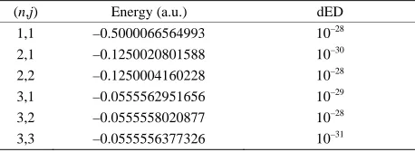
The numerical results of energies n j, n j, in
[image:3.595.309.538.652.736.2]atomic units are calculated for the ground state and sev- eral excited states of hydrogen atom and are given in
Table 1, in which dED stands for the numerical deviation with respect to the exact analytical values given in Equa- tion (2.13). To obtain these results we have used N = 5 in Equation (3.7) and 4 iterations. Table 2 shows the set of
Table 1. Relativistic energy of the ground and excited states for several n and j quantum numbers of atomic hydrogen.
(n,j) Energy (a.u.) dED 1,1 –0.5000066564993 10–28
2,1 –0.1250020801588 10–30
2,2 –0.1250004160228 10–28
3,1 –0.0555562951656 10–29
3,2 –0.0555558020877 10–28
Table 2.Set of fine structures with quantum number n = 10 for atomic hydrogen.
j Energy (a.u.) dED
1 –0.0050000246288 10–33
2 –0.0050000113158 10–33
3 –0.0050000068782 10–34
4 –0.0050000046594 10–34
5 –0.0050000033281 10–34
6 –0.0050000024406 10–35
7 –0.0050000018067 10–35
8 –0.0050000013312 10–36
9 –0.0050000009614 10–36
10 –0.0050000006656 10–37
fine structure levels for the quantum numbers1 1
of the hydrogen atom, where we have used N = 7 and the order of precision dED was obtained after 4 iterations.
0
j n
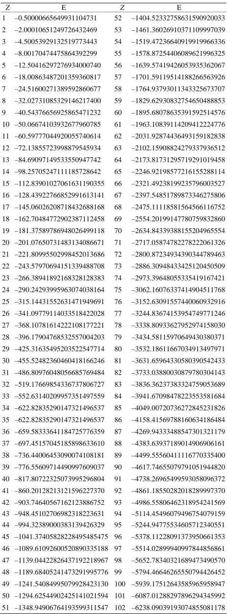
The energy levels for several hydrogen isoelectronic atoms calculated by the present theory are shown in Ta- ble 3. In this table ni is the number of iterations for a given
order of precision, N is the truncation integer of the power series in Equation (3.7) and dED gives the comparative accuracy between the exact analytical Dirac solution and our numerical results. Using N = 9 to calculate the energy of Ba+55 we have obtained a precision of 10–14 against 10–31 for N = 11. In the case of U+91 we have obtained the precision of 10–9, 10–23 and 10–31 for N = 9, N = 11 and N
= 15, respectively. In order to improve precision, we only have to increase the value of N in the series in Equation (3.7). We can also observe in Table3 that when Z in- creases, the interaction is slower and it is necessary to increase N as well. In Table 4 we compare the results obtained by our approach with the results found in the literature. The order of precision of our results (dED), in
Table 4, is 10–30. The numerical applications shown in
Tables 1-4 indicates that our method has a high numeri- cal accuracy with respect to the analytical results ob- tained by Dirac.
4. Conclusions
In this paper, we have shown that there is an irreducible two dimensional representation for the Dirac equation whose analytical solution generates the same set of en- ergy eigenvalues as the usual four dimensional represen- tation and further that it makes possible to construct a numerical method which is a mirror of the Dirac differ- ential equationn, from what comes highly accurate ap- proximations for the energy eigenvalues. Finally we would like to stress that the novelty our method to obtain the energy values of the Dirac-Coulomb problem derives directly from the Dirac equation, and not from the usual minimization procedures of the Dirac Hamiltonian.
Table 3.Relativistic energy, in a.u. of the ground state of Hydrogen-like atoms (Z = 1 to Z = 102).
Z E Z E
1 –0.50000665649931104731 52 –1404.52332758631590920033
2 –2.00010651249726432469 53 –1461.36026910371109997039
3 –4.50053929132519773443 54 –1519.47236640919919966336
4 –8.00170474475864392299 55 –1578.87254406089621996325
5 –12.50416297276934000740 56 –1639.57419426053935362067
6 –18.00863487201359360817 57 –1701.59119514188266563926
7 –24.51600271389592860677 58 –1764.93793011343325673707
8 –32.02731085329146217400 59 –1829.62930832754650488853
9 –40.54376656925865471232 60 –1895.68078635391592514576
10 –50.06674103932677960785 61 –1963.10839114209412224776
11 –60.59777044920055740614 62 –2031.92874436493159182838
12 –72.13855723998879545934 63 –2102.15908824279337936512
13 –84.69097149533550947742 64 –2173.81731295719291019458
14 –98.25705247111185728642 65 –2246.92198577216155288114
15 –112.83901027061631190355 66 –2321.49238199235796003527
16 –128.43922766852991613141 67 –2397.54851789873346275806
17 –145.06026208718432688168 68 –2475.11118581564566116752
18 –162.70484772902387112458 69 –2554.20199147780759832860
19 –181.37589786948026499118 70 –2634.84339388155204965554
20 –201.07650731483134086671 71 –2717.05874782278222061326
21 –221.80995502998452013686 72 –2800.87234934390344789463
22 –243.57970694151339488708 73 –2886.30948433425120450509
23 –266.38941892168328128383 74 –2973.39648055335419167421
24 –290.24293995963074038164 75 –3062.16076337414904511768
25 –315.14431552631471949691 76 –3152.63091557440060932916
26 –341.09779114033518422028 77 –3244.83674153954749771246
27 –368.10781614222108177221 78 –3338.80933627952974158030
28 –396.17904768532557004203 79 –3434.58115970649430380371
29 –425.31635495203522547714 80 –3532.18611667034913497971
30 –455.52482360460418166246 81 –3631.65964330580390542433
31 –486.80976048056685769484 82 –3733.03880030879780304143
32 –519.17669854336737806727 83 –3836.36237383324759053689
33 –552.63140209957351497559 84 –3941.67098478223553581684
34 –622.82835290147321496537 85 –4049.00720736272845231826
35 –622.82835290147321496537 86 –4158.41569788160634186484
36 –659.58333641184725776359 87 –4269.94333488547301321179
37 –697.45157045185898633610 88 –4383.63937189014906906161
38 –736.44006453090074108181 89 –4499.55560411116770335400
39 –776.55609714490997609037 90 –4617.74655079791051944820
40 –817.80722325073995296804 91 –4738.26965499593058096372
41 –860.20128213121596227370 92 –4861.18550282018289997370
42 –903.74640567162123886752 93 –4986.55806462318954241569
43 –948.45102706982318223631 94 –5114.45496079496754079159
44 –994.32389000383139426329 95 –5244.94775534605712340551
45 –1041.37405828228495485475 96 –5378.11228091373950661353
46 –1089.61092600520890335188 97 –5514.02899940997844856861
47 –1139.04422826437192218967 98 –5652.78340321689473490570
48 –1189.68405241473291995776 99 –5794.46646265550794426452
49 –1241.54084995079928423130 100 –5939.17512643585965958947
50 –1294.62544902425141021594 101 –6087.01288297896294345992
[image:4.595.58.288.111.255.2]Table 4.Relativistic energy of the ground state of Hydrogen- like atoms (Z = 2, 10, 24, 26, 50, 90 and 110) results by this work and by others authors.
Energy (a.u.) Ion
This work Others authors
He+ –2.000106512497 –2.000106514 Ref. [7]
Ne+9 –50.06674103932 –50.066742026 Ref. [8]
Cr23+ –290.2429399596 –290.2428 Ref. [7]
Fe25+ –341.0977911403 –341.097839 Ref. [4]
Sn+49 –1294.625449024 –1294.62590 Ref. [8]
Th89+ –4617.746550797 –4617.75 Ref. [7]
–4616.45451 Ref. [8]
Ds109+ –7579.653261351 –7579.69 Ref. [6]
–7549.57702 Ref. [8]
5. Acknowledgements
ALAF and MAA acknowledge CNPq (Brazilian agency) for a Research Grant.
REFERENCES
[1] J. Dolbeault, M. J. Esteban, E. Séré and M. Van Breugel, “Minimization Methods for the One-Particle Dirac Equa- tion,” Physical Review Letters, Vol. 85, No. 19, 2000, pp. 4020-4023. doi:10.1103/PhysRevLett.85.4020
[2] A. Rutkowski, “Iterative Solution of the One-Electron Dirac Equation Based on the Bloch Equation of the Direct Perturbation Theory,” Chemical Physics Letters, Vol. 307, No. 3-4, 1999, pp. 259-264.
doi:10.1016/S0009-2614(99)00520-5
[3] J. D. Talman, “Minimax Principle for the Dirac Equa- tion,” Physical Review Letters, Vol. 57, No. 9, 1986, pp. 1091-1094.doi:10.1103/PhysRevLett.57.1091
[4] H. H. Nakatsuji and H. Nakashima, “Analytically Solving the Relativistic Dirac-Coulomb Equation for Atoms and Molecules,” Physical Review Letters, Vol. 95, No. 5, 2005, Article ID 050407.
doi:10.1103/PhysRevLett.95.050407
[5] W. Kutzelnigg, “Basis Set Expansion of the Dirac Op- erator without Variational Collapse,” International Jour- nal of Quantum Chemistry,Vol. 25, No. 1, 1984, pp. 107- 129. doi:10.1002/qua.560250112
[6] A. Wolf, M. Reiher and B. A. Hess, “The Generalized
Douglas-Kroll Transformation,” Journal of Chemical Phys- ics,Vol. 117, No. 20, 2002, pp. 9215-9226.
doi:10.1063/1.1515314
[7] J. Dolbeault, M. J. Esteban and E. Séré, “A Variational Method for Relativistic Computations in Atomic and Molecular Physics,” International Journal of Quantum Chemistry, Vol. 93, No. 3, 2003, pp. 149-155.
doi:10.1002/qua.10549
[8] R. Franke, “Numerical Study of the Iterative Solution of the One-Electron Dirac Equation Based on Direct Pertur- bation Theory,” Chemical Physics Letters,Vol. 264, No. 5, 1997, pp. 495-501.
doi:10.1016/S0009-2614(96)01361-9
[9] A. Surzhykov, P. Koval and S. Fritzsche, “Algebraic Tools for Dealing with the Atomic Shell Model. I. Wavefunctions and Integrals for Hydrogen-Like Ions”, Computer Physics Communications, Vol. 165, No. 2, 2005, pp. 139-156.doi:10.1016/j.cpc.2004.09.004 [10] S. McConnell, S. Fritzsche and A. Surzhykov, “DIRAC:
A New Version of Computer Algebra Tools for Studying the Properties and Behavior of Hydrogen-Like Ions,” Computer Physics Communications,Vol. 181, No. 3, 2010, pp. 711-713.doi:10.1016/j.cpc.2009.11.010
[11] G. W. F. Drake and S. P. Goldman, “Application of Dis-crete-Basis-Set Methods to the Dirac Equation,” Physical Review A, Vol. 23, No. 5, 1981, pp. 2093-2098.
doi:10.1103/PhysRevA.23.2093
[12] D. L. Nascimento and A. L. A. Fonseca, “A 2D Spin Less Version of Dirac’s Equation Written in a Noninertial Frame of Reference,” International Journal of Quantum Chemistry,Vol. 111, No. 7, 2011, pp. 1361-1369. doi:10.1002/qua.22657
[13] P. A. M. Dirac, “The Quantum Theory of the Electron,” Proceedings of the Royal Society of London. Series A, Containing Papers of a Mathematical and Physical Char-acter,Vol. 117, No. 778, 1928, pp. 610-624.
doi:10.1098/rspa.1928.0023
[14] H. Goldstein, “Classical Mechanics,” 2nd Edition, Add.- Wesley Reading Mass., New York, 1980.