FDI as a contributing factor to economic growth in Burkina Faso: How true is this?

Munich Personal RePEc Archive

FDI as a contributing factor to economic

growth in Burkina Faso: How true is

this?

Zandile, Zezethu and Phiri, Andrew

Department of Economics, Faculty of Business and Economic

Studies, Nelson Mandela University

11 June 2018

Online at

https://mpra.ub.uni-muenchen.de/87282/

FDI AS A CONTRIBUTING FACTOR TO ECONOMIC GROWTH IN BURKINA

FASO: HOW TRUE IS THIS?

Zezethu Zandile

Department of Economics, Faculty of Business and Economic Studies, Nelson Mandela

University, Port Elizabeth, South Africa, 6031.

And

Andrew Phiri

Department of Economics, Faculty of Business and Economic Studies, Nelson Mandela

University, Port Elizabeth, South Africa, 6031.

ABSTRACT: Much emphasis has been placed on attracting FDI into Burkina Faso as a catalyst for improved economic growth within the economy. Against the lack of empirical evidence

evaluating this claim, we use data collected from 1970 to 2017 to investigate the FDI-growth

nexus for the country using the ARDL bounds cointegration analysis. Our empirical model is

derived from endogenous growth theoretical framework in which FDI may have direct or

spillover effects on economic growth via improved human capital development as well

technological developments reflected in urbanization and improved export growth. Our

findings fail to establish any direct or indirect effects of FDI on economic growth except for

FDI’s positive interaction with export-oriented growth, albeit being constrained to the

short-run. Therefore, in summing up our recommendations, political reforms and the building of

stronger economic ties with the international community in order to raise investor confidence, which has been historically problematic, should be at the top of the agenda for policymakers in

Burkina Faso.

Keywords: Foreign direct investment; economic growth; Burkina Faso; West Africa; ARDL

JEL Classification Code: C13; C32; C51; F21; O40.

1. Introduction

According to United Nations Conference on Trade and Development (UNCTAD,

2014), foreign direct investment (FDI) is a key force in the globalization process. Both

developed and developing nations have been competing to attract inflows of FDI, considering

its various positive spillover effect on a country’s employment, economic growth and

development. The official data on FDI was firstly reported by the United Nations Conference

on Trade and Development in 1970, a year in which global FDI flows accounted for US$ 13.26

Billion. In 2007, just before the global financial crisis of 2008-2009, global foreign direct

investment (FDI) flows amounted to a historical high of around $2 trillion, a sum equivalent to

more than 16 percent of the world’s gross fixed capital formation (GFCF) at the time

(Dorneanet al., 2012). This marked the peak of a four year upward trend in FDI flows. Along with the subsequent worldwide collapse in real estate values, stock markets, consumer

confidence, production, access to credit, and world trade, global FDI flows also began to fall

by 16 per cent in 2008, and when worldwide output contracted in 2009 for the first time in sixty

years, FDI declined a further 40 per cent. In 2010 FDI stagnated at just above US$1 trillion and

subsequent to this period, the world witnessed an increase of global FDI flows, such that in

2015, it stood at US$ 1.76 Trillion (UNCTAD, 2016).

The last couple of decades have witnessed a significant shift in concentration of global

capital and FDI flows from industrialized economics to developing countries, more notably

Latin American and Asian countries. And despite FDI flows to developing countries taking a toll during the recent 2007-2008 financial crisis, the World Investment Report (2013) shows

that developing countries accounted for a record of 52 percent of the global FDI inflows (World

Investment Report, 2013). Despite the observed increase of global FDI inflows to developing

countries, Africa has not been as fortunate in attracting FDI inflows when compared to other

regions like Asia. Globally, the African and Asian continents accounted for about 9.6 percent

to 4.6 percent in 2009, Asia recorded an increase of 27.5 percent in the same period (Mawugnon

and Qiang, 2009).

Along the same vein, Asia has been the world’s fastest growing continent over the last

few decades whilst Africa is currently placed as the second fastest growing region globally. A

bulk majority of Asia’s economic success is attributed to the so-called Asian miracle, a term

coined and popularized in a 1993 World Bank and mark report. At the nucleus of the Asian

miracle were market forces primarily driven by cross-border trade, favourable financial flows

as well as FDI’s (Page, 1994). On the other hand, Africa’s growth is largely dependent on

exports of commodities, whose prices are vulnerable to exogenous shocks. In West Africa, growth remained stable at 6.7 percent in 2013 compared to 2012, mainly due to investment in

minerals and oil sector (Tomi, 2015). However, sustainability of fiscal budgets faced by most

governments in the continent are historically weak and reliance on monetary policy as a

stabilizing tool has failed to address deeper socio-structural issues such as food security,

unemployment, poverty and mortality. And even though attracting more FDI remains a

desirable objective in developing countries, and despite the increase in private capital inflows,

these resources have not had a meaningful impact on economic development in African

countries (Ndikumana and Verick, 2008).

Our study particularly focuses on the role, if any, which FDI has on stimulating economic growth in Burkina Faso. Whilst a handful of studies have investigated the relationship

for West African countries inclusive of Burkina Faso, no study, the best of our knowledge, has

done so for Burkina Faso as aa country-specific case. This is worrisome since previous

panel-based studies generalize their empirical findings for different countries with different

economics structures and dynamics. Our study hence makes a unique contribution to the

literature from this perspective. However, empirical estimates from country-specific studies are

commonly criticized based on low asymptotic power due to short sample sizes. Therefore, we

use the bounds approach to autoregressive distributive lag approach designed by Pesaran et al.

data stretching over a period of 1970 to 2017, the ARDL model is an excellent choice to use

for our empirical analysis.

Against this background, the rest of the paper is organized as follows: Section 2 provides

a general overview of the Burkina Faso economy; Section 3 presents the literature review;

Section 4 outlines the empirical framework; Section 5 presents the empirical results whilst

Section 6 provides the discussion of our findings of the study. The paper is then concluded in

the section 7.

2. An overview of Burkina Faso

2.1A political overview of Burkina Faso

Burkina Faso which was formerly called Upper Volta is a landlocked country in

Western Africa which achieved independence from France in 1960, but the country spent many

of its post-independence years under military rule with repeated coups during the 1970s and

1980s (Country Review, 2018). During the 1960s and early 1970s, Upper Volta received a large

amount of financial aid from France. During this period, Upper Volta was suffering from a

long-term drought, mainly in the north. The drought began in the late 1960s and continued into

the 1970s. Upper Volta was also involved in a border dispute with Mali in 1974 over land

containing mineral reserves. The dispute resolved in a national strike and demands for higher

wages and a return to civilian rule.

President Sankara came in to power in 1984 and cultivated ties with Libya and Ghana

whilst simultaneously adopting a policy of nonalignment with Western nations. Nevertheless,

Sankara adopted a more liberal policy toward the opposition and increased the government's

focus on economic development. While respected in Upper Volta, Sankara and his

Marxist-Leninist administration were not well received by the United States which resulted in political

disputes (Ndiaye and Xu, 2016). In a symbolic rejection of Upper Volta's colonial past, Sankara

combination of local languages and roughly translated as "the country of incorruptible men

living in the land of their ancestors". President Sankara died in 1987 and was buried with his

vision policy of nonalignment with Western nations.

President, Blaise Compaore, came to power in 1987 military coup that involved the

assassination of then President Thomas Sankara and other officials and ruled Burkina Faso for

27 years until late 2014. Once Campaore was established with the power of the presidency,

Compaore, unlike his predecessor Sankara began to attract foreign investment and expanded

the private sector (Ndikumana and Verick, 2007). However, despite these positive

developments, Burkina Faso has remained one of the poorest countries in the world with few natural resources and a weak industrial base (Engels, 2018). Almost 90 percent of the

population is engaged in subsistence agriculture, which is vulnerable to periodic drought.

Cotton is the most important agricultural crop and the main source of export earnings, and

manufacturing is limited to cotton and food processing. International pressure along with

difficult negotiations led to the development of a transitional plan aimed at returning Burkina

Faso to self-governing order which was once facilitated by Sankara.

The election of Roch Marc Christian Kabore as president in late 2015 was the

culmination of that process. Despite these disadvantages, Burkina Faso has achieved generally

good macroeconomic performance in recent years, attributable to the implementation of economic reforms supported by the International Monetary Fund and the World Bank (Country

Review, 2018). Currently, Burkina Faso has excellent relations with European, North African

and Asian donors, which are all active development partners (Samoff, 2004). France continues

to provide significant aid and support. U.S. trade with Burkina Faso is extremely limited, there

is $220 million in U.S. exports and $600,000 in Burkina Faso exports to the U.S. annually in

recent years, but investment possibilities exist, especially in the mining and the communications

sector. Burkina Faso and the Millennium Challenge Corporation recently signed a $12 million

Threshold Country Program to build schools and increase girls' enrolment rates (Country

which shows that it is less attractive in terms of FDI, which is a disadvantage for many least

developed countries.

2.2Overview of FDI and economic growth (1970-2016)

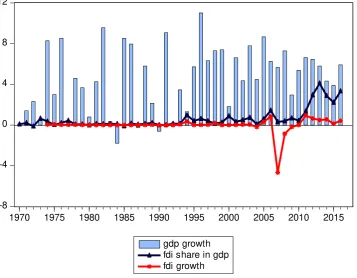
Table 1 provides some basic statistics for GDP growth, FDI share in GDP and FDI

growth for 5 sub-periods between 1970 and 2016 whereas Figure 1 presents the time series

plots of the variables over the entire sample period of 1970-2016. As can be observed the lowest

economic growth rates and the FDI growth figures occurred between the first two sub-periods

dating over 1970-1990, with minimum GDP growth values 1.78%) and FDI share in GDP

(-0.092) occurring in 1984-1985. Following democratic transitions experienced in the early

1990’s resulted in significantly improved economic growth performance with GDP growth

rates experiencing an all-time high of over 11 percent in 1996 with FDI’s growing significantly

yet remaining relatively low in terms of wold standard/averages. Notably, FDI growth

plummeted during the more recent global financial crisis of 2007-2008, reaching an extreme

low of -4.66% in 2007, and yet following the Gold sector boom of 2010, FDI have experienced

since gaining independence in the 1960’s reaching growth levels of 0.95% in 2011 and over a

4% share in GDP in 2013.

Table 1: Basic GDP growth and FDI statistics

Time series variables

GDP FDI FDI_GDP

Panel A: Mean values

1970-2016 4.588 -0.008 0.324

1970-1979 3.050 0.037 0.184

1980-1989 3.600 0.004 0.098

1990-1999 5.759 0.071 0.401

2000-2009 5.945 -0.457 0.548

2010-2016 5.502 0.537 2.806

Panel B: Maximum and minimum values

Minimum -1.779 [1984] -4.656 [2007] -0.092 [1985]

Note: Year associated with maximum and minimum values reported in brackets [].

Figure 1: GDP growth, FDI share in GDP and FDI growth in Burkina Faso

-8 -4 0 4 8 12

1970 1975 1980 1985 1990 1995 2000 2005 2010 2015

gdp growth fdi share in gdp fdi growth

3. Literature Review

Empirical work on dynamic models of economic growth can be traced to seminal papers

of Harrod (1939) and Domar (1946) which became more prominently branded as the

neo-classical synthesis following later contributions of Nobel laurate Solow (1965).Whilst capital accumulation is defined as the engine of growth within such dynamic models, initially there

was very little role for foreign capital flows in influencing long-term dynamic growth. This is

because conventional neoclassical models are built on the foundation of constant returns to

scale in the production function which results in increased capital accumulation producing

diminishing returns to capital. Under the assumption of diminishing returns to capital, FDI is

merely an injection of capital stock which can only affect the level of income, leaving the

Eventually, endogenous growth model, as attributed to seminal contributions of Lucas

(1988) and Romer (1986, 1987, 1990), took centre stage within the dynamic growth paradigm

in which the key determinants of growth are endogenous to the model. These ‘endogenous

growth models’ generally assume constant returns to scale for input factors with the level of

technological progress being a form of investment spillover dependent upon a set of factors,

such as tangible capital, human capital and research and development (Belloumi, 2014).

Henceforth within endogenous growth models, long-run steady-state growth can be achieved if

the marginal product of capital can be bounded away from the rate of time preference as the

stock of foreign capital flows increases, such that the long-run growth rate positively depends

on foreign capital (de Mello, 1999). Theoretically, some identified channels through which FDI can improve steady-state growth within endogenous models include increased capital

accumulation in the recipient economy, include improved efficiency of locally owned host

country firms via contract and demonstration effects, and their exposure to fierce competition,

technological change, human capital augmentation and increased exports (Akinlo, 2005).

On the other hand, potential drawbacks of FDI on any economy’s growth have also

being identified in the literature. For instance, Hansen and Rand (2006) earlier highlighted the

possibility of FDI Deteriorating of the Balance of Payments as profits are repatriated thus

exerting adverse effects on competitiveness in domestic markets. Adams (2009) further

concludes that for the case of developing and especially African countries, FDI can spur economic development only after some basic conditions are meet since the impact of FDI is

constrained by an absorptive capacity in terms of availability of trained workers, basic

infrastructure network and institutions as well as macroeconomic performance. Therefore,

while FDI can potentially stimulate economic growth, these growth effects are only sustainable

if FDI stimulates the utilization of domestic factors of production, especially by increasing

employment and stimulating domestic public as well as private investment (Baharumshah and

Almasaied, 2009).

different methodologies used as well as the empirical findings of the different studies. In

quickly screening through these studies, we can conveniently segregate these studies into three

classifications. The first group consists of a majority of studies which find a positive

relationship between FDI and economic growth (i.e. Seetanah and Khadaroo (2007), Sharma

and Abekah (2008), Ndikumana and Verick (2009), Brambila-Macias and Massa (2010), Loots

and Kabundi (2012) and Adams and Klobodu (2012)). The second group of studies are those

which found an insignificant FDI-growth relationship for the data (i.e. Ndambendia and

Njoupouognigni (2010), Seyoum et al. (2014), Tomi (2015)). There is the third cluster of studies

which find a significant and inverse relationship between the two time series (i.e. Adams (2009)

and Ndiaye and Xu (2016)). The general inconclusiveness of the aforementioned studies leaves the subject matter open to further deliberations. A natural development to the above literature

would be to provide country-specific evidence for Burkina Faso.

Table 2: Summary of reviewed literature

Author Period Country Method Results Lumbila (2005)

1980-2000

47 African countries

SUR-WLS FDI positively and significantly affects economic growth except for panels with

high inflation rates and high corruption levels.

Sharma and Abekah (2008)

1990-2003

47 African countries

POLS FDI has a positive and significant effect on economic growth for the entire panel. Ndikumana and Verick (2009) 1970-2004 38 SSA countries

Pesaran coefficient, POLS, FE. FDI inflows are significantly and positively correlated with a range of determinants

including GDP growth Adams (2009)

1990-2003

42 African countries

POLS and FE Significant and positive relationship between FDI and growth using OLS and

insignificant using FE. Brambila-Macias and Massa (2010) 1980-2008 45 African countries

DOLS FDI has a positive and significant effect on economic growth for the entire panel. Ndambendia and Njoupouognigni (2010) 1980-2007 36 SSA countries

PMG and FE FDI has an insignificant effect on economic growth for all estimators. Brambila-Macias and Massa (2010) 1980-2007 45 SSA countries

DOLS FDI positively affects GDP for entire sample.

Loots and Kabundi (2012)

2000-2007

46 African countries

POLS and FE Positive relationship between FDI and economic growth Tekin (2012)

1970-2009

18 least developed

countries

Panel bootstrap granger causality tests

Causality from economic growth for FDI in Burkina Faso but not vice versa. Gui-Diby (2014)

1980-2009

50African countries

GMM Significant negative relationship between FDI and economic between 1980-1999 and

significant positive relationship between FDI and economic between 1995-2009. Seyoum et al. (2015)

1970-2011

23 African countries

LA-VAR model No causality between FDI and economic growth for Burkina Faso Tomi (2015)

1970-2012

7 WAEMU countries

Ndiaye and Xu (2016) 1990-2012

7 WAEMU countries

POLS and FE Regression results report a negative and significant relationship between FDI and

GDP Adams and Klobodu

(2017)

1970-2014

5 SSA countries

ARDL There is a positive and significant relationship between FDI and economic

growth Burkina Faso

Notes: POLS – Panel ordinary least squares; LA-VAR – Lag augmented vector autoregressive model; ADRL – Autoregressive distributive lag model; PMG – Pooled Mean group; FE – Fixed effects, SUR-WLS – Seemingly Unrelated Regression weighted least squares; GMM – Generalized Method of Moments.

4. Empirical framework

The theoretical model used in this study draws heavily from the growth model specified in De Mello (1997), Bosworth and Collins (1999), Ramirez (2000) and Akinlo (2004). In the

model FDI is incorporated as externality within the following production function:

Yt = Af {(L), Kp, } = Af (Hz) = At (L)α𝐾_𝑝 

, 1-α-, α +  < 1 (1)

Where Yt is real output, A is the efficiency of production, Kp is domestic capital stock,

L is labour input,  is level of human capital, α is the private capital share,  is labour share and

 is the externality generated by increased FDI. Denoting Kf as the foreign capital flows as well

as  and  as the marginal and intertemporal elasticities of substitution between private

domestic and foreign capital, respectively,  can be expressed as by the following

Cobb-Douglas function:

 = {(L)Kp, 𝐾_𝑓 }  > 0,  > 0 (2)

And substituting equation (2) into (1) produces:

Yt = At (L)α𝐾_𝑝 

[{(L)Kp, 𝐾_𝑓 }}]1- α -  (3)

Yt = Af {(HzL)α + (1- α - )Kp + (1- α - ) Kf(1- α - ) (4)

And in defining  = Hz, with H denoting a measure of educational level and z is the returns to education relative to labour input, L, the general growth accounting equation which

can be derived from equation (4) is given as:

Gy = gA+ z(α + –α - )gH+ (α + –α - )gL + ( + –α - )gkp + (–α - )gkp

(5)

And in further log-linearizing equation (5), we obtain the following empirical

regression:

y = 0 + 1kp + 2kf + 3h + et (6)

Where 0 is a regression intercept, the lowercase letters represent the natural logarithmic

transformations of the variables and et is a well-behaved disturbance term. De Mello (1997),

Bosworth and Collins (1999), Ramirez (2000) and Akinlo (2004) have all argued for the

baseline empirical regressions can be augmented with a vector X, which denotes a vector of

control variables i.e.

y = 0 + 1kp + 2kf + 3h + 4X + et (7)

In alignment with Barro (1991), De Long and Summers (1991), Levine and Renelt

(1992), Barro and Sala-i-Martin (1995) and Sala-i-Martin (1997) popular choices for the growth

control variables as found in the literature include government size (Iamsiraroj and Ulubasoglu,

2015), inflation (Lumbila, 2005), financial deepening (Akinlo, 2004), urbanization (Alguacil et

al., 2011), exports (Adams, 2009) and exchange rates (Li and Lui, 2004). Equation (7) can be

estimated in a straightforward manner using OLS estimates (see Sharma and Abekah (2008),

model (VECM) (see de Mello (1997, 1999), Akinlo (2005)). As mentioned before, our study

relies on the ARDL model of Peseran et al. (2001) which has gained popularity over other

contending cointegration models on the premise of i) allowing for modelling of time series

variables whose integration properties are either I(0) or I(1) ii) the models suitability with small

sample sizes and iii) the model providing unbiased estimates of the long-run model even when

some of the estimated regressors are endogenous. The ARDL representation of the equation (7)

can be reformulated as:

_{𝑦𝑡 =}_{0 + ෍}𝑝 _1𝑖

𝑖=1 𝑘𝑝𝑡−𝑖+ ෍ 2𝑖

𝑝

𝑖=1 𝑘𝑓𝑡−𝑖+ ෍ 3𝑖

𝑝

𝑖=1 ℎ𝑡−𝑖+ ෍ 4𝑖

𝑝

𝑖=1 𝑋𝑡−𝑖+

_{1𝑖𝑘𝑝𝑡−𝑖+}_{2𝑖𝑘𝑓𝑡−𝑖+}_{3𝑖ℎ𝑡−𝑖+}_{4𝑖𝑋𝑡−𝑖+ +}_𝑡 (8)

Where  is a first difference operator, 0 is the intercept term, the parameters 1, …, 4

and 1, …, 4 are the short-run and long-run elasticities, respectively, and t is a well-behaved

error term. From equation (8), the bounds test for cointegration can be implemented

straightforward by testing the null hypothesis of no cointegration (i.e. 1 = 2 = 3 = 4 = 5 = 6

= 0), which is tested against the alternative hypothesis of ARDL cointegration effects (i.e. 1≠

2 ≠ 3 ≠ 4 ≠ 5 ≠ 6 ≠ 0). There cointegration test is evaluated via a F-statistic, of which the

null hypothesis of ARDL cointegration effects are rejected if the computed F-statistic exceeds

the upper critical bound and cannot be rejected if the F-statistics is less than the lower critical

bound level. However, if the F-statistic falls between the upper and lower critical bound, then

the cointegration tests are deemed as inconclusive. Once cointegration effects are validated, then the following unrestricted error correction model (UECM) representation of the ARDL

regression (8) can be modelled as follows:

_{𝑦𝑡 =}_{0 + ෍}𝑝 _1𝑖

𝑖=1 𝑘𝑝𝑡−𝑖+ ෍ 2𝑖

𝑝

𝑖=1 𝑘𝑓𝑡−𝑖+ ෍ 3𝑖

𝑝

𝑖=1 ℎ𝑡−𝑖+ ෍ 4𝑖

𝑝

𝑖=1 𝑋𝑡−𝑖+

+ _{𝑒𝑐𝑡𝑡−𝑖+}

Where ectt-1 is the error correction term which measures the speed of adjustment of the

series towards steady-state equilibrium in the face of disequilibrium. Pragmatically, the error

correction term should be negative and statistically significant in order for the short-run

dynamic effects to translate into meaningful long-run effects.

5. Data and empirical results

5.1Empirical data

Deriving directly from theoretical model and its augmentation of control variables, our

study makes use of 8 time series variables (i.e. GDP growth, FDI, domestic investment,

secondary schooling, inflation, urbanization and exports). Table 3 provides details of the time

series variables used in our empirical study and particularly shows their description, their

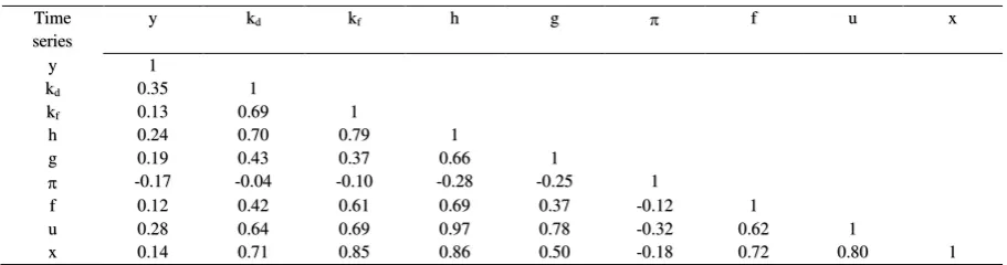
coverage period as well as their source. Table 4 presents the correlation matrix of the time series

and can be easily observed all variables are positively correlated with economic growth with

the sole exception of inflation. We note that these preliminaries reported in Table 4 confine to

standard growth theory.

Table 3: Description of time series variables

Symbol Time series Coverage Period Source y Annual % growth rate of GDP at

market prices

1970-2016 World Bank

kp Gross fixed capital formation as %

of GDP

1970-2016 World Bank

kf Foreign direct investment, net

inflows as % of GDP

1970-2016 World Bank

h Secondary school enrolment (gross %)

1970-2016 World Bank

g General government final consumption expenditure as % of

GDP

1970-2016 World Bank

 Inflation in consumer prices (annual %)

1970-2016 World Bank

u Urban population as % of total population

x Exports of goods and services as % of GDP

1970-2016 World Bank

Note: All employed time series have been transformed into their natural logarithms for

empirical purposes.

Table 4: correlation matrix

Time series

y kd kf h g  f u x

y 1

kd 0.35 1

kf 0.13 0.69 1

h 0.24 0.70 0.79 1

g 0.19 0.43 0.37 0.66 1

 -0.17 -0.04 -0.10 -0.28 -0.25 1

f 0.12 0.42 0.61 0.69 0.37 -0.12 1

u 0.28 0.64 0.69 0.97 0.78 -0.32 0.62 1

x 0.14 0.71 0.85 0.86 0.50 -0.18 0.72 0.80 1

5.2Unit root tests

Even though unit root testing is not a pre-condition for the implementation of the ARDL model, we take caution in ensuring that none of the time series is integrated of order higher than

I(1). Table 4 presents the empirical results of the DF-GLS (Elliot et al. 1996) and the Ng-Perron

(Ng and Perron, 1996, 2001) unit root tests performed on the first differences of the time series.

We avoid the use of popular, conventional unit root testing procedures such as the ADF (i.e.

Dickey and Fuller, 1979), PP (i.e. Philips and Perron, 1988) and KPSS (i.e. Kwiatkowski et al.,

1992) since it is well acknowledged that these traditional testing procedures exhibit lower

power in distinguishing between unit root processes and close-to-unit root behaviour and

further suffer from unfavourable small sample size properties. The tests presented by Elliot et

al. (1996) and Ng and Perron (1996, 2001) circumvent these criticisms and are based on local

de-trending techniques which display good power properties in small samples. This latter point is relevant for each of our series which only consists of 37 observations.

To implement the aforementioned tests it is imperative to select an appropriate lag

length for the ‘autoregressive trunculation’ which are included to soak up possible serial

correlation in the errors of the testing regressions. Ng and Perron (1995, 2001) suggest the use

we apply this principle by setting a maximum of 9 lags on the test regression and trim down

until lag 0. Our optimal lag is selected as that which minimizes the MAIC values. Panel A of

Table 5 reports the findings from these ‘modified’ tests performed with only a drift on our series

whereas Panel B does so for the tests performed with both a drift and intercept. As can be

observed from Table 5, there is overwhelming evidence rejecting the unit root hypothesis for

the employed time series in their first differences which the exception of the results obtained

from the DF-GLS test performed with a drift on GDP, urbanization and exports as well as the

DF-GLS test performed with both a drift and trend on domestic investment and urbanization.

Against this evidence, we proceed to model and estimate our empirical ARDL regressions.

Table 5: Unit root tests on the first differences of the time series

DF-GLS MZa MZt MSB MPT Panel A: drift

y 0.91

[6] -38.49*** [1] -4.38*** [1] 0.11*** [1] -38.49*** [1] kd -0.59***

[8] -21.58*** [0] -3.25*** [0] 0.15*** [0] 1.25*** [0] kf -10.26***

[0] -34.48*** [1] -4.15*** [1] 0.12*** [1] 0.72*** [1]

h -3.45

[0] -14.16*** [0] -2.66*** [0] 0.18** [0] 1.73*** [0] g -7.66***

[0] -45.13*** [1] -4.75*** [1] 0.11*** [1] 0.54*** [1]  -14.39***

[0] -26.40*** [1] -3.63*** [1] 0.14*** [1] 0.93*** [1] f -3.06***

[2] -19.97*** [0] -3.16*** [0] 0.16*** [0] 1.24*** [0]

u -0.88

[2] -33.09*** [1] -4.07*** [1] 0.12*** [1] 0.74*** [1]

x -1.18

[6] -21.74*** [0] -3.29*** [0] 0.15*** [0] 1.13*** [0] Panel B: drift

and trend

y -12.13*** [0] -44.85*** [1] -4.73*** [1] 0.11*** [1] 2.05*** [1] kd -1.51

[8] -21.70*** [0] -3.29*** [0] 0.15** [0] 4.20** [0] kf -10.27***

[0] -34.62*** [1] -4.16*** [1] 0.12*** [1] 2.64*** [1] h -4.34***

[0] -16.28*** [0] -2.85* [0] 0.17* [0] 5.63** [0] g -7.72***

[0] -46.62*** [1] -4.82*** [1] 0.10*** [1] 1.96*** [1]  -14.42***

[0] -26.64*** [1] -3.65*** [1] 0.14*** [1] 3.42*** [1] f -4.75***

[0] -20.19*** [0] -3.17*** [0] 0.16*** [0] 4.56*** [0]

u -3.86

[0] -33.52*** [1] -4.09*** [1] 0.12*** [1] 2.72*** [1] x -6.08***

Notes: “***’, ‘**’, ‘*’ denote the 1%, 5% and 10% critical levels, respectively. Optimal lag length as

determined by the modified AIC reported in [].

5.3Cointegration tests

We begin our modelling process of the ARDL models by choosing the appropriate lag

length for each estimated regressions. This is achieved by finding the ARDL regression which

minimizes the Schwarz’s criterion (SC). Note that we have a total of 7 estimated regressions,

the first being the log-linear baseline growth model as represented in equation (6), the second

to the sixth equations being the baseline model inclusive of one control variable and the last

equation being the baseline model inclusive of all control variables. The optimal lag lengths for

each obtained for each of our regressions is reported in second column of Table 5 and all

regressions indicate an optimal lag length of 1 on the dependent variable and 0 lags being

optimal for all intendent variables. This finding is plausible considering the short-sample of

time series. The corresponding bounds test for cointegration for the ARDL regressions are

reported in the third column of Table 6. As can be observed, all produced F-statistics exceed

their respective 1 percent upper bound critical levels hence strongly rejecting the null

hypothesis of no ARDL cointegration effects.

Table 6: Bounds test for cointegration tests

function Equation No. Lag selection Test statistics

Critical values

10% 5% 1% I(0) I(1) I(0) I(1) I(0) I(1) f(y~kf, kd, h) 1 (1,0,0,0) 17.17*** 2.72 3.77 3.23 4.35 4.29 5.61

f(y~kf, kd, h,

g)

2 (1,0,0,0,0) 13.96*** 2.45 3.52 2.86 4.01 3.74 5.06 f(y~kf, kd, h,

)

3 (1,0,0,0,0) 13.43*** 2.45 3.52 2.86 4.01 3.74 5.06 f(y~kf, kd, h,

f)

4 (1,0,0,0,0) 13.37*** 2.45 3.52 2.86 4.01 3.74 5.06 f(y~kf, kd, h,

u)

5 (1,0,0,0,0) 14.71*** 2.45 3.52 2.86 4.01 3.74 5.06 f(y~kf, kd, h,

x)

6 (1,0,0,0,0) 13.49*** 2.45 3.52 2.86 4.01 3.74 5.06 f(y~kf, kd, h,

g, , f, u, x)

7 (1,0,0,0,0,0,0,0,0) 7.33*** 1.95 3.06 2.22 3.39 2.79 4.10

5.4Regression results

Having confirmed bounds cointegration effects for our regressions, we now present the empirical estimates of our six empirical regressions in Table 7 whereas the associated

diagnostic tests are found in Table 8. In referring to the long-run estimates reported in Panel A

of Table 7, we find statistically significant coefficients on the investment variable across the

six estimated regressions. This finding is evidently consistent with traditional growth theory

which views capital accumulation as the engine of dynamic economic growth. However, in

turning to our main growth determinant, the FDI variable, we observe negative and statistically

significant coefficient estimates in equation (1), equation (2) and equation (5) whereas in the

remaining regressions the FDI coefficient either produces a negative and insignificant estimates

(i.e. equations (3), (4) and (7)) or a negative and insignificant estimates (i.e. equation (6)).

Clearly, these latter results oppose those of conventional thinking and yet are in line with those

previously presented by Ndambendia and Njoupouognigni (2010), Seyoum et al. (2014) and Tomi (2015), for similar West African data.

Other findings which are at odds with conventional growth theory include the

insignificant coefficient estimates on the government expenditure variable (i.e. equation (2)),

the inflation variable (i.e. equation (3)), the financial deepening variable (i.e. equation (4) as

well as the urbanization variable (i.e. equation 5). We also observe insignificant coefficient

estimates on the schooling time series in most regressions (i.e. equations (1), (2), (3), (4), (5),

and (7)) except for equation 6, where the schooling variable produces the theoretically correct

positive and statistically significant estimate. Note, that these findings are in line with those

found in previous literature of Adams (2009) as well as Gui-Diby (2014). Encouragingly enough, we able to establish a positive and statistically significant coefficient estimate on the

exports variable (i.e. equation (6) and (7)), which we note is in accordance with traditional

growth theory as well as previous empirical evidence presented by Adams (2009), Seyoum et

al. (2015) and Ndiaye and Xu (2016). We finally note that the short-run estimates reported in

panel B of Table 6 seemingly mirror those of the long-run in Panel A in terms of the sign and

to (7) produce a correct negative and statistically significant value implying equilibrium

correction behaviour in the face of an exogenous shock to the series.

Table 7: Empirical regression estimates (dependent variable: y)

1 2 3 4 5 6 7

Panel A: Long-run

kd 0.24*

(0.06) 0.24* (0.09) 0.26* (0.05) 0.25* (0.07) 0.24* (0.08) 0.27** (0.02) 0.31** (0.03) kf -0.72*

(0.09) -0.91* (0.09) -0.72 (0.11) -0.76 (0.18) -0.97* (0.07) 0.11 (0.82) -0.09 (0.87) h 0.61

(0.16) 1.26 (0.26) 0.47 (0.38) 0.58 (0.26) -1.02 (0.66) 1.03** (0.01) -0.87 (0.78)

g -0.11

(0.52)

-0.03 (0.86)

 -0.04

(0.50)

-0.03 (0.48)

f 0.02

(0.88)

0.11 (0.41)

u 0.25

(0.48)

0.29 (0.45)

x 0.22*

(0.03)

0.32** (0.03) Panel B:

Short-run

kd 0.31*

(0.05) 0.31* (0.08) 0.33* (0.04) 0.31* (0.07) 0.30* (0.08) 0.36** (0.01) 0.42** (0.03) kf -0.91*

(0.08) -1.15* (0.08) -0.89* (0.09) -0.97 (0.17) -1.22* (0.07) 0.15 (0.82) -0.12 (0.87) h 0.77

(0.15) 1.58 (0.26) 0.59 (0.38) 0.73 (0.25) -1.29 (0.67) 1.37** (0.01) -1.18 (0.79)

g -0.14

(0.52)

-0.04 (0.86)

 -0.05

(0.49)

-0.05 (0.47)

f 0.02

(0.88)

0.15 (0.40)

u 0.31

(0.49)

0.40 (0.46)

x 0.29**

(0.03)

0.44* (0.03) Ect(-1) -1.26***

(0.00) -1.25*** (0.00) -1.25*** (0.00) -1.26*** (0.00) -1.26*** (0.00) -1.33*** (0.00) -1.36 (0.00)*** R2 _{0.23 0.24 0.24 0.23 0.24 0.28 0.34}

Notes: “***’, ‘**’, ‘*’ denote the 1%, 5% and 10% critical levels, respectively.

5.5Sensitivity analysis

In this subsection of the paper, we present a sensitivity analysis with the following modifications being made to our original estimated regressions. Firstly, we employ a different

measure of FDI, with the growth in FDI being used in place of FDI as a share in GDP. Secondly,

2009, a period in which FDI growth was in negative figures for these three consecutive years.

Thirdly, we add, a number of interactive terms within the estimated regression and these are

intended to capture the interaction effects between i) fdi and domestic investment (equation (1))

ii) fdi and human capital (equation (2)) iii) fdi and government size (equation (3)) iv) fdi and

financial deepening (equation (4)) v) fdi and urbanization (equation (5)) ii) fdi and exports

(equation (6)). Lastly, we remove the inflation variable from all regressions as the inclusion of

the time series in all regression fails to secure any significant ARDL cointegration effects.

The results of the sensitivity analysis presented in Table 8, indicate that all seven

estimated regressions display significant cointegration effects between the time series as evidence from the F-statistics of the bounds tests reported in Panel A points to the null

hypothesis of no cointegration null hypothesis being rejected at significance levels of at least 5

percent for equations (1) through (7). The long-run estimates reported in Panel B produce

familiar positive and significant estimates on the investment variable (equations (1) – (7)) and

export variables (equations (6) – (7)). We also establish two statistically significant estimates

for the schooling variable, one positive (equation (6)) and the other negative (equation (7)),

hence rendering the evidence as inconclusive. Moreover, the dummy variable only produces

the expected negative and statistically significant estimate in regression (7), thus providing

evidence on the adverse effects of the 2009 global financial collapse on the Burkina Faso

economy. The remainder of the long-run coefficients (i.e. interactive terms, government size, financial deepening) are all statistically insignificant across all estimated regressions.

Concerning the short-run estimates reported in Panel C, the only exceptional finding from our

previous estimates is the positive and statically significant estimate on the on the interactive

term between fdi and exports (i.e. equation (7)), a finding which is more in lieu with

Table 8: Sensitivity estimates (dependent variable: y)

1 2 3 4 5 6 7

Panel A: Bounds test

ARDL specification

(1,0,0,0,0,0) (1,0,0,0,0,0) (1,0,0,0,0,0) (1,0,0,0,0,0) (1,0,0,0,0,0) (1,0,0,0,0,0) (1,0,0,0,0,0) F-statistic 9.49*** 9.92*** 8.40*** 8.66*** 8.57*** 8.97*** 4.34**

Panel B: Long-run

kd 0.28*

(0.06) 0.25* (0.06) 0.24* (0.08) 0.25* (0.07) 0.29** (0.01) 0.34*** (0.00) 0.53*** (0.00) kf -0.16

(0.95 -0.52 (0.80) 1.34 (0.77) -0.42 (0.79) -2.96 (0.20) -2.04 (0.32) 0.01 (0.98) h 0.06

(0.40) 0.08 (0.29) 0.07 (0.46) 0.07 (0.39) -0.35*** (0.00) 0.29*** (0.00) -0.34 (0.28)

g 0.04

(0.68)

-0.16 (0.19)

f 0.04

(0.74)

0.13 (0.25)

u 0.42***

(0.00)

0.70* (0.04)

x 0.49***

(0.00)

0.72** (0.01) Dum -0.38

(0.63) -0.48 (0.56) -0.43 (0.66) -0.41 (0.61) -0.35 (0.58) -2.56*** (0.00) -1.82 (0.10) fdi  kd -0.03

(0.76)

-0.40** (0.01) fdi  h -0.02

(0.81)

-0.37 (0.32)

fdi  g -0.11

(0.62)

-0.05 (0.65)

fdi  f -0.03

(0.72)

-0.09 (0.43)

fdi  u 0.10

(0.21)

0.40 (0.15)

fdi  x 0.07

(0.35)

0.61 (0.10) Panel C:

Short-run

kd 0.31*

(0.08) 0.30* (0.07) 0.27 (0.12) 0.35* (0.04) 0.36** (0.03) 0.40** (0.01) 0.59*** (0.00) kf -0.49

(0.87) -2.09 (0.31) 0.07 (0.98) -3.17 (0.19) -5.07* (0.09) -4.12* (0.05) -11.06 (0.16) h 0.03

(0.94) -0.06 (0.89) -0.01 (0.97) -0.15 (0.75) -0.62 (0.40) 0.46 (0.28) 0.96 (0.34)

g 0.19

(0.49)

0.19 (0.53)

f 0.03

(0.92)

-0.02 (0.96)

u 0.84

(0.54)

-0.37 (0.81)

x 0.97***

(0.00)

1.38*** (0.00) fdi  kd -0.02

(0.88)

0.41* (0.05) fdi  h 0.06

(0.54)

-1.75** (0.02)

fdi  g -0.05

(0.83)

-0.20 (0.58)

fdi  f 0.12

(0.34)

0.32 (0.27)

fdi  u 0.18

(0.15)

1.35* (0.06)

fdi  x 0.19*

(0.06)

Dum 1.49 (0.51) 1.18 (0.59) 1.22 (0.58) 1.28 (0.56) 0.61 (0.77) -2.65 (0.23) -2.76 (0.23) Ect(-1) -1.34***

(0.00) -1.32*** (0.00) -1.35*** (0.00) -1.32*** (0.00) -1.32*** (0.00) -1.39*** (0.00) -1.62*** (0.00) R2 _{0.21 0.21 0.22 0.22 0.29 0.32 0.51}

Notes: “***’, ‘**’, ‘*’ denote the 1%, 5% and 10% critical levels, respectively.

5.6Diagnostic tests and stability analysis

In order to validate the estimates presented in the previous sub-section, we apply a

battery of diagnostic tests to ensure that the residuals conform to the classical regression

assumptions. These diagnostics include tests for normality in regression residuals, tests for

serial correlation in regression errors, tests for heteroscedasticity between the errors and the

regressand variables, tests for correct functional form as well as CUSUM and CUSUM of squares plots for stability of estimated regressions. The results of these test performed on our

original regressions are reported in Panel A of Table 9 and indicate that all regressions conform

to the classical regressions assumptions. The same can be concluded for the sensitivity analysis

estimates as presented in Panel B of Table 9 with the sole exception of regression (3), in which

both CUSUM and CUSUM of squares plots indicate instability of the regression at a 5 percent

critical level.

Table 9: Residual diagnostics and stability analysis

Panel A: Original regressions

Equation 1 2 3 4 5 6 7

Norm 0.53 (0.77) 0.32 (0.85) 0.40 (0.82) 0.15 (0.93) 0.23 (0.89) 0.29 (0.87) 0.49 (0.78)

SC 0.14

(0.87) 1.16 (0.35) 1.71 (0.16) 1.65 (0.17) 1.39 (0.26) 1.84 (0.18) 2.18 (0.13) Het. 0.86

(0.47) 0.70 (0.41) 0.75 (0.39) 0.28 (0.60) 1.22 (0.32) 1.58 (0.18) 1.48 (0.21)

FF 0.95

(0.35) 0.02 (0.98) 0.25 (0.80) 0.42 (0.68) 0.15 (0.898) 0.70 (0.49) 0.52 (0.61)

CUSUM S S S S S S S

CUSUMSQ S S S S S S S

Panel B: Sensitivity regressions

Equation 1 2 3 4 5 6 7

Norm 0.88 (0.64) 0.76 (0.68) 0.68 (0.71) 0.04 (0.98) 1.39 (0.50) 0.76 (0.68) 2.13 (0.35)

SC 0.53

(0.78) 0.77 (0.60) 1.09 (0.39) 0.79 (0.60) 0.02 (0.96) 0.60 (0.75) 1.14 (0.34) Het. 0.81

FF 0.54 (0.60)

0.71 (0.49)

0.36 (0.72)

0.42 (0.68)

0.11 (0.91)

0.57 (0.58)

1.59 (0.12)

CUSUM S S U S S S S

CUSUMSQ S S U S S S S

Notes: S – stable and U – unstable

6. Discussion of results

Our empirical results obtained in the previous section presents a number of interesting

phenomenon concerning the Burkina Faso. Starting with the findings from the control variables

used the multivariate regressions, the common finding of a a positive investment-growth, a

positive urbanization-growth as well as a positive trade-growth relationship are consistent with

traditional economic theory which view domestic investment as the engine of growth (Solow;

1965; Swan 1965; Rommer 1988), urbanization as an indicator of infrastructure in

communication and transportation (Barro and Salai-i-Martin, 1995; Salai-i-Martin, 1997) and

trade as the ‘newer’ engine of growth which must exploited by developing and emerging

economies to induce catch-up effects (Riedel, 1988). However, given the current global

environment of falling and unstable world prices, futures income expected from exports may be undermined which may further worsen the current economic woes faced by Burkina Faso

economy.

Empirical findings which are at odds with conventional economic theory include that of

an insignificant government size-economic growth relationship which is contradictory to

Wagner’s hypothesis of a positive relationship between the variables. However, Adam and

Klobodu (2017) have established similar negative government size-growth relationships for

previous FDI-growth studies for West African countries. Notably the nonlinear dynamics of the

government size-growth relationship, as advocated by Barro (1990), Armey (1995), Rahn and

Fox (1996) and Scully (1995) may explain this phenomenon as the economy may have crossed

the threshold at which government spending is useful to economic prosperity. Other aspects such as corruption and inefficient use of government funds may contribute to this finding of

The insignificant relationship found between inflation and economic growth is

reminiscent of the ‘superneutrality hypothesis of money’ in which monetary policy action can

only affect nominal variables such as inflation and money supply without influencing real

variable such as capital accumulation and economic growth (Sidrauski, 1967). Henceforth, the

country’s affiliation with the West African, Economic and Monetary Union (WAEMU) which

ensure a financial stable environment, cannot solely guarantee an environment conducive for

economic growth. Other unconventional findings include insignificant effects of school

attainment and financial deepening towards the growth of the economy and these are opposing

to existing theoretical and empirical propositions (Schumpter 1912; Barro (1991); De Long and

Summers (1991); Levine and Renelt (1992)). We attribute this irregularities to deeper socio-structural imbalances existing within the Burkina Faso economy.

In the same vein, the insignificant relationship found between our primary growth

explanatory variable, FDI, and economic growth, is contrary to the traditional economy belief

and its low impact may be attributed to its historic low share in GDP. In turn, low FDI levels

may be attributed to low investor confidence in Burkina Faso amidst her legacy of severe

political instability which is easily observable from the number of coups experienced by the

country over the last couple of decades. The positive and significant interaction between FDI

and exports in promoting short-run economic growth, reflects the importance in which the

available external financial inflows contribute towards enhancing export-oriented growth for products such as cotton and cereals. Nevertheless, the spillover effects of FDI towards

technological infrastructure, as it’s interaction with urbanization, as well as enhanced human

development, as reflected with FDI’s interaction with schooling attainment, are virtually non

-existent over both the short and long-run. Moreover, that lack of interaction between FDI and

government size may also indicate the inefficiency of fiscal structure and expenditure towards

infrastructure projects conducive for attracting FDI. Altogether, we believe that our results

resonate from the country’s legacy of political instability and resulting low investor’s

confidence and willingness to invest in the economy.

The main objective of the study was to examine the short-run and long-run cointegration

relationship between FDI and Economic growth in Burkina Faso using time series spanning

between 1970 and 2016 applied to the ARDL model of Peseran et al. (2001). Our estimate

empirical model is directly derived from endogenous growth setting in which FDI may exert

direct as well as indirect, spillover effects on steady-state growth via human capital

development, enhanced domestic investment, increased government spending mainly in

infrastructure as well as through technology advancements reflected in higher urbanization and

export production. Whilst we are unable to find any significant effects of FDI on growth over

the long-run, we are, however, able to establish positive interactive effects of FDI on export size towards economic growth over the short-run.

The general lack of a finding of significant effects of FDI on long-run economic growth

in Burkina Faso reflects the historically low share of FDI in economic growth caused by

previous policies of nonalignment with western countries. Another contributing factor to these

findings is the lack of investor confidence due to decades of political instability reflecting in

the numerous coups in Burkina Faso. And in considering the advent of the most recent coup

attempts and terrorist bombings in 2015, the confidence of potential foreign investors is most

likely to be further dampened. Domestic authorities should thus be primarily concerned with

implementing policies and socio-economic strategies aimed at enhancing a politically stable environment as a means of securing international confidence in the country.

References

Adams S. (2009), “Foreign direct investment, domestic investment, and economic growth in

Sub-Saharan Africa”, Journal of Policy Modeling, 31, 939-949.

Adams S. and Klobodu E. (2017), “Capital flows and economic growth revisited: Evidence

Akinlo A. (2004), “Foreign direct investment and growth in Nigeria An empirical investigation”, Journal of Policy Modeling, 26, 627-639.

Alguacil M., Cuadros A. and Orts V. (2011), “Inward FDI and growth: the role of

macroeconomic and institutional environment”, Journal of Policy Modeling, 33(3), 481-496.

Armantier O. and Boly A. (2013), “Comparing corruption in the laboratory and in the field in

Burkina Faso and in Canada”, The Economic Journal, 132(573), 1168-1187.

Armey D. (1995), “The freedom revolution: Why big government failed, why freedom works,

and how we will rebuild America”, Washington, DC: Regnery Publishing.

Balasubramanyam V., Salisu M. and Sapsford D. (1999), “Foreign direct investment as an engine of growth”, Journal of International Trade and Economic Development, 8(1), 27-40

Baharumshah A. and Almasaied S. (2009), “Foreign direct investment and economic growth in

Malaysia: Interactions with human capital and financial deepening”, Emerging Markets

Finance and Trade, 45(1), 90-102.

Barro R. (1990), “Government spending in a simple model of endogenous growth”, Journal

of Political Economy, 98, 103-126.

Barro R. (1991), “Economic growth in a cross section of countries”, Quarterly Journal of

Economics, 106(425), 407-443.

Barro R. and Sala-i-Martin X. (1995), “Economic growth”, New York: McGRaw-Hill.

Bosworth B. and Collins S. (1999), “Capital flows to developing economies: Implications for

saving and investment”, Brookings Papers on Economic Activity, 1, 143-180.

De Long and Summers (1991), “Equipment Investment and economic growth”, The Quarterly

Journal of Economics, 106(2), 445-502.

de Mello L. (1997), “Foreign direct investment in developing countries and growth: A

selective survey”, Journal of Development Studies, 34, 1–34.

de Mello L. (1999), “Foreign direct investment-led growth: Evidence from time series and panel

data”, Oxford Economic Papers, 51, 133–151.

Dickey D. and Fuller W. (1979), “Distribution of the estimators for autoregressive time series with a unit root”, Journal of the American Statistical Association, 74(366), 427-431.

Domar D.E. (1946), “Capital expansion, rate of growth and employment”, Econometrica,

14(2), 137-147.

Dornean A., Işan V. and Oanea D. (2012), “The impact of the recent global crisis on foreign direct investment. Evidence from central and eastern European countries”, Procedia Economics

and Finance, 3, 1012-1017.

Elliot G., Rothenberg T. and Stock J. (1996), “Efficient tests for autoregressive unit root”,

Econometrica, 64(4), 813-836.

Engels B. (2018), “Nothing will be as before: Shifting political opportunity structures in

Hansen H. and Rand J. (2006), “On the causal rinks between FDI and growth in developing

countries”, The World Economy, 29(1), 21-41.

Harrod R.F. (1939), “An essay in dynamic theory”, The Economic Journal, 49(193), 14-33

Iamsiraroj S. and Ulubasoglu M. (2015), “Foreign direct investment and economic growth: A real relationship or wishful thinking”, Economic Modeling, 51(c), 200-213.

Johansen S. (1991), Estimating and hypothesis testing of cointegration vectors in Gaussian

vector autoregressive models”, Econometrica, 59(6), 1551-1580.

Kwiatkowski D., Phillips P., Schmidt P. and Shin Y. (1992), “Testing the null hypothesis of

stationarity against the alternative of a unit root”, Journal of Econometrics, 54(1-3), 159-178.

Levine R. and Renelt D. (1992), A sensitivity analysis of cross-country regressions”, American Economic Review, 82(4), 942-963.

Li X. and Lui X. (2004), “Foreign direct investment and economic growth: An increasingly

endogenous relationship”, World Development, 33(3), 393-407.

Loots E. and Kabundi A. (2012), “Foreign direct investment to Africa: trends, dynamics and challenges”, South African Journal of Economic and Management Sciences, 15(2), 128-141.

Lucas R. (1988), “On the mechanics of economic development”, Journal of Monetary

Economics, 22(1), 3-42.

Brambila-Macias J. and Massa I. (2010), “The global financial crisis and Sub-Saharan Africa:

The effects of slowing private capital inflows on growth”, African Devleopment Review, 22(3),

366-3778.

Mawugnon A. and Qiang, F. (2011), “The Relationship between Foreign Direct Investment and

Economic Growth in Togo (1991–2009)”, Proceedings of the 8th International Conference on Innovation and Management, November 30–December 2.

Ndambendia H. and Njoupougnigni M. (2010), “Foreign aid, foreign direct investment and

economic growth in Sub-Saharan Africa: Evidence from pooled mean group estimator (PMG)”,

International Journal of Economics and Finance, 2(3), 39-45.

Ndiaye, G. and Xu, H. (2016), “Impact of Foreign Direct Investment (FDI) on Economic

Growth in WAEMU from 1990 to 2012”, International Journal of Financial Research, 7(4), 33-43.

Ndikumana L. and Verick S. (2009), “The linkages between FDI and domestic investment:

Unravelling the developmental impact of foreign investment in Sub-Saharan Africa”,

Development Policy Review, 26(6), 713-726.

Ng S. and Perron P. (1995), “Unit root tests in ARMA models with data-dependent methods

for the selection of the truncation lag”, Journal of the American Statistical Association, 90(429),

268-281.

Ng S. and Perron P. (2001), “Lag length selection and the construction of unit root tests and

good size and power”, Econometrica, 69(6), 1519-1554.

Page J. (1994), “The East Asian miracle: An introduction”, World Development, 22(4),

Pesaran M., Shin Y. and Smith R. (2001), “Bounds testing approaches to the analysis of level

relationships”, Journal of Econometrics, 16(3), 289-326.

Phillips P. and Perron P. (1988), “Testing for a unit root in time series regression”, Biometrika,

75(2), 335-346.

Rahn R. and Fox H. (1996), “What is the optimal of government”, Vernon K. Krieble

Foundation.

Ramirez M. (2000), “Foreign direct investment in Mexico: A cointegration analysis”, The Journal of Development Studies, 37(1), 138-162.

Riedel J. (1988), “Trade as an engine of growth: Theory and evidence”, In Greenaway D. (eds)

Economic Development and International Trade, Palgrave: London.

Romer P. (1986), “Increasing returns and long-run growth”, Journal of Political Economy,

94(5), 1002-1037.

Romer P. (1987), “Growth based on increasing returns due to specialization”, American

Economics Review, 77(2), 56-62.

Romer P. (1990), “Endogenous technological change”, Journal of Political Economy, 98(5), 71-102.

Sala-i-Martin X. (1997), “I just ran four million regressions”, American Economic Review, 87(2), 178-183.

Samoff J. (2004), “From funding projects to supporting sectors? Observation on the aid

relationship in Burkina Faso”, International Journal of Educational Development, 24(4),

Schumpter J. (1912), “The theory of economic development”, Cambridge: University Press.

Scully G. (1995), “The growth tax in the United States”, Public Choices, 85, 71-80

Seyoum M., Wu R. and Lin J. (2015), “Foreign direct investment and economic growth: The

case of developing African economies”, Social Indicators Research, 122(1), 45-64.

Sharma B. and Abekah J. (2008), “Foreign direct investment and economic growth of Africa”,

Atlantic Economic Journal, 36(1), 117-118.

Sidrauski M. (1967), “Rational choice and patterns of growth in a monetary economy”,

American Economic Review, 57(2), 534-544.

Tekin R. (2012), “Economic growth, exports and foreign direct investment in Least Developed

Countries: A panel Granger causality analysis”, Economic Modelling, 29(3), 868-878.

Tomi, S. (2015), “Foreign direct investment, economic growth and structural transformation: The case of West African Economies and Monetary Union Countries”, MPRA Working Paper

No. 62230, February.

UNCTAD. (2012). World Investment Report 2012: Towards a new generation of investment policies. Geneva: United Nations.