Munich Personal RePEc Archive
Inference in Differences-in-Differences:
How Much Should We Trust in
Independent Clusters?
Ferman, Bruno
Sao Paulo School of Economics - FGV
8 May 2019
Online at
https://mpra.ub.uni-muenchen.de/95807/
Inference in Differences-in-Differences: How Much
Should We Trust in Independent Clusters?
∗
Bruno Ferman
†Sao Paulo School of Economics - FGV
First Draft: May 8th, 2019 This Draft: August 30th, 2019
Please click here for the most recent version
Abstract
We analyze the conditions in which ignoring spatial correlation is problematic for in-ference in difin-ferences-in-difin-ferences (DID) models. Assuming that the spatial correlation structure follows a linear factor model, we show that inference ignoring such correlation remains reliable when either (i) the second moment of the difference between the pre- and post-treatment averages of common factors is low, or (ii) the distribution of factor loadings has the same expected values for treated and control groups, and do not exhibit significant spatial correlation. We present simulations with real datasets that corroborate these conclu-sions. Our results provide important guidelines on how to minimize inference problems due to spatial correlation in DID applications.
Keywords: inference, differences-in-differences, spatial correlation
JEL Codes: C12; C21; C23; C33
∗I would like to thank Flavio Riva, Vitor Possebom, Pedro Sant’Anna, and Matthew Webb for comments
and suggestions.
1
Introduction
Differences-in-Differences (DID) is one of the most widely used methods for identification of causal effects in applied economics. However, inference in DID models can be complicated by both serial and spatial correlations. After an influential paper by Bertrand et al.(2004), showing that serial correlation can lead to severe over-rejection in DID applications if not taken into account, most papers applying DID models use inference methods that are robust to arbitrary forms of serial correlation.1
In contrast, most of these papers do not take spatial correlation into account. Barrios et al. (2012) show that ignoring spatial correlation is not a problem for inference when treatment is randomly assigned at the cluster level. However, such assumption may be too strong in many empirical applications. In this paper, we consider the consequences of ignoring spatial correlation in DID models when treatment is possibly not randomly assigned.
The main insight in this paper is that the relevant spatial correlation for DID models reflects the spatial correlation of unobserved variables that affect the outcome variable after controlling for the time and group fixed effects. As a consequence, we show in Section 2
that, if the spatial correlation structure is based on a linear factor model, then inference ignoring spatial correlation remains reliable when either (i) the second moment of the dif-ference between the pre- and post-treatment averages of common factors is low, or (ii) the distribution of factor loadings has the same expected values for treated and control groups, and do not exhibit significant spatial correlation. If either one of these conditions hold, then the time or group fixed effects would absorb most of the relevant spatial correlation, and inference ignoring spatial correlation would be reliable. In contrast, it is only when both of these conditions do not hold that spatial correlation can lead to significant over-rejection.
We present in Section 3 simulations with the American Community Survey (ACS) and with the Current Population Survey (CPS). We show in these simulations that ignoring the
1
spatial correlation does not significantly affect inference when either the distance between the pre- and post-treatment periods is short, or when the treated and control groups are alike. In contrast, we find severe over-rejection when both the distance between the pre- and post-treatment periods is large, and when the treated and control groups are very different. These results are consistent with the conclusions from the spatial correlation model we analyze in Section 2, and suggests that this structure provides a good approximation for real datasets like the ACS and the CPS.
Our results provide important guidelines on when we should expect spatial correlation to be relevant in DID models. In Section4, we present recommendations for applied researchers on how to minimize the relevance of spatial correlation. Section 5 concludes.
2
The Inference Problem
Consider a standard DID model
Yjt =αdjt+θj+γt+ηjt, (1)
whereYjt is the outcome variable for groupj at timet, and djt is an indicator variable equal
to one if groupj is treated at timet, and zero otherwise. The parameterα is defined as the causal effect ofdjt onYjt, whileθj andγtare, respectively, group and time fixed effects. The
error term ηjt represent unobserved variables that are not captured by the fixed effects.
There are N1 treated groups, N0 control groups, and T time periods. For simplicity, we assume thatdjt changes to 1 for all treated groups starting after date t
∗
in average errors for each group j, which is given by
Wj =
1
T −t∗
X
t∈T1
ηjt−
1
t∗
X
t∈T0
ηjt. (2)
In this simpler case, the DID estimator is numerically equivalent to the two-way fixed effects estimator ofα, which is given by
ˆ
α = 1
N1
X
j∈I1
"
1
T −t∗
X
t∈T1
Yjt −
1
t∗
X
t∈T0
Yjt
#
− 1 N0
X
t∈I0
"
1
T −t∗
X
t∈T1
Yjt−
1
t∗
X
t∈T0
Yjt
#
(3)
= α+ 1
N1
X
j∈I1
Wj −
1
N0
X
j∈I0
Wj.
If E[Wj|j ∈ I1] = E[Wj|j ∈ I0], then the DID estimator ˆα will be unbiased for α,
re-gardless of the assumptions on the serial and spatial correlations of ηjt. However, inference
in DID models is only possible if we impose assumptions on either the serial or the spatial correlation ofηjt. Most commonly, inference methods for DID models do not impose
restric-tions on the correlation ηjt across time, which is captured by this linear combination of the
errors, Wj, but assumes thatηjt are independent across j.2
The most common alternative when independence across j is assumed is to rely on cluster robust variance estimator (CRVE), clustering at the group level. In this case, up to a degrees-of-freedom correction, the CRVE is given by
\
var(ˆα)Cluster =
1
N1
2X
j∈I1
c
Wj2+
1
N0
2X
j∈I0
c
Wj2, (4)
where cWj =
1
T−t∗
PT
t=t∗+1ηˆjt −
1
t∗
Pt∗
t=1ηˆjt is a linear combination of the residuals of the
DID regression. Assuming independence across j, the CRVE provides asymptotically valid inference when N1, N0 → ∞. If Wj is correlated across j, however, then not taking such
spatial correlation into account can lead to severe underestimation of the true standard error,
2
See, for example, Arellano(1987), Bertrand et al.(2004),Cameron et al. (2008), Brewer et al.(2017),
resulting in over-rejection. The intuition is the following. Imagine there is an unobserved variable inWj that equally affects all treated groups, but does not affect the control groups.3
If the null H0 : α = 0 is true, then, from equation (3), we have that ˆα = 1
N1
P
j∈I1Wj −
1
N0
P
j∈I0Wj. Therefore, under the null, finding a “large” value for ˆα would only be possible
if many of those Wj for j ∈ I1 were positive.4 If we (mistakenly) assume that Wj are
all independent, we would attribute a much lower probability that such event may happen relative to when we take into account that those Wj’s might be correlated, leading to
over-rejection.
When the assumption that ηjt is independent across j is relaxed, there are some
alterna-tives for inference, but these alternaalterna-tives often assume that there is a distance metric across groups, impose assumptions on the serial correlation, and/or rely on more data.5
One im-portant case in which spatial correlation does not generate problems for inference even when such correlation is ignored is when cluster-level explanatory variables are randomly allocated across clusters. In this case, Barrios et al. (2012) show that ignoring spatial correlation is not a problem in the estimation of the standard errors of the estimator.6
The main insight in this paper is to show that ηjt represents the unobserved variables in
the DID model that remains after controlling for the group and year fixed effects. Therefore, the relevance of the spatial correlation problem in DID models will depend crucially on the amount of the spatial correlation that is not absorbed by the group and year fixed effects.
3
We assume that the expected value of this variable is equal to zero, so that the presence of such correlated shock does not affect the identification assumption of the DID model
4
Or when many of thoseWj forj ∈ I0 are negative. 5
For example,Kim and Sun(2013),Conley and Taber(2011) (in their online appendix A.3), andBester et al.(2011) rely on distance measures across groups. Adao et al.(2010) show that spatial correlation leads to over-rejection in shift-share designs, and propose an inference method that is asymptotically valid when there are many shifters. This method, however, does not apply in more general settings. Other papers exploit the time dimension to perform inference in the presence of spatially correlated shocks. However, these methods rely on a large number of periods. For example, Vogelsang (2012) and Ferman and Pinto
(2019) (Section 4) present inference methods that work with arbitrary spatial correlation when the number of periods goes to infinity, whileDailey(2017) proposes the use of randomization inference using long series of past data when the explanatory variable is rainfall data.
6
To illustrate this idea, we consider a model in which potential outcomes follow a linear factor model, and derive theWj that is implied when we consider such underlying model. Let
Yjt(0) (Yjt(1)) be the outcome of group j at time t when this group is untreated (treated).
Consider then
Yjt(0) =λtµj+ǫjt
Yjt(1) =α+Yjt(0)
, (5)
where λt is an (1×F) vector of common shocks, while µj is an (F ×1) vector of factor
loadings that determines how groupj is affected by the common shocks λt. We assume that
all spatial correlation is captured by this linear factor structure, so that ǫjt is independent
across j. We do allow, however, for arbitrary serial correlation in both ǫjt and λt. We
consider a super-population setting in whichλt,µj, and ǫjt are treated as random variables.7
In this case, we have that
ˆ
α−α = 1
N1
X
j∈I1
(¯λpost−λ¯pre)(µj −E[µj]) + (¯ǫj,post−¯ǫj,pre)
− (6)
− 1 N0
X
j∈I0
(¯λpost−λ¯pre)(µj −E[µj]) + (¯ǫj,post−¯ǫj,pre)
(7)
where ¯λpost=
1
T−T∗
P
t∈T1λt, and ¯λpre, ¯ǫj,post, and ¯ǫj,pre are defined in a similar way. Therefore,
the potential outcomes model (5) generates a DID model (1) such thatWj = (¯λpost−λ¯pre)(µj−
E[µj]) + (¯ǫj,post−¯ǫj,pre).
We have that ˆαis unbiased ifE[(¯λpost−λ¯pre)(µj−E[µj]) + ¯ǫj,post−¯ǫj,pre|j ∈ I1] =E[(¯λpost−
¯
λpre)(µj−E[µj])+¯ǫj,post−¯ǫj,pre|j ∈ I0]. Assuming that the idiosyncratic error is not correlated
with the treatment assignment, this will be the case when either one of two conditions hold. First, it may be that E[¯λpost] =E[¯λpre], so the first moment of the distribution of
7
Since we are focusing on the problem of inference with spatially correlated shocks, we simplify the analysis by considering the case with homogeneous treatment (αis constant). SeeCallaway and Sant’Anna(2018),
the common factors are stable in the pre- and post-treatment periods. In this case, even if treated and control groups are differentially affected by the common factors, the DID estimator is unbiased over the distribution of λt. Alternatively, it may be that E[µj|j ∈
I1] = E[µj|j ∈ I0]. In this case, even if the expected value of λt differs in the pre- and
post-treatment periods, these common factors do not systematically affect treated groups differently relative to control groups, so the DID estimator is unbiased over the distribution of µj. Since the focus in this paper is on inference, we assume that the conditions for
unbiasedness hold.
We consider now under which conditions inference based on standard errors clustered at the group level is significantly affected by spatial correlation. As noted above, based on the results derived by Barrios et al. (2012), inference would still be valid if treatment is randomly assigned at the cluster (in this case, group) level. However, this is generally a strong assumption in DID applications, so we focus on cases in which treatment may not be randomly assigned.
For w ∈ {0,1}, if we consider a sampling scheme such that we can apply a law of large numbers for 1
Nw
P
j∈Nwµj when N1, N0 → ∞, then
c
Wj →p Wj = (¯λpost−¯λpre)(µj −E[µj]) + ¯ǫj,post−¯ǫj,pre. (8)
The potential problem in using the CRVE, defined in equation (4), is that Wj will
gen-erally be correlated across j due to the common shocks. This formulation highlights the conditions in which spatially correlated shocks are more likely to generate problems for in-ference, which will be the case when the variance of (¯λpost−¯λpre)(µj−E[µj]) is high relative to
the variance of ¯ǫj,post−ǫ¯j,pre. First, note that correlated shocks will be less relevant when the
second moment of (¯λpost−λ¯pre) is small. Ifλtis serially correlated, with the serial correlation
effects would absorb most of the relevant spatial correlation if we expect ¯λpost to be similar
to ¯λpre (that is,E[(¯λpost−λ¯pre)
2
]≈0).
If we fix the second moment of (¯λpost−λ¯pre), then the spatially correlated term for aj ∈ I1
can be re-written as (¯λpost−λ¯pre)(E[µj|j ∈ I1]−E[µj]) + (¯λpost−¯λpre)(µj −E[µj|j ∈ I1]).8
The first term reflects that the common shocks can differentially affect, on average, treated and control groups. Therefore, this term would generate less problems for inference when treated and control groups are, in expectation, more similar (which would imply E[µj|j ∈
I1]≈E[µj]). In this case, the year fixed effects would absorb most of this variation. The
sec-ond term, however, highlights that treated and control groups being, in expectation, equally affected by the common shocks is not sufficient so that spatial correlation is innocuous for inference, even bothN1 andN0 are large. This term would not affect inference if we consider two polar cases. First, if treated groups are more homogeneous, so that var(µj|j ∈ I1)≈0,
then this term would be close to zero and would not generate problems for inference. Alter-natively, if µj is independent acrossj, then this term would not generate spatial correlation
and would be taken into account by CRVE at the group level.9
Note that, in this case, there would still be unobserved variables that are spatially correlated. However, what remains from these variables after we control for the fixed effects would be uncorrelated across j.
A potential problem for inference, however, arises when µj itself exhibits spatial
correla-tion. The intuition is that, in this case, an average of N1 observations of µj for the treated
groups would be less informative than the same average if µj were independent across j.
Therefore, estimated standard errors that ignore this spatial correlation would be under-estimated, which would lead to over-rejection. Importantly, the CRVE allows for spatial correlation in factor loadings within the cluster level. For example, consider a setting with individuals i, at group j and year t. If cluster is at the group level, then µij is allowed to
be correlated with µi′j. What is not allowed is that µij and µi′j′ is correlated for j 6=j′. If,
8
The same rationale is valid for aj∈ I0. 9
In this case, it can be that the distribution µj|j ∈ I1 differs from the distribution of µj|j ∈ I0, as
long as E[µj|j ∈ I1] = E[µj|j ∈ I0], so that the first term is equal to zero. Since CRVE is robust to
however, cluster is at the individual level, then µij is not allowed to be correlated with µi′j
for i6=i′
.
The results presented in this section highlights the conditions in which spatially correlated shocks coming from a linear factor model structure leads to inference problems when spatial correlation is ignored. Spatially correlated shocks become irrelevant when the average of the pre-treatment common factors is likely to be similar to the average of the post-treatment common factors (that is, E[(¯λpost−¯λpre)
2
]≈0). Importantly, this result is valid regardless of the serial correlation ofλt.10 In contrast, the averages of factor loadings of treated and control
groups being similar is not sufficient for spatially correlated shocks to become irrelevant. It remains true, however, that spatially correlated shocks should lead to a more severe problem when the first moment of the distributions of factor loadings for treated and control groups is different, because in this case the term (¯λpost−λ¯pre)(E[µj|j ∈ I1]−E[µj]) would
be relevant. Therefore, spatially correlated shocks should be less problematic when the distribution of factor loadings of treated and control groups are more similar, even though we cannot guarantee that such shocks would be innocuous even when the two distributions are identical.
This asymmetry comes from the fact that we are considering inference based on CRVE at the group level, which is the standard alternative whenN is large relative to T. If we had a setting with many periods and consider a CRVE at the time level, then the reverse result would hold. A possible alternative in this case, if both N and T are large, could be the use of two-way cluster at the group and time dimensions (see Cameron et al. (2011),Thompson
(2011),Davezies et al. (2018), Menzel(2017), andMacKinnon et al. (2019)). While some of these methods report good performance in simulations with few clusters in one dimension, if common factors are serially correlated, then this solution would not take into account the correlation between ηjt and ηj′t′, for j 6= j′ and t 6= t′, which would lead to over-rejection.
10
Of course, the serial correlation of λt will affect E[(¯λpost−λ¯pre)
2
]. However, the argument here is that, conditional onE[(¯λpost−λ¯pre)
2
We present a Monte Carlo simulation in Appendix A confirming this intuition.
3
Simulations with Real Datasets
We now test the conclusions from Section 2 in simulations with two real datasets, the American Community Survey (ACS) and the Current Population Survey (CPS). Following the strategy used by Bertrand et al. (2004), we randomly generate placebo interventions, and then evaluate the proportion of simulations in which we would reject the null based on inference ignoring spatial correlation. Note that Bertrand et al. (2004) randomly assigned which states received treatment in their simulations. In light of the results fromBarrios et al.
(2012), this is likely why CRVE at the state level worked well in their simulations. Here we consider simulations in which treatment may not be randomly assigned at the cluster level.
3.1
Simulations with the ACS
We start considering simulations with the ACS from 2005 to 2017.11
We select two states and two periods, and then allocate treatment at the Public Use Microdata Area (PUMA) level in the second period. Since it is expected that there are state-level unobserved covariates, the structure of the data is so that there is potentially relevant spatial correlation across PUMAs. We consider two different treatment allocations, one in which PUMAs are randomly assigned treatment independently of their state, and another one in which treatment is assigned at the state level. We also vary the distance in years between the pre-and post-periods, which can be δyear ∈ {1,2, ...,10}. Following Bertrand et al. (2004), we
restrict the sample to women between the ages 25 and 50, and consider as outcome variables log wages and employment. In each of these simulations, we estimate the treatment effect using a DID model, and test the null hypothesis of no effect based on standard errors clustered at the PUMA level. Therefore, the inference method allows for arbitrary correlation between
11
individuals in the same PUMA, but imposes the restriction that the error term for individuals in different PUMAs are independent. Since in all cases treatment was randomly assigned, we should expect to reject the null 5% of the time if the inference method is working properly. The structure of these simulations mimics situations in which we suspect that there may be unobserved variables that are spatially correlated, and we are not able to divide the treatment and control observations in subgroups that are arguably independent. Also, we consider a case in which we do not have a distance measure between groups, or we do not want to make further assumptions about the structure of the errors. In such cases, the only alternative, if we want to allow for unrestricted serial correlation, is to ignore the spatial correlation and rely on the (possibly incorrect) assumption that there are subgroups that are independent, or that treatment is randomly allocated across clusters. In these simulations, we want to study what would happen if we estimate our standard errors allowing for spatial correlation within PUMAs, but ignoring spatial correlation across PUMAs.
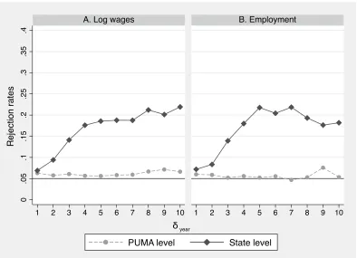
In Figure 1, we first present results with randomly allocated treatment across PUMAs for δ ∈ {1,2, ...,10}. In this case, based on the results derived by Barrios et al. (2012), the proportion of placebo regressions in which the null is rejected at a 5% significance level test should be around 5%. Rejection rates are close to 5% independently of δ, whether we consider log wages (Figure 1.A) or employment (Figure 1.B) as outcome variables.12
This is consistent with the fact that treatment was randomly assigned across PUMAs.
We also present in Figure1rejection rates for simulations in which treatment was assigned at the state level. In this case, we should expect over-rejection if there is spatial correlation in the error term even after taking into account the state and year fixed effects. When we consider simulations in which pre- and post-treatment periods are consecutive years (that is,
δ = 1), there is only mild over-rejection: 6.9% when log wages is used as outcome variable and 7.2% when employment is used as outcome variable. When we increase the distance
12
between the pre- and post-treatment periods, however, the over-rejection sharply increases, reaching more than 20% in some cases.
These results are in line with the intuition presented in Section 2that group fixed effects should capture most of the spatial correlation if the distance between the pre- and post-treatment years is small. However, when this distance is large, then the group fixed effects will capture less of the spatial correlation, implying in more severe over-rejection.
We also consider simulations using the two-way cluster standard errors proposed by
Cameron et al. (2011), clustering at both the PUMA and the year levels. In this case, we modify the simulations because two-way cluster does not work well with only one pre-treatment period and one post-pre-treatment period. Therefore, we include in each simulation ten years of data, with the placebo treatment starting after the fifth year. When we consider treatment randomly allocated across PUMAs, rejection rates are 6.5% and 7% when the out-come variable is, respectively, log wages and employment. There is a slight over-rejection, possibly from the fact that there are only ten periods. In contrast, when we consider treat-ment randomly allocated across states, rejection rates are 23% and 28%. These simulations confirm the intuition presented in Section 2, that two-way cluster procedures may underes-timate the standard errors because they fail to take into account correlations between ηjt
and ηj′t′, for j =6 j′ and t 6= t′. Note that such correlations will appear whenever there
are common shocks that are serially correlated. We present a Monte Carlo simulation in AppendixA that confirms this intuition.
3.2
Simulations with the CPS
We now present simulations using the CPS data from 1979 to 2018. We select two years and two age groups. We vary the distance between the pre- and post-treatment periods (δyear), and the distance between the two age groups (δage), both ranging from 1 to 15. As
post-treatment for one of the age groups. These simulations mimic a setting in which there is a policy change that affects individuals from a specific cohort, so we can use other cohorts as a control group. In these simulations, we treat a pair (state × age) as a group i, and we estimate the treatment effect using a DID model including time fixed effects and state ×
age fixed effects. We test the null hypothesis of no effect based on standard errors clustered at the state level. Therefore, we implicitly assume that the error term for individuals in different states are independent.
In these simulations, we now have measures of proximity both between the pre- and post-periods (δyear), and between the treated and control groups (δage). Therefore, we are able to
validate, in this example, the intuition presented in Section 2 that correlated shocks should be relatively less important when either (i) treated and control groups are more similar, or (ii) the pre-treatment period is close to the post-treatment period.
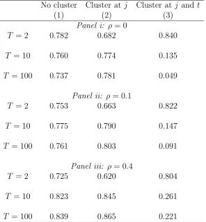
We present in Figure 2rejection rates for combinations of (δyear, δage). Interestingly,
inde-pendently of the outcome variable, rejection rates are generally close to 5% when eitherδyear
or δage is small. For example, even when δyear = 10, in which case the simulations from
Sec-tion 3.1 displayed large over-rejection, rejection rates remain close to 5% when δage is small.
Likewise, rejection rates are still close to 5% when we consider δage = 10, as long as δyear is
small. When both δyear and δage increase, however, we find significant over-rejection. With
(δyear, δage) = (15,15), for example, we find rejection rates of around 37% when we consider
log wages as outcome variable, and 22% for employment. Overall, these simulation results are consistent with the results derived for the linear factor model in Section2, in that spatial correlation only poses important problems for inference when there is both significant differ-ences between the post- and pre-treatment periods (δyear is large) and significant differences
4
Recommendations
Drawing inference in DID models with large N and fixed T is impossible without im-posing restrictions on the variance-covariance matrix of the error. Methods that allow for unrestricted serial correlation essentially collapse the information from the pre- and post-treatment periods, and rely on restrictions in the spatial correlation. Most commonly, it is assumed that errors are independent across groups. Other alternatives would rely on addi-tional information, such as some sort of information on the distance between different groups, or a large number of periods. In many DID applications, however, such distance measures or a large number of periods are not available. Ignoring spatial correlation is, therefore, the only option in many cases.
The results derived in Section 2, and corroborated in simulations with two important datasets in Section 3(the ACS and the CPS), provide guidelines on how one should proceed in empirical applications to minimize the relevance of spatial correlation. We show that spatial correlation can lead to severe over-rejection when (i) the second moment of the difference in the pre- and post-treatment averages of the common factors is large, and (ii) factor loadings have very different distributions for the treated and control groups or factor loadings exhibit spatial correlation.
reliable.13
Moreover, the time periods that are not used in the estimation can be used for placebo exercises. If spatial correlation remains a problem even after restricting the sam-ple to a few periods, then one should expect over-rejection in placebo regressions using the same number of periods, but before the treatment started. This is true even if the parallel trends assumption is valid. Therefore, such placebo exercises will not only provide evidence regarding the validity of the parallel trends assumption, but will also provide evidence for the validity of the inference procedure.
Alternatively, if the focus of the empirical exercise is to estimate the long-term impacts of a policy change, then it would not be possible to minimize E[(¯λpost−λ¯pre)
2
] by restricting the sample to periods around the policy change. Therefore, the effort should be in the direction of guaranteeing that the treated and the control groups are as similar as possible. While, in this case, spatial correlation in the factor loadings could affect inference even if the distribution of factor loadings is the same for treated and control groups, focusing on treated and control groups that are more similar ensures that a larger portion of the spatial correlation is absorbed by the year fixed effects.
5
Conclusion
We analyze the conditions in which correlated shocks pose relevant challenges for infer-ence in DID models. Considering that the spatial correlation structure follows a linear factor model, we analyze the conditions in which (ignored) spatial correlation leads to significant distortions for inference. We present simulations with real datasets that corroborate the conclusions that spatial correlation is less relevant when either the distance between the pre-and post-treatment years is small or the treated pre-and control groups are very similar. The simulation results suggest that the linear factor model analyzed in this paper provides a good approximation to real datasets like the ACS and the CPS. Finally, we provide
recom-13
mendations to minimize the relevance of spatial correlated shocks in DID applications.
References
Adao, R., Kolesar, M., and Morales, E. (2010). Shift-share designs: Theory and inference. Arellano, M. (1987). Computing robust standard errors for within-groups estimators. Oxford
Bulletin of Economics and Statistics, 49(4):431–434.
Athey, S. and Imbens, G. (2018). Design-based Analysis in Difference-In-Differences Settings with Staggered Adoption. Working Paper, arXiv:1808.05293 .
Barrios, T., Diamond, R., Imbens, G. W., and Kolesar, M. (2012). Clustering, spatial correlations, and randomization inference.Journal of the American Statistical Association, 107(498):578–591.
Bertrand, M., Duflo, E., and Mullainathan, S. (2004). How much should we trust differences-in-differences estimates? Quarterly Journal of Economics, page 24975.
Bester, C. A., Conley, T. G., and Hansen, C. B. (2011). Inference with dependent data using cluster covariance estimators. Journal of Econometrics, 165(2):137 – 151.
Brewer, M., Crossley, T. F., and Joyce, R. (2017). Inference with difference-in-differences revisited. Journal of Econometric Methods, 7(1).
Callaway, B. and Sant’Anna, P. H. C. (2018). Difference-in-Differences with Multiple Time Periods and an Application on the Minimum Wage and Employment. Working Paper, arXiv:1803.09015 .
Cameron, A., Gelbach, J., and Miller, D. (2008). Bootstrap-based improvements for inference with clustered errors. The Review of Economics and Statistics, 90(3):414–427.
Cameron, A. C., Gelbach, J. B., and Miller, D. L. (2011). Robust inference with multiway clustering. Journal of Business & Economic Statistics, 29(2):238–249.
Canay, I. A., Romano, J. P., and Shaikh, A. M. (2017). Randomization tests under an approximate symmetry assumption. Econometrica, 85(3):1013–1030.
Conley, T. G. and Taber, C. R. (2011). Inference with Difference in Differences with a Small Number of Policy Changes. The Review of Economics and Statistics, 93(1):113–125. Dailey, A. (2017). Randomization inference with rainfall data: Using historical weather
patterns for variance estimation. Political Analysis, 25(3):277 – 288.
Ferman, B. and Pinto, C. (2019). Inference in differences-in-differences with few treated groups and heteroskedasticity. The Review of Economics and Statistics, 0(ja):null.
Goodman-Bacon, A. (2018). Difference-in-differences with variation in treatment timing. Working Paper 25018, National Bureau of Economic Research.
Kim, M. S. and Sun, Y. (2013). Heteroskedasticity and spatiotemporal dependence robust inference for linear panel models with fixed effects. Journal of Econometrics, 177(1):85 – 108.
MacKinnon, J. G., Nielsen, M., and Webb, M. D. (2019). Wild Bootstrap and Asymp-totic Inference with Multiway Clustering. Working Paper 1415, Economics Department, Queen’s University.
MacKinnon, J. G. and Webb, M. D. (2017). Wild bootstrap inference for wildly different cluster sizes. Journal of Applied Econometrics, 32(2):233–254.
MacKinnon, J. G. and Webb, M. D. (2019). Randomization Inference for Difference-in-Differences with Few Treated Clusters. Journal of Econometrics, Forthcoming.
Menzel, K. (2017). Bootstrap with Clustering in Two or More Dimensions. arXiv e-prints, page arXiv:1703.03043.
Ruggles, S., Genadek, K., Goeken, R., Grover, J., and Sobek, M. (2015). Integrated Public Use Microdata Series: Version 6.0 [Machine-readable database].
Thompson, S. B. (2011). Simple formulas for standard errors that cluster by both firm and time. Journal of Financial Economics, 99(1):1 – 10.
Figure 1: Simulations with the ACS
0
.05
.1
.15
.2
.25
.3
.35
.4
1 2 3 4 5 6 7 8 9 10 1 2 3 4 5 6 7 8 9 10
A. Log wages B. Employment
PUMA level State level
R
e
je
ct
io
n
ra
te
s
δ
year
Notes: This figure presents rejection rates for the simulations using ACS data, presented in Section
3.1. Each simulation has two states and two periods. We considered all combination of pairs of
states and years. The distance between the pre- and post-treatment periods (δyear) varies from
1 to 10 years. The pre-treatment period ranges from 2005 to 2017-δyear. In the “PUMA level”
Figure 2: Simulations with the CPS 1 2 3 4 5 6 7 8 9 10 11 12 13 14 15
1 2 3 4 5 6 7 8 9 101112131415 1 2 3 4 5 6 7 8 9 101112131415 A. Log wages B. Employment
.04 .06 .08 .1 .12 .14 .16 .18 .2 .22 .24 .26 .28 .3 .32 .34 .36 .38 R e je ct io n ra te s
δ age
δ year
Notes: This figure presents rejection rates for the simulations using CPS data, presented in Section
3.2. We considered all combination of pairs of years and pairs of ages. The initial time period
ranges from 1979 to 2018-δyear. The initial age ranges from 25 to 50-δyear. For each simulation, we
A
Monte Carlo Simulations - Two-way Cluster
We present here a small Monte Carlo (MC) simulation to analyze the properties of the two-way cluster in a DID setting. We consider a simple example with 100 groups, half treated and half control, in which Yjt =λ1t+ǫjt whenj ∈ T1 andYjt =λ0t+ǫjt whenj ∈ T0. We set
ǫjt ∼N(0,1), i.i.d. across both j and t. We also set E[λwt] = 0 for w∈ {0,1} and for all t,
so the DID estimator is unbiased. However, the λw
t generates important spatial correlation
that is not absorbed by the time fixed effects. The λw
t follows an AR(ρ) process, withρ ∈ {0,0.1,0.4}. We also setT ∈ {2,10,100}. In
all simulations, treatment starts after period T /2. Appendix Table 1present rejection rates based on (i) robust standard errors (with no cluster), (ii) standard errors clustered at group level, and (iii) standard errors clustered at two levels, group and time. As expected, there is a severe over-rejection when we consider inference without clustering, or clustering only at the group level. This happens because this data generating process includes substantial spatial correlation, that is not captured in these variance estimators.
With T = 2, using a two-way cluster — at the time and group levels — does not solve the problem. The limitation of the two-way cluster estimator in this case comes from the fact that there is only one post-treatment period and one pre-treatment period. When
ρ= 0, rejection rates converge to 5% when T increases. Whenρ >0, however, there is still over-rejection even when T is large. Moreover, the over-rejection is increasing withρ.
These results confirm the intuition presented in Section2, that two-way cluster procedures may underestimate the standard errors, because they fail to take into account correlations betweenηjt andηj′t′, for j 6=j′ and t6=t′. Note that the only case in which such correlation
Table 1: Monte Carlo Simulations - Two-way Cluster
No cluster Cluster atj Cluster at j and t
(1) (2) (3)
Panel i: ρ = 0
T = 2 0.782 0.682 0.840
T = 10 0.760 0.774 0.135
T = 100 0.737 0.781 0.049
Panel ii: ρ= 0.1
T = 2 0.753 0.663 0.822
T = 10 0.775 0.790 0.147
T = 100 0.761 0.803 0.091
Panel iii: ρ= 0.4
T = 2 0.725 0.620 0.804
T = 10 0.823 0.845 0.261
T = 100 0.839 0.865 0.221
Notes: This table presents rejection rates for the simulations described in Appendix A. Column