http://www.scirp.org/journal/jamp ISSN Online: 2327-4379
ISSN Print: 2327-4352
DOI: 10.4236/jamp.2017.510171 Oct. 31, 2017 2051 Journal of Applied Mathematics and Physics
Computation of the Eigenvalues of 3D
“Charged” Integral Equations
Diego Caratelli
1,2, Pierpaolo Natalini
3, Paolo E. Ricci
41The Antenna Company, High Tech Campus, Eindhoven, the Netherlands 2Tomsk Polytechnic University, Tomsk, Russia
3Università degli Studi Roma Tre, Largo San Leonardo Murialdo, Roma, Italia
4International Telematic University UniNettuno, Corso Vittorio Emanuele II, Roma, Italia
Abstract
The Rayleigh-Ritz and the inverse iteration methods are used in order to compute the eigenvalues of 3D Fredholm-Stieltjes integral equations, i.e. 3D
Fredholm equations with respect to suitable Stieltjes-type measures. Some ap-plications are shown, relevant to the problem of computing the eigenvalues of a body charged by a finite number of masses concentrated on points, curves or surfaces lying in.
Keywords
3D Fredholm-Stieltjes Integral Equations, Eigenvalues, Rayleigh-Ritz Method, Inverse Iteration Method
1. Introduction
The theory of Fredholm integral equations is strictly connected with the birth of functional analysis. A background of this theory can be found in classical books (see e.g. [1] [2]). For recent developments relevant to numerical computation of solutions, see [3].
In [4] [5], the Author shows that the Fredholm theory still holds considering the so called charged Fredholm integral equations, i.e. Fredholm equations with respect to a Stieltjes measure obtained by adding to the ordinary Lebesgue measure a finite combination of positive masses concentrated in arbitrary points of the considered interval. A topic which at present is included, as a particular case, in the theory of strictly positive compact operators.
In the one-dimensional case, the mechanical interpretation of these equations
How to cite this paper: Caratelli, D., Na-talini, P. and Ricci, P.E. (2017) Computa-tion of the Eigenvalues of 3D “Charged” Integral Equations. Journal of Applied Mathematics and Physics, 5, 2051-2071. https://doi.org/10.4236/jamp.2017.510171 Received: October 7, 2017
Accepted: October 28, 2017 Published: October 31, 2017 Copyright © 2017 by authors and Scientific Research Publishing Inc. This work is licensed under the Creative Commons Attribution International License (CC BY 4.0).
DOI: 10.4236/jamp.2017.510171 2052 Journal of Applied Mathematics and Physics
is connected with the problem of the free vibrations of a string charged by a finite number of cursors, and is related to an extension of the classical orthogonality property of eigensolutions, called the “Sobolev-type” orthogonality (see e.g. [6] [7]).
In preceding articles [8] [9] [10], the problem of numerical computation of the above mentioned eigenvalue problems was solved, by using the so called inverse iteration method, showing applications in one and two-dimensional cases.
In this article, after briefly recalling the main results about the theory of eigenvalues for charged Fredholm integral equations, we mention how to obtain (in the particular case of a symmetric and strictly positive operator), the lower and upper approximations of these eigenvalues by means of the Rayleigh-Ritz method [1], [11] and the Fichera orthogonal invariants method [11] [12]
respectively. Then we conclude by showing that, even in the three-dimensional case, the lower approximations of the eigenvalues obtained by means of the Rayleigh-Ritz method can be improved by applying the inverse iteration method
[13]. Numerical computations relevant to the considered case are developed in the concluding section.
2. Lebesgue-Stieltjes Measures in a 3D Interval
Consider the interval and the Hilbert space 2 2
( )
dM dM
L
≡
L
equipped withthe scalar product
[
,]
:(
,)
( )(
,)
(
,)
(
,)
r n m
P dP dM
U V U V ρ U V U V γ U V
Σ
∆ ∆ ∆
= + + + (1)
where
[
,]
(
,)
2dM
L dM
U V ≡ U V and the subscripts “ρ
( )
P dP”, “∆r”, “∆γn”, “m
Σ
∆ ”
refer to the following definitions:
(
U V,)
ρ( )P dP:=∫
U P V P( ) ( ) ( )
ρ P dP (2)
(
)
( ) ( )
1
, :
r
r
h h h h
U V ∆ m U A V A
=
=
∑
(3)(
)
(
( )
)
(
( )
)
(
( )
)
1
, : d
n k
n
k k
U V ∆γ γσ P s U P s V P s s
=
=
∑∫
(4)and
(
)
(
( )
)
(
( )
)
(
( )
)
1
, : , , , d
m
m
U V τ P u v U P u v V P u v σ
Σ
∆ =
∑∫
= Σ , (5)
(obviously 2
d :
σ
= EG−F d du v), so that the Stieltjes measure is the sum of theordinary Lebesgue measure plus a finite sum of charges mh concentrated on
points Ah⊂ ,
(
h=1, 2,,r)
, plus a finite sum of continuous chargesbelonging to the curves Σ ⊂ , with densities σk
( )
⋅ ,(
k=1, 2,,n)
, plus afinite sum of continuous charges belonging to the surfaces Σ ⊂ , with densities τk
( )
⋅ ,(
=1, 2,,m)
.It is worth noting that 2
( )
dMDOI: 10.4236/jamp.2017.510171 2053 Journal of Applied Mathematics and Physics
space 2
( )
L
, a (complete) Hilbert space, which does not have singularities (i.e.discontinuities) at points Ah,
(
h=1, 2,,r)
, at curves γk,(
k=1, 2,,n)
,and surfaces Σ,
(
=1, 2,,m)
, according to the usual condition for existenceof the relevant Stieltjes integrals (see e.g. [14]).
Let us consider, for example, the computation of integrals with respect to the above Dirac-type measures:
(
,) ( )
h( )
h h(
, h) ( )
hK P Q ϕ Q mδ A =m K P A ϕ A
∫
(
) ( )
(
( )
)
(
( )
)
( )
(
)
(
( )
)
(
( )
)
, d , d k k kK P Q Q Q s Q s s
K P Q s Q s Q s s
γ γ
ϕ
σ
δ
ϕ
τ
=∫
∫
∫
(
) ( )
(
( )
)
(
( )
)
( )
(
)
(
( )
)
(
( )
)
, , , d
, , , , d
K P Q Q Q u v Q u v
K P Q u v Q u v Q u v
ϕ
τ
δ
σ
ϕ
τ
σ
Σ Σ =
∫
∫
∫
These formulas will be useful in the following.
The Eigenvalue Problem for 3D “Charged” Operators
Consider in 2
( )
dML
the eigenvalue problem ϕ µϕ= (6)
( )
: K( ) ( )
,Q Q dMQ ϕ ⋅ =∫
⋅ ϕ (7)
where K P Q
(
,)
is a symmetric kernel, and( )
( )
(
( )
)
(
( )
)
( )
(
)
(
( )
)
1 1
1
d d d
, , d
k
r n
Q h h k
h k
m
M Q Q m A Q s Q s s
Q u v Q u v
γ
ρ δ σ δ
τ δ σ
= = Σ = = + + +
∑
∑∫
∑∫
(8)(δ denoting the usual Dirac-Delta function). According to the above positions, we have
( )( )
(
) ( ) ( )
(
) ( )
(
)
(
( )
)
(
( )
)
(
( )
)
(
)
(
( )
)
(
( )
)
(
( )
)
(
) ( )
(
)
( )(
(
) ( )
)
( )(
) ( )
(
)
( )(
(
) ( )
)
( ) 1 1 1, d ,
, d
, , , d
, , , , , , , , k r n m r
h h h
h n
k k
m
Q dQ Q
Q Q
P K P Q Q Q Q m K P A A
K P Q Q s Q s Q s s
K P Q Q s Q u v Q u v
K P Q Q K P Q Q
K P Q Q K P Q Q
γ
ρ γ
ϕ ϕ ρ ϕ
ϕ σ δ
ϕ τ δ σ
ϕ ϕ ϕ ϕ Σ = = Σ = ∆ ∆ ∆ = + + + = + + +
∑
∫
∑∫ ∫
∑∫ ∫
(9) so that[
]
(
(
)( ) ( )
)
( )(
(
)( ) ( )
)
( )(
)( ) ( )
(
)
( ) , , , , r ndM P dP P
P
U V U P V P U P V P
U P V P
γ ρ ∆ ∆ = + +
DOI: 10.4236/jamp.2017.510171 2054 Journal of Applied Mathematics and Physics
[
]
(
) ( )
(
)
( )( )
(
)
( )(
(
(
) ( )
)
( )( )
)
( )(
) ( )
(
)
( )( )
(
)
( )(
(
(
) ( )
)
( )( )
)
( )(
) ( )
(
)
( )( )
(
)
( )(
(
(
) ( )
)
( )( )
)
( )(
) ( )
(
)
( )( )
(
)
( )(
(
(
) ( )
)
( )( )
)
( ) , , , , , , , , , , , , , , , , , , , , , , , , , r n m r r rn r m r
dM
Q dQ Q
P dP P dP
Q Q
P dP P dP
Q dQ Q
P P
Q Q
P P
U V
K P Q U Q V P K P Q U Q V P
K P Q U Q V P K P Q U Q V P
K P Q U Q V P K P Q U Q V P
K P Q U Q V P K P Q U Q V P
ρ ρ ρ
γ ρ ρ
ρ γ Σ Σ ∆ ∆ ∆ ∆ ∆ ∆ ∆ ∆ ∆ ∆ = + + + + + + +
(
) ( )
(
)
( )( )
(
)
( )(
(
(
) ( )
)
( )( )
)
( )(
) ( )
(
)
( )( )
(
)
( )(
(
(
) ( )
)
( )( )
)
( )(
) ( )
(
)
( )( )
(
)
( )(
(
(
) ( )
)
( )( )
)
( )(
) ( )
(
)
( )( )
(
)
( )(
(
(
) ( )
)
( )( )
)
( ) , , , , , , , , , , , , , , , , , , , , , , , , r n nn n m n
r
m m
n m
m m
Q dQ Q
P P
Q Q
P P
Q dQ Q
P P
Q P Q
P
K P Q U Q V P K P Q U Q V P
K P Q U Q V P K P Q U Q V P
K P Q U Q V P K P Q U Q V P
K P Q U Q V P K P Q U Q V P
ρ γ γ
γ γ γ
ρ γ Σ Σ Σ Σ Σ Σ ∆ ∆ ∆ ∆ ∆ ∆ ∆ ∆ ∆ ∆ ∆ ∆ ∆ ∆ + + + + + + + + Furthermore
(
) ( )
(
)
( )( )
(
)
( )(
) ( ) ( ) ( ) ( )
, , ,, d d
Q dQ
P dP
K P Q U Q V P
K P Q U Q V P P Q P Q
ρ ρ ρ ρ × =
∫∫
(
) ( )
(
)
( )( )
(
)
( )( )
(
) ( ) ( )
1 , , , , drQ P dP
r
h h h
h
K P Q U Q V P
m U A K P A V P P P
ρ ρ ∆ = =
∑
∫
(
) ( )
(
)
( )( )
(
)
( )( )
(
) ( ) ( )
1 , , , , d rQ dQ P
r
h h h
h
K P Q U Q V P
m V A K P A U P P P
ρ ρ ∆ = =
∑
∫
where we used the symmetry of the kernel,
(
) ( )
(
)
( )( )
(
)
( )( )
(
)
(
( )
)
(
( )
)
( ) ( )
1 , , ,, d d
n
k
Q P dP
n
k
K P Q U Q V P
K P Q s U Q s Q s V P P s P
γ ρ
γ τ ρ
∆ = =
∑∫ ∫
(
) ( )
(
)
( )( )
(
)
( )( )
(
)
(
( )
)
(
( )
)
( ) ( )
1 , , ,, d d
n k Q dQ P n k k
K P Q U Q V P
K P Q s V Q s Q s U P P s P
ρ γ
γ σ ρ
∆ = =
∑∫ ∫
(
) ( )
(
)
( )( )
(
)
( )(
( ) ( )
)
(
( )
)
( )
(
)
(
( )
)
(
( )
)
1 1 1 2 , , , , , , ,, , , d d
j m m m m Q P j
K P Q U Q V P K P t w Q u v U Q u v
V P t w τ Q u v τ P t w σ σ
Σ
Σ
∆ ∆ Σ Σ
= = = ×
∑∑∫ ∫
DOI: 10.4236/jamp.2017.510171 2055 Journal of Applied Mathematics and Physics
(
) ( )
(
)
( )( )
(
)
( )( )
(
)
(
( )
)
(
( )
)
( ) ( )
1 , , ,, , , , d d
m Q P dP
m
K P Q U Q V P
K P Q u v U Q u v Q u v V P P P
ρ
τ ρ σ
Σ ∆ Σ = =
∑∫ ∫
(
) ( )
(
)
( )( )
(
)
( )( )
(
)
(
( )
)
(
( )
)
( ) ( )
1 , , ,, , , , d d
m
Q dQ
P
m
K P Q U Q V P
K P Q u v V Q u v Q u v U P P P
ρ
τ ρ σ
Σ ∆ Σ = =
∑∫ ∫
where we used the symmetry of the kernel,
(
) ( )
(
)
( )( )
(
)
( )(
)
( )
( )
1 1 , , , , r r Q P r rh j h j h j
h j
K P Q U Q V P
m m K A A U A V A
∆ ∆ = = =
∑∑
(
) ( )
(
)
( )( )
(
)
( )( )
(
( )
)
(
( )
)
(
( )
)
1 1 , , , , d n r k Q P r nh h h k
h k
K P Q U Q V P
m V A K A Q s U Q s Q s s
γ γ σ ∆ ∆ = = =
∑
∑∫
(
) ( )
(
)
( )( )
(
)
( )( )
(
( )
)
(
( )
)
(
( )
)
1 1 , , , , d r n k Q P r nh h h k
h k
K P Q U Q V P
m U A K A Q s V Q s Q s s
γ
γ σ
∆ ∆
= =
=
∑
∑∫
where we used the symmetry of the kernel,
(
) ( )
(
)
( )( )
(
)
( )( )
(
( )
)
(
( )
)
(
( )
)
1 1 , , ,, , , , d
mQ rP
r m
h h h
h
K P Q U Q V P
m V A K A Q u v U Q u v τ Q u v σ
Σ ∆ ∆ Σ = = =
∑
∑∫
(
) ( )
(
)
( )( )
(
)
( )( )
(
( )
)
(
( )
)
(
( )
)
1 1 , , ,, , , , d
r
m
Q
P
r m
h h h
h
K P Q U Q V P
m U A K A Q u v V Q u v τ Q u v σ
Σ ∆ ∆ Σ = = =
∑
∑∫
where we used the symmetry of the kernel,
(
) ( )
(
)
( )( )
(
)
( )( )
(
)
(
( )
)
(
( ) ( )
)
(
( )
)
(
( )
)
1 1 , , ,, , , , d d
m n Q P n m k k
K P Q U Q V P
V P s P s K P s Q u v U Q u v Q u v s
γ
σ τ σ
Σ ∆ ∆ Σ = = =
∑
∑∫
(
) ( )
(
)
( )( )
(
)
( )( )
(
)
(
( )
)
(
( ) ( )
)
(
( )
)
(
( )
)
1 1 , , ,, , , , d d
n m Q P n m k k
K P Q U Q V P
U P s P s K P s Q u v V Q u v Q u v s
γ
σ τ σ
Σ ∆ ∆ Σ = = =
∑
∑∫
DOI: 10.4236/jamp.2017.510171 2056 Journal of Applied Mathematics and Physics
(
) ( )
(
)
( )( )
(
)
( )( ) ( )
(
)
(
( )
)
(
( )
)
(
( )
)
(
( )
)
1 1 , , ,, d d
n n k Q P n n k k
K P Q U Q V P
K P Q s U Q s V P Q s P s
γ γ
γ γ σ σ σ σ σ σ
∆ ∆ = = =
∑∑∫ ∫
(
) ( )
(
)
( )( )
(
)
( )( ) ( )
(
)
(
( )
)
( )
(
)
(
( )
)
(
( )
)
1 1 1 2 , , , , , , ,, , , d d
m m j Q P m m j
K P Q U Q V P
K P t w Q u v U Q u v
V P t w τ Q u v τ P t w σ σ
Σ Σ ∆ ∆ Σ Σ = = = ×
∑∑∫ ∫
3. Computation of the Eigenvalues for Charged
Integral Equations
The computation of the eigenvalues of second kind Fredholm integral equations is usually performed by using the Rayleig-Ritz method [1] [11] for lower bounds, and the Fichera orthogonal invariants method [11] [12] for upper bounds. An alternative procedure, called the inverse iteration method, can be used to improve the lower approximations previously obtained by means of the Rayleigh-Ritz method. This approach was already considered in [13], and will be applied even in the present case.
We will not describe herewith the three above mentioned methods, because they are essentially independent of the dimension of the considered vibrating item (string, membrane or body). We refer for shortness to the above mentioned articles [8] [9] [11] [12].
4. Applications
Let ≡
[ ] [ ] [ ]
0,a × 0,b × 0,c , O≡(
0, 0, 0 ,)
U≡(
a b c, ,)
,(
P, P, P)
,(
Q, Q, Q)
,(
P, P, Q)
,(
P, Q, Q)
P≡ x y z Q≡ x y z R≡ x y z S≡ x y z
(
Q, P, P)
,(
Q, Q, P)
,(
P, Q, P)
,(
Q, P, Q)
T ≡ x y z L≡ x y z M ≡ x y z N≡ x y z
0≤xP≤a, 0≤yP≤b, 0≤zP≤c
0≤xQ≤a, 0≤yQ≤b, 0≤zQ≤c
(
)
, if , , ,
, if , , ,
, if , , ,
, if , , ,
,
, if , , ,
, if , , ,
, if , , ,
, if
P Q P Q P Q
P Q P Q P Q
P Q P Q P Q
P Q P Q P Q
P Q P Q P Q
P Q P Q P Q
P Q P Q P Q
P Q
OP UQ x x y y z z
OQ UP x x y y z z
OR UL x x y y z z
OS UT x x y y z z
K P Q
OT US x x y y z z
OL UR x x y y z z
OM UN x x y y z z
ON UM x x
⋅ ≤ ≤ ≤ ⋅ ≥ ≥ ≥ ⋅ ≤ ≤ ≥ ⋅ ≤ ≥ ≥ = ⋅ ≥ ≤ ≤ ⋅ ≥ ≥ ≤ ⋅ ≤ ≥ ≤
DOI: 10.4236/jamp.2017.510171 2057 Journal of Applied Mathematics and Physics
(
)
(
) (
) (
)
(
) (
) (
)
(
) (
)
(
)
(
)
(
) (
)
2 2 2
2 2 2
2 2 2
2 2 2
2 2 2
2 2 2
2 2 2
2 2 2
, if , , ,
, if , , ,
, if , , ,
, if , ,
,
P P P Q Q Q P Q P Q P Q
Q Q Q P P P P Q P Q P Q
P P Q Q Q P P Q P Q P Q
P Q Q Q P P P Q P Q P Q
x y z a x b y c z x x y y z z
x y z a x b y c z x x y y z z
x y z a x b y c z x x y y z z
x y z a x b y c z x x y y z z
K P Q
+ + − + − + − ≤ ≤ ≤ + + − + − + − ≥ ≥ ≥ + + − + − + − ≤ ≤ ≥ + + − + − + − ≤ ≥ ≥ =
(
)
(
) (
)
(
) (
)
(
)
(
)
(
)
(
)
(
)
(
)
(
)
2 2 22 2 2
2
2 2
2 2 2
2 2 2
2 2 2
2
2 2
2 2 2
,
, if , , ,
, if , , ,
, if , , ,
, if , , .
Q P P P Q Q P Q P Q P Q
Q Q P P P Q P Q P Q P Q
P Q P Q P Q P Q P Q P Q
Q P Q P Q P P Q P Q P Q
x y z a x b y c z x x y y z z
x y z a x b y c z x x y y z z
x y z a x b y c z x x y y z z
x y z a x b y c z x x y y z z
+ + − + − + − ≥ ≤ ≤ + + − + − + − ≥ ≥ ≤ + + − + − + − ≤ ≥ ≤ + + − + − + − ≥ ≤ ≥
Obviously K P Q
(
,)
=K Q P(
,)
, i.e. the kernel is symmetric, and even positive definite, since K P Q(
,)
>0, ∀(
P Q,)
∈.Consider in 2
( )
dML
the eigenvalue problem ϕ µϕ= (2)
( ) ( )
: K ,Q Q dMQϕ =
∫
⋅ ϕ
(3)
where
( )
( )
(
( )
)
(
( )
)
( )
(
)
(
( )
)
1 1 1d d d
, , d
k
r n
Q h h k
h k
m
M Q Q m A Q s Q s s
Q u v Q u v
γ
ρ δ σ δ
τ δ σ
= = Σ = = + + +
∑
∑∫
∑∫
(δ denoting the usual Dirac-Delta function).
The considered operator is compact and strictly positive, since it is connected with free vibrations of a body charged by a finite number of masses concentrated on points, curves, or surfaces contained in .
Numerical Example 1
Let a= = =b c 1, and dM =ρ
(
x y z, ,)
d d dx y z with(
x y z, ,)
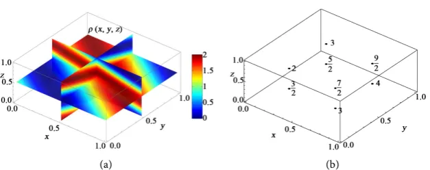
1 2x 3y 4zρ = + + + (see Figure 1). Under this assumption, the
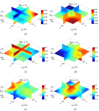
apprpximate eigenvalues evaluated by using the Rayleigh-Ritz and inverse iteration methods are listed in Table 1, whereas the relevant eigenfunctions are shown in Figure 2.
Numerical Example 2
Let a= = =b c 1, and dM =ρ
(
x y z, ,)
d d dx y z with(
)
( )2(
)
3
, , 8π e x y z sin π
x y z xyz
ρ = − + +
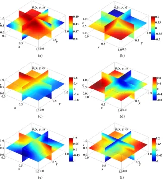
(see Figure 3). Under this assumption, the approximate eigenvalues evaluated by using the Rayleigh-Ritz and inverse iteration methods are listed in Table 2, whereas the relevant eigenfunctions are shown in Figure 4.
DOI: 10.4236/jamp.2017.510171 2058 Journal of Applied Mathematics and Physics
Figure 1. Spatial distribution of the volume density function ρ
(
x y z, ,)
relevant to the numerical Example 1.(a) (b)
(c) (d)
(e) (f)
DOI: 10.4236/jamp.2017.510171 2059 Journal of Applied Mathematics and Physics
Figure 3. Spatial distribution of the volume density function ρ
(
x y z, ,)
relevant to the numerical Example 2.(a) (b)
(c) (d)
(e) (f)
[image:9.595.208.538.322.686.2]DOI: 10.4236/jamp.2017.510171 2060 Journal of Applied Mathematics and Physics
Table 1. Approximate eigenvalues µh and µˆh (h=1, 2,, 6) relevant to the numerical Example 1, as computed by means of the Rayleigh-Ritz and inverse iteration method, respectively.
h µh µˆh
1 2.30919 2.30934
2 0.584150 0.584855
3 0.580232 0.580932
4 0.144731 0.145178
5 0.136953 0.137599
6 0.135077 0.135689
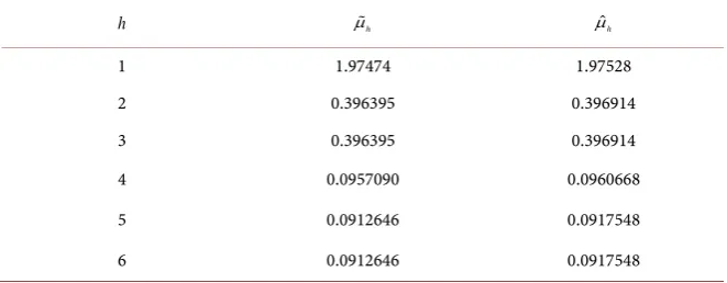
Table 2. Approximate eigenvalues µh and µˆh (h=1, 2,, 6) relevant to the numerical Example 2, as computed by means of the Rayleigh-Ritz and inverse iteration method, respectively.
h µh µˆh
1 1.97474 1.97528
2 0.396395 0.396914
3 0.396395 0.396914
4 0.0957090 0.0960668
5 0.0912646 0.0917548
6 0.0912646 0.0917548
(
)
1 1 1d , , d d d d d d
2 2 2
M =ρ x y z x y z+δx− δ y− δ z− x y z
with
ρ
(
x y z
, ,
)
=
e
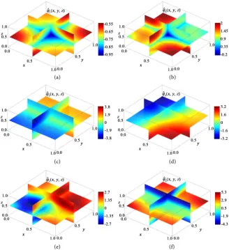
− − −x y z (see Figure 5). Under this assumption, theapproximate eigenvalues evaluated by using the Rayleigh-Ritz and inverse iteration methods are listed in Table 3, whereas the relevant eigenfunctions are shown in Figure 6.
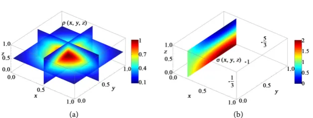
Numerical Example 4 Let a= = =b c 1, and
(
)
(
) (
) (
)
d , , d d d h h h h d d d
h
M =ρ x y z x y z+
∑
mδ x−x δ y−y δ z−z x y z with(
x y z, ,)
2 log 1(
z(
1 y(
1 x)
)
)
ρ = + + + , and mh=1
(
xh+yh+zh)
,1 1
2
h h h
x y z h
H
= = = −
for h=1, 2, 3=H (see Figure 7). Under this assump-
tion, the approximate eigenvalues evaluated by using the Rayleigh-Ritz and inverse iteration methods are listed in Table 4, whereas the relevant eigenfunctions are shown in Figure 8.
Numerical Example 5 Let a= = =b c 1, and
(
)
(
) (
) (
)
d , , d d d h h h h d d d
h
[image:10.595.209.540.301.430.2]DOI: 10.4236/jamp.2017.510171 2061 Journal of Applied Mathematics and Physics
[image:11.595.225.528.62.180.2] [image:11.595.209.538.228.588.2]
(a) (b)
Figure 5. Spatial distribution of the volume density ρ
(
x y z, ,)
(a) and concentrated density functions (b) relevant to the numerical Example 3.(a) (b)
(c) (d)
[image:11.595.205.537.640.734.2](e) (f)
Figure 6. Spatial distribution of the approximate eigenfunctions ϕˆh
(
x y z, ,)
(h=1, 2,, 6) relevant to the numerical Example 3.(
, ,)
1 cos π(
1 2 3 4)
2
x y z x y z
ρ = + − − −
, and mh =3xh+2yh+zh,
1 2 5 6 1 3 5 7 1 2 3 4
1 4
x =x =x =x =y =y =y =y = =z z =z =z = ,
3 4 7 8 2 4 6 8 5 6 7 8
3 4
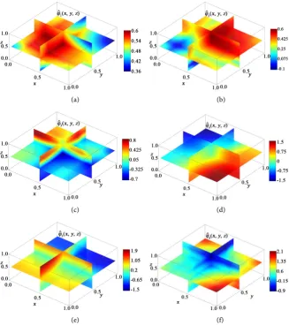
DOI: 10.4236/jamp.2017.510171 2062 Journal of Applied Mathematics and Physics (a) (b)
Figure 7. Spatial distribution of the volume density ρ
(
x y z, ,)
(a) and concentrated density functions (b) relevant to the numerical Example 4.(a) (b)
(c) (d)
(e) (f)
Figure 8. Spatial distribution of the approximate eigenfunctions ϕˆh
(
x y z, ,)
(h=1, 2,, 6) relevant to the numerical Example 4.(see Figure 9). Under this assumption, the approximate eigenvalues evaluated by using the Rayleigh-Ritz and inverse iteration methods are listed in Table 5, whereas the relevant eigenfunctions are shown in Figure 10.
[image:12.595.210.538.245.614.2]DOI: 10.4236/jamp.2017.510171 2063 Journal of Applied Mathematics and Physics
[image:13.595.218.532.66.190.2]
(a) (b)
[image:13.595.211.538.286.393.2]Figure 9. Spatial distribution of the volume density ρ
(
x y z, ,)
(a) and concentrated density functions (b) relevant to the numerical Example 5.Table 3. Approximate eigenvalues µh and µˆh (h=1, 2,, 6) relevant to the numerical Example 3, as computed by means of the Rayleigh-Ritz and inverse iteration method, respectively.
h µh µˆh
1 0.827191 0.827079
2 0.0286952 0.0287715
3 0.0258541 0.0258874
4 0.0258541 0.0258874
5 0.0071926 0.00721217
6 0.00628217 0.00631337
Table 4. Approximate eigenvalues µh and µˆh (h=1, 2,, 6) relevant to the numerical Example 2, as computed by means of the Rayleigh-Ritz and inverse iteration method, respectively.
h µh µˆh
1 1.37202 1.38514
2 0.461313 0.439849
3 0.150812 0.148043
4 0.122611 0.121926
5 0.115747 0.115269
6 0.0456381 0.0440725
Table 5. Approximate eigenvalues µh and µˆh (h=1, 2,, 6) relevant to the numerical Example 5, as computed by means of the Rayleigh-Ritz and inverse iteration method, respectively.
h µh µˆh
1 11.6841 12.0167
2 3.25662 3.10980
3 3.18704 3.04593
4 1.27341 1.30780
5 0.211891 0.195245
[image:13.595.211.538.453.559.2] [image:13.595.210.539.618.734.2]DOI: 10.4236/jamp.2017.510171 2064 Journal of Applied Mathematics and Physics (a) (b)
(c) (d)
[image:14.595.209.540.64.438.2](e) (f)
Figure 10. Spatial distribution of the approximate eigenfunctions ϕˆh
(
x y z, ,)
(h=1, 2,, 6) relevant to the numerical Example 5.Let a= = =b c 1, and
(
)
(
) (
)
(
) (
) (
)
d , , d d d , , d d d
d d d s
h h h
h
M x y z x y z x y z z x y z
x x y y z z x y z
ρ
σ
δ
ζ
δ
δ
δ
= + −
+
∑
− − −with
ρ
(
x y z, ,)
=cosh 2(
y− +x)
sin 2(
x−y)
(
1 e+ x y+)
,σ
(
x y z
, ,
)
=
e
− − +2x3y4z, 14 s
ζ = , and 1 1 1
2
h h
x y h
H
= − = −
,
4 5 h
z = for h=1, 2=H (see Figure 11).
Under this assumption, the approximate eigenvalues evaluated by using the Rayleigh-Ritz and inverse iteration methods are listed in Table 6, whereas the relevant eigenfunctions are shown in Figure 12.
Numerical Example 7
Let a= = =b c 1 , and
(
)
(
) (
)
(
) (
) (
)
d , , d d d , , d d d
d d d s
h h h h
h
M x y z x y z x y z x x y z
m x x y y z z x y z
ρ
σ
δ
ξ
δ
δ
δ
= + −
+
∑
− − −with
(
)
(
) (
2) (
2)
2 1 2, , sech 4 1 2 1 2 1 2
x y z x y z
ρ = − + − + −
,
(
x y z, ,)
5x sin 2( ) ( )
y cos 3zσ = + , 1
5 s
ξ = , and mh=yh+zh, 3 4 h
DOI: 10.4236/jamp.2017.510171 2065 Journal of Applied Mathematics and Physics (a) (b)
Figure 11. Spatial distribution of the volume density ρ
(
x y z, ,)
(a) and concentrated density functions (b) relevant to the numerical Example 6.(a) (b)
(c) (d)
(e) (f)
Figure 12. Spatial distribution of the approximate eigenfunctions ϕˆh
(
x y z, ,)
(h=1, 2,, 6) relevant to the numerical Example 6.1 1
2
h h
y z h
H
= = −
for h=1, 2, 3=H (see Figure 13). Under this assumption,
[image:15.595.210.539.235.602.2]DOI: 10.4236/jamp.2017.510171 2066 Journal of Applied Mathematics and Physics
[image:16.595.217.532.61.180.2] [image:16.595.210.537.228.591.2]
(a) (b)
Figure 13. Spatial distribution of the volume density ρ
(
x y z, ,)
(a) and concentrated density functions (b) relevant to the numerical Example 7.(a) (b)
(c) (d)
(e) (f)
Figure 14. Spatial distribution of the approximate eigenfunctions ϕˆh
(
x y z, ,)
(h=1, 2,, 6) relevant to the numerical Example 7.Numerical Example 8 Let a= = =b c 1, and
(
)
( )
(
( )
)
(
d , , d d d , , d d d
3 3 3
d d d
4 4 4
s
M x y z x y z x y z x y x y z
x y z x y z
ρ σ δ ζ
δ δ δ
= + −
+ − − −
DOI: 10.4236/jamp.2017.510171 2067 Journal of Applied Mathematics and Physics
Table 6. Approximate eigenvalues µh and µˆh (h=1, 2,, 6) relevant to the numerical Example 6, as computed by means of the Rayleigh-Ritz and inverse iteration method, respectively.
h µh µˆh
1 1.46677 1.48646
2 0.636561 0.607952
3 0.142093 0.142025
4 0.0434152 0.0451649
5 0.0287695 0.0298745
6 0.0179072 0.0179560
Table 7. Approximate eigenvalues µh and µˆh (h=1, 2,, 6) relevant to the numerical Example 7, as computed by means of the Rayleigh-Ritz and inverse iteration method, respectively.
h µh µˆh
1 1.71928 1.75065
2 0.404514 0.391333
3 0.327108 0.328006
4 0.155119 0.152451
5 0.133601 0.132340
6 0.0390550 0.0389560
with
ρ
(
x y z, ,)
=3 2 cos+( )
xz +sin( ) (
yz 1 2+ x+3y+4z)
, and( ) (
x y, 1 2x 3y)
7 cos 6( )
y sin 5( )
xσ
= + + + + ,( )
1( )
( )
, 1 cos sin 3
2
s x y x y
ζ = + − (see Figure 15). Under this assumption, the
approximate eigenvalues evaluated by using the Rayleigh-Ritz and inverse iteration methods are listed in Table 8, whereas the relevant eigenfunctions are shown in Figure 16.
Numerical Example 9 Let a= = =b c 1, and
(
)
( )
(
( )
)
( )
(
( )
)
(
( ))
(
) (
) (
)
d , , d d d , , d d d
d d d
d d d s
l l
h h h h
h
M x y z x y z x y z x y x y z
z x z y z x y z
m x x y y z z x y z
ρ σ δ ζ
τ δ ξ δ η
δ δ δ
= + −
+ − −
+
∑
− − −with ρ
(
x y z, ,)
= +4 3cos 3( )
x +2 sin 2( )
y +tan( )
z , σ(
x y,)
=2 log 1(
+ +y xy)
,( )
1(
)
, 1 2
4
s x y x y
ζ = − + , τ
( )
z =2z, ξl( )
z =ηl( )
z =4z−3, andh h h h
m =x +y +z , 1 2 1 3 1 4
x =x = y =y = , 3 4 2 4 3 4
x =x =y =y = , 2
3 h
[image:17.595.212.539.300.433.2]DOI: 10.4236/jamp.2017.510171 2068 Journal of Applied Mathematics and Physics (a) (b)
Figure 15. Spatial distribution of the volume density ρ
(
x y z, ,)
(a) and concentrated density functions (b) relevant to the numerical Example 8.(a) (b)
(c) (d)
(e) (f)
Figure 16. Spatial distribution of the approximate eigenfunctions ϕˆh
(
x y z, ,)
(h=1, 2,, 6) relevant to the numerical Example 8.1, 2, 3, 4
h= =H (see Figure 17). Under this assumption, the approximate
[image:18.595.211.538.241.629.2]DOI: 10.4236/jamp.2017.510171 2069 Journal of Applied Mathematics and Physics (a) (b)
Figure 17. Spatial distribution of the volume density ρ
(
x y z, ,)
(a) and concentrated density functions (b) relevant to the numerical Example 9.(a) (b)
(c) (d)
(e) (f)
Figure 18. Spatial distribution of the approximate eigenfunctions ϕˆh
(
x y z, ,)
(h=1, 2,, 6) relevant to the numerical Example 9.Acknowledgements
[image:19.595.209.538.244.640.2]DOI: 10.4236/jamp.2017.510171 2070 Journal of Applied Mathematics and Physics
Table 8. Approximate eigenvalues µh and µˆh (h=1, 2,, 6) relevant to the numerical Example 8, as computed by means of the Rayleigh-Ritz and inverse iteration method, respectively.
h µh µˆh
1 1.24996 1.28312
2 0.232580 0.236340
3 0.212298 0.213581
4 0.175619 0.177549
5 0.0535925 0.0541850
6 0.0451690 0.0465835
Table 9. Approximate eigenvalues µh and µˆh (h=1, 2,, 6) relevant to the numerical Example 9, as computed by means of the Rayleigh-Ritz and inverse iteration method, respectively.
h µh µˆh
1 6.85505 6.97836
2 1.56685 1.51732
3 1.18747 1.16698
4 0.588232 0.594839
5 0.301015 0.320349
6 0.197606 0.200069
development program running at The Antenna Company, and is funded by the Competitiveness Enhancement Program grant at Tomsk Polytechnic University.
References
[1] Mikhlin, S.G. (1964) Integral Equations and Their Applications. 2nd Edition, Per-gamon Press, Oxford.
[2] Zaanen, A.C. (1953) Linear Analysis. Measure and Integral, Banach and Hilbert Space, Linear Integral Equations. Interscience Publ. Inc., New York, North Holland Publ. Co., Amsterdam, P. Noordhoff N.V., Groningen.
[3] Anselone, P.M. (1971) Collectively Compact Operator Approximation Theory and Application to Integral Equations. Prentice-Hall Series in Automatic Computation. Prentice-Hall, Inc., Englewood Cliffs.
[4] Miranda, C. (1992) Opere Scelte. Cremonese, Roma.
[5] Miranda, C. (1938) Alcune generalizzazioni delle serie di funzioni ortogonali e loro applicazioni. [On Some Generalizations of Orthogonal Function Series Expansions and Relevant Applications.] Rend.Sem. Mat. Torino, 7, 5-17.
[6] Jung, I.H., Kwon, K.H., Lee, D.W. and Littlejohn, L.L. (1995) Sobolev Orthogonal Polynomials and Spectral Differential Equations. Transactions of the American Mathematical Society, 347, 3629-3643.
[image:20.595.211.539.300.424.2]DOI: 10.4236/jamp.2017.510171 2071 Journal of Applied Mathematics and Physics [7] Marcellán, F., Pérez, T.E., Piñar, M.A. and Ronveaux, A. (1996) General Sobolev
Orthogonal Polynomials. Journal of Mathematical Analysis and Applications, 200, 614-634. https://doi.org/10.1006/jmaa.1996.0227
[8] Natalini, P. and Ricci, P.E. (2006) Computation of the Eigenvalues of Fred-holm-Stieltjes Integral Equations. Applicable Analysis, 85, 607-622.
https://doi.org/10.1080/00036810500397039
[9] Natalini, P., Patrizi, R. and Ricci, P.E. (2006) Eigenfunctions of a Class of Fred-holm-Stieltjes Integral Equations via the Inverse Iteration Method. Journal of Ap-plied Functional Analysis, 1, 165-181.
[10] Caratelli, D., Natalini, P. and Ricci, P.E. (2017) Computation of the Eigenvalues of 2D “Charged” Integral Equations.
[11] Fichera, G. (1973) Abstract and Numerical Aspects of Eigenvalue Theory. Lecture Notes, The University of Alberta, Dept. of Math., Edmonton.
[12] Fichera, G. (1978) Numerical and Quantitative Analysis. Surveys and Reference Works in Mathematics, Pitman, Boston, London.
[13] Natalini, P., Noschese, S. and Ricci, P.E. (1999) An Iterative Method for Computing the Eigenvalues of Second Kind Fredholm Operators and Applications. Leganés, 9, 128-136.