Effect of Snow, Temperature and Their Interaction on Highway Truck Traffic

(1)

Effect of Snow, Temperature and Their Interaction

on Highway Truck Traffic

Hyuk-Jae Roh1, Sandeep Datla2, Satish Sharma3*

1

Saskatchewan Ministry of Highways and Infrastructure, Regina, Canada 2

City of Edmonton, Edmonton, Canada 3

Faculty of Engineering, University of Regina, Regina, Canada

Email: [email protected], [email protected], *[email protected] Received October 23, 2012; revised November 24, 2012; accepted December 8, 2012

ABSTRACT

Based on statistical amount of traffic and weather data sets from three weigh-in-motion sites for the study period of from 2005 to 2009, permanent traffic counters and weather stations in Alberta, Canada, an investigation is carried out to study impacts of winter weather on volume of passenger car and truck traffic. Multiple regression models are developed to relate truck and passenger car traffic variations to winter weather conditions. Statistical validity of study results are confirmed by using statistical tests of significance. Considerable reductions in passenger car and truck volumes can be expected with decrease in cold temperatures. Such reductions are higher for passenger cars as compared to trucks. Due to cold and snow interactions, the reduction in car and truck traffic volume due to cold temperature could intensify with a rise in the amount of snowfall. For passenger cars, weekends experience higher traffic reductions as compared to weekdays. However, the impact of weather on truck traffic is generally similar for weekdays and weekends. Interest-ingly, an increase in truck traffic during severe weather conditions is noticed at one of the study sites. Such phenome-non is found statistically significant. None of the past studies in the literature have presented the possibility of traffic volume increases on highways during adverse weather conditions; which could happen due to shift of traffic from par-allel roads with inadequate winter maintenance programs. It is believed that the findings of this study can benefit high-way agencies in developing such programs and policies as efficient monitoring of passenger car and truck traffic, and plan for efficient winter roadway maintenance programs.

Keywords: Highway Truck Traffic; Weigh-in-Motion; Traffic-Weather Models; Highway Design; Vehicle Classification; Highway Operations; Traffic Volume Studies; Transportation Statistics

1. Introduction

Traffic volumes on highways vary with both time and space. Temporal variation occurs with respect to hour, day and month of the year. The highway type, location and route choice behavior of road users cause spatial variation. Even if traffic streams are investigated for the same time and location, the variations of traffic volumes could differ substantially when each vehicle class travel-ling in the traffic stream is analyzed separately. Adverse weather conditions (in any season or climate) add an-other dimension to variations of traffic stream. Under-standing of such temporal and spatial variations of truck and passenger car traffic under different weather condi-tions is very useful for both macroscopic and micro-scopic modelling of highway traffic.

Literature shows that extreme weather conditions cause travel disruptions resulting in slower speeds, travel delays, trip adjustments (for example, cancellation or de-

laying of trips) and increased collisions [1-11]. Owing to the geographical location, the winter weather conditions in Canada and many other northern regions in the World are very severe with heavy snowfall, and extremely cold temperatures. Such winter weather conditions cause in-creased travel disruptions and trip adjustments which could result in significant changes to truck and passenger car traffic patterns on highways. Datla and Sharma’s [1,12] study showed that winter weather causes varia-tions in highway traffic volumes, and the magnitude of such variations depends on time of the day, day of the week, location, highway type and severity of the weather. However, their study and other similar studies in the lit-erature were conducted solely on the basis of total traffic volume data which includes a mix of passenger cars and trucks. None of the past studies in the literature provided detailed information regarding impacts of winter weather on temporal and spatial variations of truck traffic. Impact of weather on route choice behavior of truck and passen-ger car drivers have also not been studied in the literature.

(2)

More importantly, none of the studies in the literature has presented the possibility of traffic volume increases on high standard highways during adverse weather condi-tions; which could happen due to shift of traffic from low standard highways. This study is the first to recognize and model such occurrences.

The main purpose of this study is to investigate and model the impacts of winter weather on temporal and spatial variations of truck and passenger car traffic. Mul-tiple regression models are developed to relate truck and passenger car traffic variations to winter weather condi-tions. This study uses Weigh-in-Motion (WIM) data from six different sites located on the highways of the province of Alberta, Canada. Hourly traffic volume data from several permanent traffic counters located in the vicinity of WIM stations have also been used in this study. Climate data is obtained from the 598 weather stations (operated by Environment Canada) in the prov-ince of Alberta. Modeling work is carried out using CARPACKAGE from the statistical software R [13,14].

2. Literature Review

Past studies on the impact of weather on traffic flow can be broadly categorized into two groups: 1) studies focus-ing on the impact of weather on traffic parameters such as volume, speed, and headway and 2) studies focusing on the impact of weather events on the quality of traffic flow (e.g. operating level of service, crash rates, traffic delays, start-up delays at intersections, and traffic con-gestion). As the main focus of this study is on highway traffic volumes, most relevant studies in literature that deal with the impact of weather on highway traffic vol-umes are only presented in this section.

A majority of studies in literature reported quantita-tively the association of traffic volumes with weather conditions i.e., magnitude of reduction in traffic volumes due to different weather conditions. Datla and Sharma [1, 12] studied the impact of cold and snow on daily and hourly traffic volumes on provincial highways of Alberta, Canada. Their study showed that the impact of cold and snow on traffic volumes vary with the day of the week, the hour of the day, the month of the year, the highway type, and the severity of cold temperature. They reported that average winter daily traffic volume reduces by about 30% during extremely cold weather (below –25˚C). Their study also showed daily traffic volume reductions ranging from 7% to 17% for each centimeter of snowfall and up to 51% reduction during severe snowstorms (a snowfall of 30 cm or above). Effect of temperature and snowfall interactions on traffic volume was also investi-gated in their study. Hanbali and Kuemmel [3] studied the average traffic volume reductions due to snow storms on rural highways in the United States. They reported

that traffic volume reductions up to 56% might occur depending on the adversity of snow storm. For Lothian region, Scotland, Hassan and Barker [6] studied the as-sociation traffic with meteorological parameters such as minimum and maximum temperatures, snow and rain fall, snow on ground and sunshine hours were considered in their study. Their study concluded that the average traffic reductions were less than 5% under extreme weather conditions but there was a reduction of 10% - 15% in traffic activity when snow was lying on the ground. Knapp and Smithson [2] analyzed the average traffic reductions on interstate highways in Iowa State during winter storms. Their study reported average reductions ranging from 16% to 47% for different storm events. They considered only the storm events having air tem-perature below freezing, wet pavement surface, pave-ment temperature below freezing and a snowfall of at least 4-h duration with intensity higher than 0.51 cm/h. Keay and Simmonds [8] reported the association of rain-fall and other weather variables with traffic volume on urban arterials in Melbourne, Australia. The traffic re-ductions during wet days were 1.35% in winter and 2.11% in spring. A maximum reduction of 3.43% was reported for a rainfall ranging from 2 mm to 5 mm in spring. On Inter-state Highway 35 in northern rural Iowa, Maze et al. [9] reported a strong correlation between the percentage reduction in traffic volume and wind speed and visibility during snowy days. They have reported 20% reduction in traffic during snowy days with good visibility and low wind speed. The reductions are about 80% when the visibility is less than one-quarter mile and high wind speed (as high as 40 miles per hour). Chang- non [15] studied the impact of variations in summer pre-cipitation patterns on travel patterns in Chicago. Using the matched-pair technique, he compared the traffic volume patterns during the days with and without rainfall. Several other studies [3-5,7,10,16-19] have also reported reductions in traffic volume levels and changes in traffic patterns during adverse weather conditions.

(3)

traveling characteristics of trip makers are highly de-pendent on the severity of weather conditions and their driving comfort in adverse weather conditions. He men-tioned that the driver behaviour during adverse weather conditions varies from place to place. He pointed out that traffic volume reductions occur during adverse weather conditions due to trip adjustments such as leaving for work early, staying late before coming back, and an avoidance of unnecessary and discretionary trips. Khat-tack [21] and ITT Industries [22] also reported that ex-treme weather conditions can cause drivers to change their mode of travel, route, departure time, or cancella-tion of the trip entirely. A recent survey conducted by Markku and Heikki [23] on driver behaviour during ad-verse weather conditions indicated that trip adjustments during these conditions could be associated with limited driving experience, increasing age, female gender, and the length of the trip. According to their survey, discre-tionary trips would be underrepresented on highways during poor driving conditions due to the cancellation or postponement of trips. Datla and Sharma [1] showed that the reduction in highway traffic volume due to snow and severe cold is related to the proportion of discretionary trips. Their study also indicted that social-recreational trip makers have more choices as to whether or not they will make a trip with respect to weather conditions. Datla and Sharma’s study also showed more trip adjustments during the start of the winter season as compared to mid-dle or end of winter season due to psychological adapta-tion of drivers to winter weather condiadapta-tions.

As indicated previously, there is a serious lack of de-tailed information in the literature regarding impacts of winter weather on truck traffic. Differential impact of winter weather on passenger cars and trucks are not available in the existing literature. Also, there is little or no past research that investigated the interaction of the amount of snowfall and winter temperatures on passen-ger cars and truck traffic during severe winter conditions. Moreover, none of the studies in the literature have pre-sented the possibility of traffic volume increases on high standard highways during adverse weather conditions; which could happen due to shift of traffic from parallel low standard highways with inadequate winter mainte-nance programs. Based on large traffic and weather data from weigh-in motion sites, permanent traffic counters and weather stations in the province of Alberta, a de-tailed investigation is carried in this study to address the research topics identified in this paragraph.

3. Study Data

Traffic data for this study were obtained from Alberta Transportation (AT), the agency that is responsible for provincial transportation in Alberta, Canada. They

cur-rently operate nearly 350 permanent traffic counters (PTCs) to monitor traffic volumes on a 30,875-kilometer highway network. Each PTC represents a particular highway segment. The most recent data available at the start of this study were hourly traffic volume data for 16 years from year 1995 to 2010. AT also collects vehicle classification and weight data at six key highway sec-tions using Weigh-in-Motion (WIM) sites. These WIM sites were installed in July 2004 and have continuously been collecting vehicle classification and load data for programs such as Alberta's Strategic Highway Research and Long Term Pavement Performance Programs. Cali-bration verification is conducted by a contractor on a monthly basis and it is at 79.4% [24]. The weather data for this study were obtained from Environment Canada’s National Climate Data and Information Archive [25]. Environment Canada collects climatologically data from nearly 8000 weather stations (including many intermit-tent ones) across the country. Each of these weather sta-tions provide detailed weather parameters such as maxi-mum, minimaxi-mum, and mean temperature (measured in degrees centigrade (˚C)), total rain (millimeters), total snow (centimeters), total precipitation (millimeters) and snow on ground (centimeters) on a daily basis. Details of raw data format and measuring methods for each of these weather parameters are available in Environment Canada website [25]. There were about 600 weather stations op-erated by Environment Canada in the province of Al-berta.

Historically, the locations of WIM and PTC sites have been selected without considering the locations of weather stations in the province of Alberta. In some cases, weather stations are located close to the WIM or PTC site, and in other cases, they are far away. Therefore, one of the criteria used to select the study sites was based on the availability of weather stations within acceptable distance from the study sites. Literature review was car-ried out to define approximate distance within which weather conditions could be similar. From the research done by Andrey and Olley [19] and Datla and Sharma [1], it was found that weather conditions could be considered homogeneous within the area of 16 - 25 km radius around the weather station. A Geographical Information Systems (GIS) base map with 600 weather stations, 6 WIM sites and 350 PTC sites was developed. WIM and PTC sites with weather stations within the 16 - 25 km radius were identified using Proximity analysis module provided by GIS software Arc Map 9.9 [26].

Based on the availability of complete data from dif-ferent data sources (WIM sites and weather stations), traffic and weather data from three WIM sites over a span of 5 years from 2005 to 2009 were selected for the present study.

(4)

[image:4.595.149.446.323.718.2]

classifica-tion methods, Federal Highway Administraclassifica-tion (FHWA) 13-category classification scheme was selected to clas-sify the vehicles from WIM data. This scheme was de-veloped in 1985 by Maine Department of Transportation (Maine DOT) [27] and is called “scheme F”. This classi-fication scheme is a standard scheme adopted by several highway agencies in North America.

Figure 1 shows location of study WIM sites and nearby Environment Canada weather stations. Two of the three study sites are located on Alberta Highway 2, which connects the province’s two largest cities Edmon-ton and Calgary. One study site is located on Highway 2 just south of the City of Red Deer while the other is south of the City of Leduc. The third site is located on Highway 2A south of the City of Leduc. Highway 2 is the longest highway in Alberta. This corridor is among the top five in Canada in terms of traffic volume. The highway serves as the major economic corridor in west-ern Canada, and it is part of the CANAMEX TRADE

CORRIDOR which connects Mexico to Alaska through Nevada, Utah, Montana, Alberta, British Columbia, and the Yukon. A significant portion of the heavy vehicle traffic on this facility is oil field related, such as preas-sembled oil processing equipment, pipes and construc-tion machinery. Agricultural and consumer goods are the next significant goods movements on Highway 2.

The Calgary to Edmonton section of Highway 2 is a four lane divided freeway facility with a 110 km/hr posted speed limit. Highway 2A parallels the east side of Highway 2 north of the City of Red Deer. Highway 2A is a two-lane undivided highway with varying speed limits. The posted speed limit on Highway 2A at the study site is 100 km/hr.

4. Methodology

To investigate the impact of weather on highway traffic by vehicle type, the raw data obtained from the WIM

#

*

#

*

Calgary

Edmonton

Lethbridge Medicin Hat

Red Deer Leduc

2 2A

3

2

16

Study weather station (3025480) Study weather station (3012205)

Study WIM HWY 2

Study WIM HWY 2A

Study WIM HWY 2

Edson

Fort MacLeod

Villeneuve

44

Other WIM sites Study WIM sites

#

* Study weather stations

.

Highway

AADT AADT (Cars)

AADT (Trucks)

No. Class Road type

2 (Multilane) Expressway Rural long distance 24,507 20,543 3,964 2A (Two Lane) Major arterial Regional commuter 7,562 6,970 592

(5)

sites were classified using the FHWA classification method described in the previous section. This process resulted in 13 vehicle classes. However, due to lower number of total trucks in general and too many truck classes, sample data couldn’t generate sufficient samples to carry out detailed statistical analysis by each vehicle class. Therefore, the 13 vehicle classes were aggregated into two classes i.e., passenger cars and trucks.

Historical weather records from Environment Canada climate database indicate that the province of Alberta experiences severe snowfall and cold conditions from November to March. Based on these observations study period for this research was limited to November to March from 2005 to 2009. Liu and Sharma [28] indicates that traffic patterns during long weekend holidays are very unique and special attention is needed to conduct research using data from holidays and their neighboring days. For this reason, the three holidays observed in the study period (New Year Day, Alberta Family Day (3rd Monday of February), and Christmas Day) were ex-cluded from the study analysis.

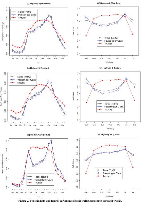
A thorough analysis was carried out to understand the hourly, daily traffic patterns of the classified vehicles (trucks and passenger cars). Figure 2 shows the typical daily and hourly variations of total traffic, passenger cars and trucks at the three study sites during winter months. The typical weekday hourly volume to AADT ratios (hourly factors) are shown in Figures 2(a), (c) and (d). The typical daily traffic volume to AADT ratios (daily factors) versus day of week plots are shown in Figures 2(b), (d) and (f). Because major portion of total traffic is passenger cars (80% to 85%), the traffic patterns of total traffic and passenger cars are very similar. However truck patterns are unique and different to passenger car patterns. The hourly passenger car factor variations show a single peak from 5 PM to 7 PM for the highway 2 sites (Figure 2(a) and Figure 2(c)). For the highway 2A site two distinct peaks are observed each day (Figure 2(e)): the morning peak from 7 AM to 9 AM and the evening peak from 4 PM to 7 PM. There is a general upward trend in weekday (Monday to Friday) passenger car traf-fic for all the study sites (see Figures 2(b), (d) and (f)). There is only a slight increase from Monday to Thursday; however, traffic on Friday traffic is substantially higher in all cases. The weekend passenger car traffic volumes are higher than the regular weekday (Monday to Thurs-day) passenger car traffic volumes and slightly less than Friday volumes for highway 2 sites (Figures 2(b) and (d)). For the highway 2A (Figure 2(f)), the Friday vol-umes are generally the highest, followed by Sunday, Sat-urday, and other weekdays. The differences in traffic patterns at the study sites show the need to conduct separate analysis. For trucks, the weekday hourly traffic patterns are different from passenger cars. Trucks show a

single peak from 2 PM to 6 PM. The daily truck volume patterns are also different as compared to passenger cars with weekday volumes significantly higher than week-ends and unlike passenger cars, Friday volumes are similar to other weekdays. Also truck traffic decreases significantly (more than 50%) during weekends as com-pared to weekdays. The traffic patterns in Figures 2(a) and (b) are very similar to the patterns in Figures 2(c) and (d). This indicates that the traffic conditions are very consistent on highway 2 with a similar traffic patterns for the two study sites located on highway 2. This is very helpful for testing the study findings for consistency. As per the road type classification system proposed by Sharma et al. [29] and traffic patterns observed in Figure 2, highway 2 sites can be classified as Regional Long Distance Roads and highway 2A site as a Commuter road. Because the traffic patterns for passenger cars and trucks are very distinct (as observed in Figure 2), modeling work has been carried out to develop separate models for the cars and trucks for Highway 2 and Highway 2A sites.

Literature indicates that a standard regression analysis is appropriate to quantify the association between high-way traffic volumes and weather. For example, Keay and Simmonds [8] successfully used regression analysis to quantify the impact of rainfall on road traffic volume. Furthermore, Knapp and Smithson [2] showed the ap-propriateness of the relationship between traffic volume and total snowfall using regression analysis. Based on these previous successful experiences, regression models are developed in this study to relate passenger car and truck traffic volumes with temperature and snowfall.

(6)

(a) Highway 2 (Red Deer)

Hour

H

o

u

rl

y

fa

c

to

r fo

r w

e

k

d

a

y

s

1hr 3hr 5hr 7hr 9hr 11hr 14hr 17hr 20hr 23hr

0.

0

.02

0.

04

0

.06

0

.08

0.

10

Total Traffic Passenger Cars Trucks

(b) Highway 2 (Red Deer)

Weekday

D

a

ily

f

a

c

to

rs

Sun Mon Tue Wed Thu Fri Sat

0

.0

0

.2

0

.4

0

.6

0

.8

1

.0

1

.2

1

.4

(c) Highway 2 (Leduc)

Hour

H

our

ly

f

a

ct

or

fo

r w

eek

days

0.

00

0.

02

0.

04

0.

06

0.

08

0.

10

(d) Highway 2 (Leduc)

Weekday

D

a

ily

f

a

c

to

rs

0

.0

0.

2

0.

4

0.

6

0.

8

1.

0

1.

2

1.

4

(e) Highway 2A (Leduc)

Hour

H

o

u

rl

y

fa

c

to

r fo

r w

e

k

d

a

y

s

0

.00

0

.02

0.

0

4

0.

0

6

0

.08

0.

1

0

(f) Highway 2A (Leduc)

Weekday

D

a

ily

f

a

c

to

rs

0.

0

0.

2

0.

4

0

.6

0

.8

1.

0

1.

2

1.

4

[image:6.595.71.527.80.734.2]

(7)

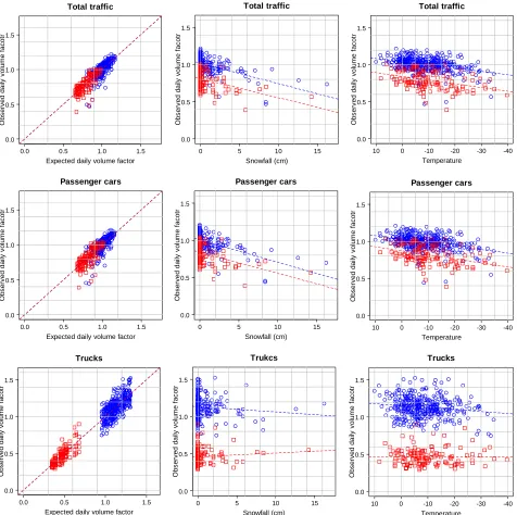
Figures 3 and 4 show the scatter plots between car and truck traffic volume factors versus expected volume factors, snowfall and temperature. An estimated regression line is also added in the same plot to show the level of closeness between the two values. The blue circles in these plots represent weekdays and red squares represent weekends. The scatter plots between daily volume fac-tors and expected daily volume facfac-tors show a very good cluster of sample data along the fitted regression line. This shows a strong positive linear relationship between daily volumes and historical average daily volumes (i.e.

expected daily volume factor). The blue circles and red squares overlap considerably in case of total traffic and car traffic plots. For trucks, the red squares are always on the lower side as compared to blue circles. This is be-cause of significantly lower truck traffic volumes on the weekends. It is worth noting that the weekday truck traf-fic factors are generally clustered between the values of 0.90 to 1.30. However, the weekend daily truck factors were found to spread between 0.30 and 0.70.

The regression lines of total vehicles and car volumes versus snowfall show moderate negative linear relationship,

0.0 0.5 1.0 1.5 0.0

0.5 1.0 1.5

Total traffic

Expected daily volume factor

O

b

se

rv

e

d

a

ily vo

lu

me

f

a

co

tr

0 5 10 15

0.0 0.5 1.0 1.5

Total traffic

Snowfall (cm)

O

b

se

rve

d

a

ily vo

lu

m

e

f

a

co

tr

10 0 -10 -20 -30 -40 0.0

0.5 1.0 1.5

Total traffic

Temperature

O

b

se

rv

e

d

a

ily vo

lu

me

f

a

co

tr

0.0 0.5 1.0 1.5 0.0

0.5 1.0 1.5

Passenger cars

Obs

erv

ed dai

ly

v

olum

e f

ac

ot

r

0 5 10 15

0.0 0.5 1.0 1.5

Passenger cars

Snowfall (cm)

O

b

se

rv

e

d

a

ily vo

lu

m

e

fa

c

o

tr

10 0 -10 -20 -30 -40 0.0

0.5 1.0 1.5

Passenger cars

Temperature

O

b

s

e

rve

d

a

ily

vo

lu

me

f

a

co

tr

0.0 0.5 1.0 1.5 0.0

0.5 1.0 1.5

Trucks

O

b

s

e

rve

d

a

ily vo

lu

m

e

fa

co

tr

0 5 10 15

0.0 0.5 1.0 1.5

Trukcs

Snowfall (cm)

Obs

er

v

ed daily

v

o

lum

e f

ac

ot

r

10 0 -10 -20 -30 -40 0.0

0.5 1.0 1.5

Trucks

Temperature

O

b

se

rv

e

d

a

ily v

o

lu

m

e

fa

co

[image:7.595.62.536.230.705.2]

tr

(8)

0.0 0.5 1.0 1.5 0.0

0.5 1.0 1.5

Total traffic

O

b

s

e

rv

e

d

a

ily

vo

lu

m

e

f

a

co

tr

0 5 10 15

0.0 0.5 1.0 1.5

Total traffic

Snowfall (cm)

O

b

se

rve

d

a

ily

vo

lu

me

f

a

co

tr

10 0 -10 -20 -30 -40 0.0

0.5 1.0 1.5

Total traffic

Temperature

Obs

e

rv

ed

dai

ly

v

o

lu

m

e

f

a

c

o

tr

0.0 0.5 1.0 1.5 0.0

0.5 1.0 1.5

Passenger cars

O

b

se

rv

e

d

a

ily

vo

lu

m

e

fa

co

tr

0 5 10 15

0.0 0.5 1.0 1.5

Passenger cars

Snowfall (cm)

O

b

se

rv

e

d

a

ily

vo

lu

m

e

fa

co

tr

10 0 -10 -20 -30 -40 0.0

0.5 1.0 1.5

Passenger cars

Temperature

Obs

erv

ed dai

ly

v

o

lu

m

e

f

ac

ot

r

0.0 0.5 1.0 1.5 0.0

0.5 1.0 1.5

Trucks

Obs

e

rv

ed dai

ly

v

o

lum

e

f

a

c

o

tr

0 5 10 15

0.0 0.5 1.0 1.5

Trukcs

Snowfall (cm)

O

b

se

rv

e

d

a

ily

vo

lu

m

e

fa

co

tr

10 0 -10 -20 -30 -40 0.0

0.5 1.0 1.5

Trucks

Temperature

Ob

s

erv

ed

dail

y

v

o

lum

e f

a

c

ot

[image:8.595.61.537.84.558.2]

r

Figure 4. Scatter plots between car and truck traffic volume factors versus snowfall and temperature in highway 2A WIM site (weekday traffic indicated by blue circle, weekend traffic by red square).

i.e., traffic volumes decrease with increase in amount of snowfall. A positive linear relationship is observed be-tween daily volumes and temperature, i.e., daily passen-ger car volumes increase with increase in daily average temperature. The slope of regression lines of both snow-fall and temperature plots are very similar between weekdays and Weekends. In the case of trucks, the clus-ters of observed data and the fitted regression lines fol-low similar very different as compared to cars. In case of trucks, the regression lines are very different for week-days and weekends. Similar patterns are observed for the

Highway 2A site in Figure 4. These observations support the need for the development of separate models for cars and trucks. The differences in weekday and weekend scat-ter plots, especially for trucks, stresses development of separate models for weekdays and weekends.

(9)

period). A correlation analysis was also conducted be-tween snowfall and temperature. The correlation coeffi-cients ranged from 0.03 to –0.18, which means that little to no correlation exists between snowfall and tempera-ture. This observation justifies the inclusion of snow and cold as independent variables in model specification.

5. Regression Model

5.1. Without Interaction of Snow and Temperature

Regression analysis has long been recognized as a most flexible and widely used technique to explain variation of quantitative dependent variable by establishing the rela-tionships between dependent variable and a specified set of independent variables in a form of additive and linear mathematical functions [30]. In this research, an attempt has been made to model the impact of weather factors on daily traffic volumes. For the purpose of initial mapping the relationships between daily traffic volume and weather factors, a regression model has been designed with three independent variables i.e., EDVF (expected daily volume factor), snow, and temperature. The addi-tive regression model formulated for this research is:





1 2 2

expected daliy volume factor,

snow fall, temperature

EDVF SNOW TEMP

i

i i

y f

  



   _i

(1)

where,

i: refers to the ith observation

1, 2, 3

   : regression coefficients estimated for the respective independent variable

i

y : estimated value of daily traffic volumes factor for different vehicle classes (cars, trucks etc.)

EDVF: expected daily volume factor

SNOW: amount of snowfall per day (cm)

TEMP: average daily temperature (˚C).

Normalized daily total volumes (traffic volume to AADT ratio), passenger car volumes (passenger car vol-ume to passenger car AADT ratio), and truck traffic volume (truck volume to truck AADT ratio) are used instead of actual volumes to take into consideration the yearly variations in traffic volumes. The normal traffic volume and weekly traffic trends are reflected by adding an ex-pected daily volume factor (EDVF) as an independent variable in model. EDVF is calculated using historical data of the same month, week, and day. The variables SNOW and TEMP represent the weather conditions.

5.2. With Interaction of Snow and Temperature

The additive regression model (Equation (1)) with EDVF, SNOW, and TEMP as independent variables would take into account the individual impact of cold and snowfall

on highway traffic (i.e., the impact of temperature on traffic volumes after impact of snowfall is taken into ac-count and the impact of each centimeter of snowfall after the effect of temperature is taken into account). A more complex model design is required to investigate whether the impact of snowfall on traffic volumes is the same at all temperature ranges or varies with the severity of tem-perature. Such analyses would verify the existence or non-existence of cold and snow interaction impacts on traffic volumes Therefore the model structure shown in Equation (1) is modified to accommodate interactions between cold (temperature) and snow. The differential impacts of snowfall by cold or, equivalently, the differ-ential impacts of cold by snowfall were captured in the model by including i interaction terms

to the earlier model design in Equation (1). The final form of the model used in this paper is shown in Equa-tion (2).

SNOW_iTEMP





1 2 3

4

expected daliy volume factor,

snow fall, temperature

EDVF SNOW TEMP

SNOW TEMP i

i i

y f

  



 



 



i

(2)

where,

4

 : regression coefficients estimated for the snow- temperature interaction variable.

Except interaction terms, all other terms serve the same purposes as defined in Equation (1).

6. Results and Analysis

The modeling process was carried out using the classi-fied WIM data and corresponding weather records from the three study WIM sites (two WIMs site for highway 2 and one WIM site for highway 2A). Regression models were calibrated using Equation (2). In total, 18 models (2 study highway sites × 3 day groups × 3 vehicle classes) were developed. These include separate models for all days, weekdays and weekends and for total traffic, pas-senger cars and trucks for both highways. Table 1 shows the 18 calibrated models along with the statistical test results.

The overall goodness of fit of the regression model to sample data is evaluated by the squared multiple correla-tion coefficient

 

R2 . The values for all models are over 0.98. The value of the

2

R

(10)

and are also calculated to test the null hypothesis of no interaction between snow and cold and the test re-sults are shown in Table 1.

2 Naive R

Based on the results of the four statistical tests (i.e., , F-test, incremental F-test, and t-test) conducted to evaluate the study models, it is apparent that the models fit well to the sample data and the structure of the pro-posed model is appropriate.

2

R

A partial effect analysis between the dependent vari-able and an independent varivari-able could be determined by varying the selected independent variable between its lower and upper boundaries (based on the study samples) and holding the other independent variables at a certain

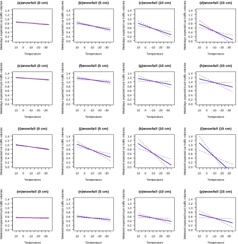
value. The partial effects of cold temperatures on daily traffic volumes are investigated in this section i.e., for example, partial effect of cold temperatures on daily traf-fic for a specitraf-fic pre-defined snowfall amount. Figures 5 and 6show the graphs developed to study the partial im-pact of cold temperatures on car and truck volumes. Re-sults are presented separately for weekdays and week-ends.

[image:10.595.59.538.267.729.2]

The solid line gives estimated daily traffic from the models shown in Table 1. The dotted lines give the 95% envelop for the upper and lower thresholds of dependent variable estimates. Each plot in Figures 5 and 6 shows the partial impact of cold temperatures on daily traffic

Table 1. Calibrated traffic weather models by vehicle class, day of the week and highway.

All Days Models (Highway 2A) Weekdays Models (Highway 2A) Weekend Models (Highway 2A)

Variables Total

Traffic

Passenger

Cars Trucks

Total Traffic

Passenger

Cars Trucks

Total Traffic

Passenger

Cars Trucks

EDVF 1.0329102*** 1.0374549*** 1.0010000*** 1.0266381*** 1.0309509*** 1.0028914*** 1.0605530*** 1.0637035*** 0.9907***

SNOW –0.0170572*** –0.0182616*** –0.0108900* –0.0155569*** –0.0169710*** –0.0085150 –0.0222481*** –0.0226961*** –0.11626**

TEMP 0.0020028*** 0.0022982*** 0.0000494 0.0015939*** 0.0018881*** 0.0001073 0.0032571*** 0.0035110*** –0.00001412

SNOWTEMP 0.0004917*_0.0006044*_–0.0009029* _0.0006064*_0.0006976** _–0.0003994 _{0.0001235 0.0003061}_–0.001941***

R2 0.9971 0.9968 0.9916 0.9977 0.9974 0.9923 0.9952 0.9948 0.9823

Statistic 43840***₃₉₂₂₀***₁₄₂₈₀***₃₉₅₀₀***₃₅₂₀₀***₁₁₂₉₀***₆₇₅₀***₆₂₈₇***₁₈₁₄***

Change

from 2

Naive

R - 0.0001 0.0001 0.0001 0.0001 - - - 0.0017

Incremental

F-Statistic - 15.8125

***_5.7857*_16.1304***_14.2692***_- _- _{- 28.9220}***

Number of

Sample Days 510 510 490 375 375 355 135 135 135

All Days Models (Highway 2) Weekdays Models (Highway 2) Weekend Models (Highway 2)

Variables Total Traffic Passenger

Cars Trucks

Total Traffic

Passenger

Cars Trucks

Total Traffic

Passenger

Cars Trucks

EDVF 1.0419390***_1.0463226***_1.0160252*** _1.0373627*** _1.0405659*** _1.0211869*** _1.0558368***_1.0606082***_1.0085723***

SNOW –0.0125431*** –0.0135735*** –0.0052943* –0.0144013*** –0.0153455*** –0.0080829** –0.0078173 –0.0102099 0.0051253

TEMP 0.0028608***_0.0030388***_0.0015290*** _0.0026138*** _0.0026134*** _0.0022545*** _0.0035069***_0.0040640***_0.0004533

SNOWTEMP 0.0009854*** 0.0011379*** 0.0002958 0.0007948** 0.0008879*** 0.0003974 0.0014021*** 0.0015639*** 0.0004921*

R2_0.9949_0.9936_0.9962_0.9953_0.994_0.9964_0.994_0.993_0.9957

Statistic 49690*** 39670*** 66770*** 39520*** 31070*** 52080*** 11030*** 9497*** 15520***

Change

from 2

Naive

R 0.0001 0.0001 - 0.0001 0.0001 - 0.0003 0.0003 0.0001

Incremental

F-Statistic 19.92

***

15.875*** - 15.8723*** 12.4333*** - 13.3*** 11.4*** 6.186*

Number of

Sample Days 1020 1020 1020 750 750 750 270 270 270

**

(11)

volumes for a specific combination of vehicle type, day of the week, location and pre-defined amount of snowfall. First row of plots in Figure 5 show the change in daily volume factor of passenger cars due to winter tempera-tures during weekdays for the Highway 2 sites for dif-ferent pre-defined amounts of snowfall. These plots are generated by fixing EDVF at its average value calculated from sample data set. It should be noted that the esti-mated daily volume factor at the point where the two dotted lines cross each other shows the average EDVF for that particular subset of data. Also note that the

crossing point generally happened at about –10˚C tem-perature which represents average and also most fre-quently occurring winter weather conditions in the vicin-ity of study sites. Comparison of slopes of plotted lines from left to right show change in partial impact of tem-perature on daily traffic with increase in amount of snowfall. Second row of plots in Figure 5 shows similar plots for trucks. Third and fourth rows of plots show the partial impact of cold on daily volume factor of passen-ger cars and trucks during weekends. The plots in Figure 6 are similar to Figure 5 except for different road site

(a)snowfall (0 cm)

Temperature W eek day s ex pec ted c ar t raf fic v olum es

10 0 -10 -20 -30 0.0 0.2 0.4 0.6 0.8 1.0 1.2 1.4

(b)snowfall (5 cm)

10 0 -10 -20 -30 0.0 0.2 0.4 0.6 0.8 1.0 1.2 1.4

(c)snowfall (10 cm)

10 0 -10 -20 -30 0.0 0.2 0.4 0.6 0.8 1.0 1.2 1.4

(d)snowfall (15 cm)

10 0 -10 -20 -30 0.0 0.2 0.4 0.6 0.8 1.0 1.2 1.4

(e)snowfall (0 cm)

Temperature W eek day s ex pec ted t ruc k t raf fic v olum es

10 0 -10 -20 -30 0.0 0.2 0.4 0.6 0.8 1.0 1.2 1.4

(f)snowfall (5 cm)

10 0 -10 -20 -30 0.0 0.2 0.4 0.6 0.8 1.0 1.2 1.4

(g)snowfall (10 cm)

10 0 -10 -20 -30 0.0 0.2 0.4 0.6 0.8 1.0 1.2 1.4

(h)snowfall (15 cm)

10 0 -10 -20 -30 0.0 0.2 0.4 0.6 0.8 1.0 1.2 1.4

(i)snowfall (0 cm)

Temperature W eek end ex pec ted c ar t raf fic v olum es

10 0 -10 -20 -30 0.0 0.2 0.4 0.6 0.8 1.0 1.2 1.4

(j)snowfall (5 cm)

10 0 -10 -20 -30 0.0 0.2 0.4 0.6 0.8 1.0 1.2 1.4

(k)snowfall (10 cm)

10 0 -10 -20 -30 0.0 0.2 0.4 0.6 0.8 1.0 1.2 1.4

(l)snowfall (15 cm)

10 0 -10 -20 -30 0.0 0.2 0.4 0.6 0.8 1.0 1.2 1.4

(m)snowfall (0 cm)

Temperature W eek end ex pec ted t ruc k t raf fic v olum es

10 0 -10 -20 -30 0.0 0.2 0.4 0.6 0.8 1.0 1.2 1.4

(n)snowfall (5 cm)

10 0 -10 -20 -30 0.0 0.2 0.4 0.6 0.8 1.0 1.2 1.4

(o)snowfall (10 cm)

10 0 -10 -20 -30 0.0 0.2 0.4 0.6 0.8 1.0 1.2 1.4

(p)snowfall (15 cm)

[image:11.595.67.533.230.708.2]

10 0 -10 -20 -30 0.0 0.2 0.4 0.6 0.8 1.0 1.2 1.4

(12)

(a)snowfall (0 cm) Temperature W e e kd a y s e xp e ct e d ca r t ra ff ic vo lu m e s

10 0 -10 -20 -30 0.0 0.2 0.4 0.6 0.8 1.0 1.2 1.4

(b)snowfall (5 cm)

Temperature W e e kd a y s e xp e ct e d ca r t ra ff ic vo lu m e s

10 0 -10 -20 -30 0.0 0.2 0.4 0.6 0.8 1.0 1.2 1.4

(c)snowfall (10 cm)

10 0 -10 -20 -30 0.0 0.2 0.4 0.6 0.8 1.0 1.2 1.4

(d)snowfall (15 cm)

10 0 -10 -20 -30 0.0 0.2 0.4 0.6 0.8 1.0 1.2 1.4

(e)snowfall (0 cm)

Temperature W e e kd a y s e xp e ct e d t ru c k t ra ff ic vo lu m e s

10 0 -10 -20 -30 0.0 0.2 0.4 0.6 0.8 1.0 1.2 1.4

(f)snowfall (5 cm)

10 0 -10 -20 -30 0.0 0.2 0.4 0.6 0.8 1.0 1.2 1.4

(g)snowfall (10 cm)

10 0 -10 -20 -30 0.0 0.2 0.4 0.6 0.8 1.0 1.2 1.4

(h)snowfall (15 cm)

10 0 -10 -20 -30 0.0 0.2 0.4 0.6 0.8 1.0 1.2 1.4

(i)snowfall (0 cm)

Temperature W eek e nd ex p ec ted c ar t ra ff ic v o lum es

10 0 -10 -20 -30 0.0 0.2 0.4 0.6 0.8 1.0 1.2 1.4

(j)snowfall (5 cm)

10 0 -10 -20 -30 0.0 0.2 0.4 0.6 0.8 1.0 1.2 1.4

(k)snowfall (10 cm)

10 0 -10 -20 -30 0.0 0.2 0.4 0.6 0.8 1.0 1.2 1.4

(l)snowfall (15 cm)

10 0 -10 -20 -30 0.0 0.2 0.4 0.6 0.8 1.0 1.2 1.4

(m)snowfall (0 cm)

Temperature W eek e nd ex p ec ted t ru c k t raf fic v ol um es

10 0 -10 -20 -30 0.0 0.2 0.4 0.6 0.8 1.0 1.2 1.4

(n)snowfall (5 cm)

10 0 -10 -20 -30 0.0 0.2 0.4 0.6 0.8 1.0 1.2 1.4

(o)snowfall (10 cm)

10 0 -10 -20 -30 0.0 0.2 0.4 0.6 0.8 1.0 1.2 1.4

(p)snowfall (15 cm)

[image:12.595.65.534.83.585.2]

10 0 -10 -20 -30 0.0 0.2 0.4 0.6 0.8 1.0 1.2 1.4

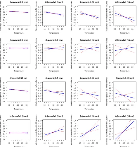
Figure 6. Partial impact of cold temperatures and snowfall on car and truck volumes for highway 2A Site (95% envelopes of volume estimates indicated by red dotted line, expected volume by blue solid line).

(Highway 2A site).

Based on the traffic weather patterns of Figure 5, the following interpretations can be made for Highway 2 sites, which serve regional long distance trips:

 There is a clear indication that traffic volume on a given day depends on severity of cold and amount of snowfall.

 A reduction in passenger car and truck volumes can be expected with increase in severity of cold

tem-peratures. The amount of decrease in traffic volume depends on severity of cold.

 When there is no snowfall the impact of cold tem-perature on both car and truck volumes is very mar-ginal (see plots in Figures 5(a), (e), (i) and (m)).  As the amount of snowfall increases the steepness of

(13)

This clearly shows the existence of cold and snowfall interactions.

 A snowfall of 15 cm or higher during severe cold conditions (–20˚C or lower) would result in a dra-matic decrease in passenger car traffic on the road (see plots in Figures 5(d) and (l)).

 With higher amounts of snowfall, passenger cars ex-perience higher reductions due to cold and snowfall as compared to trucks (as shown in plots d and l for cars; and plots h and p for trucks)

 For passenger cars, the weekend plots (Figures 5(i), (j), (k) and (l)) are steeper than weekdays (a, b, c, and d) indicating higher car traffic reductions in weekends as compared to weekdays. In the case of trucks, the regression lines seem parallel, which means the im-pact of cold and snow on truck traffic is similar for weekdays and weekends.

 It should be noted that the width of the 95% envelop (shown by dashed lines) also increases from left to right indicting that the reliability of model estimate deplete with increase in severity of weather condi-tions. This could be because of low sample size due to lesser number of days of heavy snowfall during the winter season.

The amount of reduction in traffic volume may be at-tributed to the proportion of discretionary trips in the traffic stream. The existence of more discretionary trips results in higher trip adjustments and, hence, higher traf-fic reductions. The reason of higher weekend traftraf-fic re-ductions may be due to the large proportion of discre-tionary trips during weekends. Trucks (or commercial vehicles) are usually required to follow rigid schedules to complete their mandatory travel irrespective of severe weather conditions. These kinds of business-oriented mandatory movements are most likely to generate unique truck travel patterns even when weather is unfavorable for making a trip. This could be the reason for (i) lower truck reductions in general and (ii) similar impact of weather on weekdays and weekends truck traffic

Figure 6 shows the partial impact of cold on car and truck traffic on Highway 2A site, which serves as a re-gional commuter road in Leduc region. Interpretation of plots is the same as in Figure 5. Similar to Highway 2, passenger car traffic experiences reduction in volume with increase in severity of cold and amount of snowfall. However, for both weekdays and weekends, the regres-sion lines seem to be less steep than those observed for Highway 2. This indicates lesser impact of cold on car traffic at Highway 2A site as compared to Highway 2. It is interesting to note that the width of the 95% envelops of volume estimates for Highway 2A site are larger as compared to the plots in Figure 5, especially for week-end car traffic. This could be due to a much smaller sam-ple size available for used in the analysis for Highway

2A site, as shown in Table 1. Except for these differ-ences, all the remaining observations made earlier based on passenger car traffic-weather relation plots in Figure 5 are valid for Highway 2A site also.

The behavior of truck traffic at Highway 2A site dur-ing adverse weather conditions is quite different from the Highway 2 site. It is very interesting to see the regression lines of truck traffic showing a reverse trend i.e., increase in truck traffic volume with increase in severity of weather conditions. Such an increase in truck traffic is marginal for weekdays and high for weekends. This is contradictory to what has been observed for truck traffic at Highway 2 site. Moreover, none of the studies in the literature reported increase in traffic volumes during se-vere weather conditions. A further investigation was conducted to understand the possible reasons for such a controversial truck traffic patterns.

After reviewing the highway network near the study site, it was found that Highway 814 runs parallel to the Highway 2A. Highway 814 is a secondary highway with lower priority for winter road maintenance (snow re-moval etc.). Therefore it is possible that truck drivers may change their travel route by shifting to Highway 2A. A careful analysis of hourly traffic data from permanent traffic counter site located on Highway 814 showed sig-nificantly lower traffic volumes during the days with severe weather conditions (i.e., higher than normal traffic reductions that were seen at other similar highway seg-ments). Brief communications with local municipalities in the vicinity of the study sites also indicated the possi-bility of traffic shifting. Therefore it could be concluded that there is a possibility of traffic volume increases on high standard highways during adverse weather condi-tions, which could happen due to shift of traffic from parallel low standard highways.

7. Summary and Conclusions

The literature study presented in this paper indicates clearly that severe weather conditions trigger variations in highway traffic. However, none of the past studies in the literature provided detailed information regarding impacts of winter weather on temporal and spatial varia-tions of truck traffic. It is believed that understanding of truck traffic variations (or behaviour) under severe weather conditions can benefit highway agencies in de-veloping such programs and policies as efficient moni-toring of passenger car and truck traffic, and plan for efficient winter roadway maintenance programs.

(14)

weather stations (operated by Environment Canada) in the province of Alberta. Multiple regression models were formulated and calibrated to relate truck and passenger car traffic variations to winter weather conditions. All the calibrated models were tested for statistical significance of the independent variables using the standard test sta-tistics such as F-test, incremental F-test, and t-test.

A number of conclusions were drawn from the study results. Firstly, both car and truck traffic volumes on highways vary with severity of cold and amount of snowfall. The impact of cold temperature on both car and truck volumes is marginal during no snowfall days. The reduction in traffic volume due to cold temperature would intensify with a rise in amount of snowfall indi-cating the existence of cold and snowfall interactions. With higher amounts of snowfall, passenger cars experi-ence higher reductions due to cold and snowfall as com-pared to trucks. A snowfall of 15 cm or higher during severe cold conditions (–20˚C or lower) would result in very few Cars travelling on the road. Moreover passenger cars experience higher traffic reductions in weekends as compared to weekdays. In the case of trucks the impact of cold and snow on truck traffic is similar for weekdays and weekends.

It is evident from this study that passenger cars are more vulnerable to adverse weather conditions than trucks. This vulnerability to severe weather conditions could be attributed to such behavior of drivers as choos-ing flexible departure times, changchoos-ing routes, or cancel-ing travel entirely and becancel-ing able to make trip adjust-ments by avoiding discretionary trips. Trucks are not as greatly affected as passenger cars by adverse weather conditions. Trucks (or commercial vehicles) are usually required to follow rigid schedules to complete their mandatory travel irrespective of severe weather condi-tions. These kinds of business-oriented mandatory movements are most likely to generate unique truck travel patterns even when weather is unfavorable for making a trip.

Interestingly, the modelling results for one of the study sites reveal that higher truck traffic volumes can result during heavy snowfall (or other adverse weather condi-tions) in winter months. This is contradictory to observa-tions from other similar studies in the literature. None of the studies in literature have reported such an increase in traffic volumes during severe weather conditions. A fur-ther investigation carried out for this study to understand the reasons for such behavior indicated shifting of trucks from secondary highways to primary highways due to poor winter maintenance programs. Therefore it can be concluded that there is a possibility of traffic volume increases on high standard highways during adverse weather conditions; which could happen due to shift of traffic from parallel low standard highways.

8. Acknowledgements

The authors are grateful towards the Natural Science and Engineering Research Council of Canada (NSERC), the Faculty of Graduate Studies at the University of Regina, and Saskatchewan Government Insurance (SGI) for their financial support. The authors also thank Alberta Infra-structure and Transportation for providing the WIM data used in this study.

REFERENCES

[1] S. Datla and S. Sharma, “Variation of Impact of Cold Temperature and Snowfall and Their Interaction on Traf-fic Volume,” In: Transportation Research Record: Jour-nal of the Transportation Research Board, No. 2169, Transportation Research Board of the National Acad-emies, Washington DC, 2010, pp. 107-115.

[2] K. K. Knapp and L. D. Smithson, “Winter Storm Event Volume Impact Analysis Using Multiple-Source Archived Monitoring Data,” In: Transportation Research Record: Journal of the Transportation Research Board, No. 1700, Transportation Research Board of the National Acad-emies, Washington DC, 2000, pp. 10-16.

[3] R. M. Hanbali and D. A. Kuemmel, “Traffic Volume Reduction Due to Winter Storm Conditions,” In: Trans-portation Research Record: Journal of the Transportation Research Board, No. 1387, Transportation Research Board of the National Academies, Washington DC, 1993, pp. 159-164.

[4] L. C. Goodwin, “Weather Impacts on Aterial Traffic Flow,” The Road Weather Management Program, FHWA, US Department of Transportation, Washington DC, 2002. [5] F. L. Hall and D. Barrow, “Effects of Weather and the

Relationship between Flow and Occupancy on Freeways,” In: Transportation Research Record: Journal of the Transportation Research Board, No. 1194, Transportation Research Board of the National Academies, Washington DC, 1988, pp. 55-63.

[6] Y. A. Hassan and J. J. Barker, “The Impact of Unseason-able or Extreme Weather on Traffic Activity within Lo-thian Region, Scotland,” Journal of Transport Geography, Vol. 7, No. 3, 1999, pp. 209-213.

doi:10.1016/S0966-6923(98)00047-7

[7] A. T. Ibrahim and F. L. Hall, “Effect of Adverse Weather Conditions on Speed-Flow-Occupancy Relationships,” In: Transportation Research Record: Journal of the Trans-portation Research Board, No. 1457, Transportation Re-search Board of the National Academies, Washington DC, 1994, pp. 184-191.

[8] K. Keay and I. Simmonds, “The Association of Rainfall and Other Weather Variables with Road Traffic Volume in Melbourne, Australia,” Accident Analysis and Preven-tion, Vol. 37, No. 1, 2005, pp. 109-124.

doi:10.1016/j.aap.2004.07.005

(15)

Board, No. 1948, Transportation Research Board of the National Academies, Washington DC, 2006, pp. 170-176. [10] B. L. Smith, K. G. Byrne, R. B. Copperman, S. M. Hennessy and N. J. Goodall, “An Investigation into the Impact of Rainfall on Freeway Traffic Flow,” Proceed-ings of the Annual Meeting of the Transportation Re-search Board, Washington DC, 2004.

[11] J. Andrey, B. Mills, M. Leahy and J. Suggett, “Weather as a Chronic Hazard for Road Transportation in Canadian Cities,” Natural Hazards, Vol. 28, No. 3, 2003, pp. 319- 343. doi:10.1023/A:1022934225431

[12] S. Datla and S. Sharma, “Impact of Cold and Snow on Temporal and Spatial Variations of Highway Traffic Volumes,” Journal of Transport Geography, Vol. 16, No. 5, 2008, pp. 358-372. doi:10.1016/j.jtrangeo.2007.12.003

[13] J. Fox, “An R Companion to Applied Regression,” SAGE Publications, Inc., Thousand Oaks, 2011.

[14] R Foundation for Statistical Computing, “R Development Core Team: A Language and Environment for Statistical Computing,” R Foundation for Statistical Computing, Vienna, 2010.

[15] S. A. Changnon, “Effects of Summer Precipitation on Urban Transportation,” Climatic Change, Vol. 32, No. 4, 1996, pp. 481-495. doi:10.1007/BF00140357

[16] J. C. McBride, M. C. Benlangie, W. J. Kennedy, F. R. McCornkie, R. M. Steward, C. C. Sy and J. H. Thuet, “Economic Impacts of Highway Snow and Ice Control,” FHWA, US Department of Transportation, Washington DC, 1997.

[17] V. P. Shah, A. D. Stern, L. C. Goodwin and P. Pisano, “Analysis of Weather Impacts on Traffic Flow in Metro-politan Washington DC,” Proceedings of the Annual Meeting of Institute of Transportation Engineers, Wash-ington DC, 2003.

[18] L. I. Zang, P. Holm and J. Colyar, “Identifying and As-sessing Key Weather-Related Parameters and Their Im-pact on Traffic Operations Using Simulation,” FHWA, US Department of Transportation, Washington DC, 2004. [19] J. Andrey and R. Olley, “Relationships between Weather and Road Safety, Past and Future Directions,” Clima-tological Bulletin, Vol. 24, No. 3, 1990, pp. 123-137. [20] P. J. Maki, “Adverse Weather Traffic Signal Timing,”

Proceedings of the Annual Meeting of Institute of Trans-portation Engineers, Las Vegas, 1999.

[21] A. J. Khattak, P. Kantor and F. M. Council, “Role of

Ad-verse Weather in Key Crash Types on Limited Access Roadway—Implications for Advanced Weather System,” In: Transportation Research Record: Journal of the Transportation Research Board, No. 1621, Transportation Research Board of the National Academies, Washington DC, 1998, pp. 10-19.

[22] ITT Industries, Inc., System Division, “Identifying and Assessing Key Weather-Related Parameters and Their Impacts on Traffic Operations Using Simulation,” FHWA, US Department of Transportation, Washington DC, 2003. [23] M. Kilpeläinen and H. Summala, “Effects of Weather and Weather Forecasts on Driver Behavior,” Transportation Research Part F: Traffic Psychology and Behaviour, Vol.10, No. 4, 2007, pp. 288-299.

doi:10.1016/j.trf.2006.11.002

[24] P. Kilburn, “Alberta Infrastructure & Transportation Weigh in Motion Report,” Government of Alberta Minis-try of Transportation, Calgary, 2008.

[25] Weather Office, Environment Canada, Gatineau, Quebec, Canada, 2010.

www.climate.weatheroffice.gc.ca/climateData/canada_e.h tml.

[26] “ArcGIS 10 Help Library: Geographic Information Sys-tem (GIS),” ArcGIS 10, Environmental SysSys-tem Research Institute, Inc., Redlands, 2010.

[27] J. H. Wyman, G. A. Braley and R. I. Stephens, “Field Evaluation of FHWA Vehicle Classification Categories,” FHWA, US Department of Transportation, Washington DC, 1985.

[28] Z. B., Liu and S. Sharma, “Statistical Investigations of Statutory Holiday Effects on Traffic Volumes,” In: Trans-portation Research Record: Journal of the Transportation Research Board, No. 1945, Transportation Research Board of the National Academies, Washington DC, 2006, pp. 40-48.

[29] S. Sharma and A. Werner, “Improved Method of Group-ing Province Wide Permanent Traffic Counters,” In: Transportation Research Record: Journal of the Trans-portation Research Board, No. 815, Transportation Re-search Board of the National Academies, Washington DC, 1981, pp. 12-18.