Enhanced Self Organizing Map Neural Network for DNA Sequence Classification

(1)

Enhanced Self-Organizing Map Neural Network for

DNA Sequence Classification

Marghny Mohamed1, Abeer A. Al-Mehdhar2, Mohamed Bamatraf2,Moheb R. Girgis3

1_{Faculty of Information and Computers, Assiut University, Assiut, Egypt}

2_{Faculty of Science, Hadhramout University of Science and Technology, Hadhramout, Yemen} 3_{Faculty of Science, Minia University, Minia, Egypt}

Email: [email protected], [email protected], [email protected], [email protected]

Received November 20, 2012; revised December 12, 2012; accepted December 19, 2012

ABSTRACT

The artificial neural networks (ANNs), among different soft computing methodologies are widely used to meet the challenges thrown by the main objectives of data mining classification techniques, due to their robust, powerful, dis- tributed, fault tolerant computing and capability to learn in a data-rich environment. ANNs has been used in several fields, showing high performance as classifiers. The problem of dealing with non numerical data is one major obstacle prevents using them with various data sets and several domains. Another problem is their complex structure and how hands to interprets. Self-Organizing Map (SOM) is type of neural systems that can be easily interpreted, but still can’t be used with non numerical data directly. This paper presents an enhanced SOM structure to cope with non numerical data. It used DNA sequences as the training dataset. Results show very good performance compared to other classifiers. For better evaluation both micro-array structure and their sequential representation as proteins were targeted as dataset accuracy is measured accordingly.

Keywords: Bioinformatics; Artificial Neural Networks; Self-Organizing Map; Classification; Sequence Alignment

1. Introduction

Bioinformatics could be defined as the science of man- aging and analyzing biological data using advanced computing techniques. One of the main challenges in this area is information discovery from the mass biological data [1]. Bioinformatics represents a new growing area of science to answer biological questions, and study of information presentation and transformation of biological systems using various computation techniques at several levels. Two important areas of bioinformatics: protein structure prediction (using both sequence matching and machine learning techniques); and data management. The major tasks of bioinformatics in the era of genome will be to find out what the genes really do in concerted action, either by simultaneous measurement of the activ-ity of arrays of DNA or by analyzing the cell’s protein complement. It will be hard to determine the function of many proteins experimentally, because the function may be related specifically to the native environment in which a particular organism lives. Many genes may be included in the genome for the purpose of securing survival in a particular environment, and may have no use in the artificial environment created in the laboratory [2].

Recently Self-Organizing Map (SOM) has received at-

tention as data mining knowledge discovery technique due to the highly beneficial properties [3-5]. A key characteristic of the SOM is its topology preserving ability to map a multi-dimensional input into a two-dimensional form. This qualifies SOM to be a good tool for data classification and clustering [6-8].

A data mining approach based on SOM as clustering, feature selection and classification, is introduced. SOM is employed by redesigning its several training phases to cope with the complex nature of DNA sequences, and integrating evolutionary techniques during learning process, using crossover and mutation to produce new features within the neighbor sequences of the wining unit in every iteration during training. Finally, set of class, cluster representative are generated. The main advantage of the proposed approach is that no interpretation phase is needed.

(2)

sequence and the alignment stops at the ends of regions of strong similarity, as an example for local technique is Smith-Waterman algorithm (SW).

Global alignment: identifies the similarity regions in the entire length from end to end in two or more sequences. There are many algorithms applied in the problem of sequence alignment like Dynamic Programming (DP), it is slow but optimal. The general global technique based on dynamic programming is Needleman-Wunsch algorithm (NM&W).

The rest of the paper is organized as follows: Section 2 presents a background of DNA sequences classification techniques. Section 3 describes the SOM algorithm. Sec- tion 4 describes the phases of the proposed system. Sec- tion 5 presents the experimental results, and Section 6 concludes the paper.

2. Background

During the past decades, advances in genomics have generated a wealth of biological data, increasing the dis- crepancy between what is observed and what is actually known about life’s organization at the molecular level. To gain a deeper understanding of the processes under- lying the observed data, pattern recognition techniques play an essential role.

The machine learning techniques were generally applied for the following problems: classification, clustering, construction of probabilistic graphical models, and optimization.

The goal of the classification is to divide objects into classes, based on the characteristics of the objects.

The rule that is used to assign an object to a particular class is termed the classification function, classification model, or classifier. The problems in bioinformatics can be cast into a classification problem, and well established methods can then be used to solve the task [9-11]. The classification of micro-array data is often the first step towards a more detailed analysis of the organism as in [12, 13].

DNA sequences classification is a main class of problems in bioinformatics that depends on the topic of clustering, also termed unsupervised learning, because no class information is known a priori. The clustering goals is to find natural groups of (clusters) in the data that is being constructed, where objects in one cluster should be similar to each other, while being at the same time different from the objects in another cluster. The clustering in bioinformatics is concerned with the clustering of mi- croarray expression data [14,15], and the grouping of sequences, e.g. to build phylogenetic tree. Formally, they represent multivariate joint probability densities via a product of terms, each of which only involves a few variables. The structure of the problem is then modeled

using a graph that represents the relations between the variables, which allows to reason about the properties entailed by the product. Examples are Bayesian methods for constructing phylogenetic trees [16]. The prediction of protein structure is the other example of applications of machine learning techniques in bioinformatics, in which the problem can be formalized into an optimization problem, that includes motif identification in sequences, and the combination of different sources of evi- dence for analysis of global properties of bio(chemical) networks. In all of these domains, machine learning techniques have proven their value, and new methods are constantly being developed [17].

Additionally, many problems in computational biology involve searching for unknown repeated patterns, often called motifs, and identifying regularities in nucleic or protein sequences. Both imply inferring patterns, of unknown content at first, from one or more sequences. Regularities in a sequence may come under many guises. They may correspond to approximate repetitions randomly dispersed along the sequence, or to repetitions that occur in a periodic or approximately periodic fashion. The length and number of repeated elements one wishes to be able to identify may be highly variable [18].

The algorithms of motif discovery can be split into two categories: exhaustive or heuristic methods. In the former, the algorithms evaluate the statistical significance of all possible motifs, and output a ranked list. This approach is efficient since it spares from the need of pre-selecting a subset of motifs to use in the classification. That has also the merit of achieving better performances than most of the other methods introduced for the same task [19]. Unlike this approach, we generate artificial sequence; this sequence automation includes the target motif. The generated sequence is a general representation of its motifs. This is achieved by enhancing classification algorithm that predicts whether sequence may contain to a given set of similarity sequence without extracting information from the sequence. The classifier needs a training set composed of a similarity of positive set, and a ne- gative set, comprising sequencing of the genes not re-lated to the first group. In other words, the classifier de-termines, from the randomly selected genes, whether it is likely to be co-expressed with the sequence of the posi-tive set or not. This is based on sequence alignment ran-domly selected genes.

(3)

Algorithm, which applies more sensitive approach to the alignment of strings with different lengths [22]. Simu- lated Annealing (SA) was one of the first heuristics applied to sequence alignment [23-25], over time, GA and many variants of it have been applied to the sequence alignment problem. Shyu et al. reviewed the strengths and disadvantage of their recent application for sequence alignment using evolutionary computation [26], which combined ant colony optimization (ACO) with GA to overcome the problem of becoming trapped in local optimum. ACO was applied on the best alignment of the GA approach to find a globally optimum solution ACO is also used to align sequences. Avoidance of the local optimum was achieved by adaptively adjusting the parame- ters and updating the pheromones.

3. Self-Organizing Map

Data mining is an area that, extract the hidden predictive information from large data with its powerful technology. One main objectives of data mining is classification learning. Classification assigns items in a collection to target categories or classes. The goal of classification is to ac- curately predict the target class for each case in the data.

Self-Organizing Map (SOM) is one of the widely applied neural networks and has some interesting features over other neural networks. One advantages of using SOM is that it is quite robust with respect to noisy data, and its advantages over other classification models are its natural robustness and its very good illustrative power. Indeed, it has been successfully applied for several classification tasks.

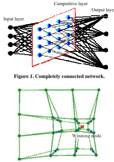
[image:3.595.320.518.436.717.2]

SOM does not require an external teacher during the training phase. Therefore, SOM classified as unsupervised neural networks. The SOM receives a number of input patterns, discovers significant features in these patterns and learns how to classify input data into appropriate categories. SOM has the best characteristic which projects high-dimensional data onto a low-dimensional grid and the topological order of the original data was visually reveals. It was developed in 1982 by Tuevo Ko- honen, a professor emeritus of the Academy of Finland [27]. SOM is a feed forward network and completely connected. Feed forward networks do not allow looping. Figure 1 shows SOM structure as completely connected.

SOM can also be viewed as a constrained version of k-means clustering [28], in which the cluster centers tend to lie in a low-dimensional manifold in the feature or attribute space. With SOM, clustering is performed by having several units competing for the current object. The unit whose weight vector is closest to the current object becomes the winning or best matching unite (BMU). So as to move even closer to the input object, the weights of the winning unit are adjusted, as well as those

of its nearest neighbors as shown in Figure 2.

The SOM Algorithm Can Be Expressed as Following

1) Initialization: choose random values for the initial weight vectors wj, and assign a small positive value to the

learning rate parameter .

2) Activation:apply the input vector X to activate the SOM network, and find Similarity Matching the BMU neuron Xi at iteration p, using the norm of minimum

Euclidean distance usual measure as in “Equation (1)”,

 

2

1

min

1, 2, ,

n

j i ij

j

i

E W p X W p

j m



 

   _  _







X

(1)

where n is the number of neurons in the input layer, and m is the number of neurons in the SOM layer.

3) Updating: Apply the weight update equation



1



 

     



 



ij ij

W p W p   P  P X p W p



(2)

where Θ is restraint due to distance from BMU usually called the neighborhood function,  t



is the learning rat, and W_ij

 

p

4) Continuation:return to step 2 until the feature map stops changing, or no noticeable changes occur in the feature map.

is the weight repairing in pth iteration.

After processing all of the input, the result should be a

Input layer

Competitive layer

Output layer

Figure 1. Completely connected network.

(4)

w m n



spatial organization of the input data organized into similar regions.

Set first row and column to 0’s and create a matrix with U + 1 Rows and T + 1 Columns.

4. The Proposed System

4.2.2. Scoring Scheme

The score matrix cells are filled row by row starting from the C (2, 2), where: match score = +1; mismatch score =

−1; g = gap penalty = −1; The phases of the proposed system are described in the

following subsections.

The first row and the first column of the score matrix are filled as multiple of gap penalty.

4.1. Phase I: Data Representation



Score of any cell C i j,







 









dig 1, 1 ,

max up 1,

left , 1

C i j S i j

C i j g

C i j g

 _ _ _{ }

 _ _ _



 _ _{ }



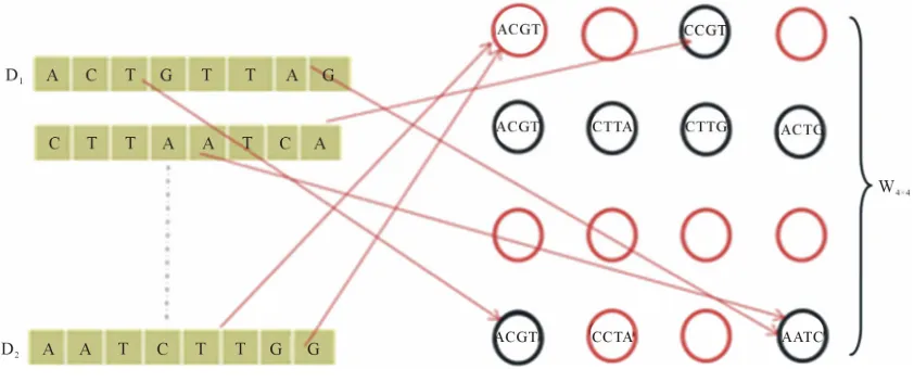
is the maximum of: Redesigning the SOM node structure to handle the DNA

sequence. Let

 

be the set of SOM nodes (weight), (where m is height and n is width). Every w 

[image:4.595.89.510.550.726.2]

, represents the vector set of length k as shown in Figure 3, where k is an integer between minimum length and maximum length of the input data

 

wij

(3)



D , representing the number of input sequences. In addition to set of elements in every sequence w contains additional blocks to store the class counter

 

z

C which will be used in the training phase, where Z is set of the number of classes present in the input data. The node structure is shown in Figure 4.

 

,

S i j is the substitution score for letters i and j. where

4.2. Phase II: Training

In this phase the same idea of SOM training is used as described in Section 3 except for the similarity function and the neighborhood update. Initially SOM weights are set to random examples from input data, ij, wij = Dy.

Traditional SOM can’t handle neither dynamic nor char- acter based data since Euclidean distance “Equation (1)” and “Equation (2)” are used to compute or measure dif- ferences between numeric values, instead we use Nee- dleman & Wunsch algorithm, to calculate the difference between the Dij and Wij as follows:

w 

 

,

C i j 4.2.1. Initialization of the Score Matrix

The cell of score matrix are labeled where i = 1, 2, ···, U, j = 1, 2, ···, T.

The value of the cell C i

 

depends only on the values of the immediately adjacent northwest diagonal, up and left cells, as shown in Figure 5.

,j

After filling score matrix the last cell has the maximum alignment score.

4.2.3. Trace Back

Traceback is the process of deduction of the best alignment from the score matrix.

Trace back starts from the last cell bottom-right corner in the score matrix. There are three possible moves: di- agonally (toward the top-left corner of the matrix), up, or left. The traceback is completed when the first, top-left cell of the matrix is reached.

After selecting the wining node wij, the neighbor nodes

are selected as “Equation (2)”.

As stated previously, SOM algorithm is designed for unsupervised learning. To use SOM for supervised learning (classification), enhanced node structure is used (as described in phase I). Additional blocks where employed. These blocks were initially set to zero at every step. If the node is selected as winner the class counter of the

(5)

corresponding class of the selected example is incremented by one shown as in Figure 6.

Every node wij in SOM network is connected to the

data , by connecting weight, set of winning class counters _m, ₁ ₂ m where m is the num-

ber of classes, as shown in Figure 6.

 

D

, , ,

c c  c

 

D

k



BMU



To understand that the technique provides the possibil- ity of utilizing the class label provided in the training set while training the SOM, we can simply say that the vector BMU is introduced to the node structure to provide a voting criterion, so that such nodes with maximum BMUi

are dragged during the weight update process. Shifting such nodes towards the wining node which is definitely of the same class increases the means of relationship between such nodes, at the same time leaving nodes from other classes decreasing the relationship between such nodes and their un-similar neighbors.

The main idea in our proposed method is to measure the similarity between objects independently from the data by using new distance NM&W, after determined wining node, then {BMU}I increased by one for ith_{of class}

counter. This confidence indicates a similarity between both the input data _k and the winning node BMU.

[image:5.595.321.517.322.566.2]

In the last step weight update is performed as shown in Figure 7. In conventional SOM all nodes act in blinded path in the state of the wining node, while in the proposed method we have overcome this problem as follows: before updating weight connection, the only set of nodes in the neighborhood with maximum class counter equal to the current instance class label will be considered as neighbor nodes.

In addition, the winning SOM unit is the unit Wij who

has the smallest distance to each instance, the appropriate class counter of the winning unit is incremented by one. After all instances have been presented, the largest class counter of each unit defines its label see phase III, and then calculates the reliability of all instances by “Reli- ability Equation” below.

Number of time the label Reliability

The total number of l 

Weight Update:

To increase the similarity between neighborhood nodes we introduce crossover and mutation. These operations will reproduce modified sequence oriented to the wining node and the current instance as well. For all nodes in the neighborhood of the BMU, crossover and mutation are performed as shown in Figures 8 and 9.

Number of crossover points is selected randomly and the value decreases based on how close gi from nij. The

node with high score with the wining node is selected and replaced with gi.

The mutation step is applied here to reduce the local- minima that might be caused by the crossover step and prevents the algorithm diversity towards the wining nodes and the data.

4.3. Phase III

The generated SOM is then categorized based on generated

was counted abels

1 2 1 2 1 2 1 2

1 2 z 1 2 z 1 2 z 1 2 z

n

C ,C , ,C C ,C , ,C C ,C , ,C C ,C , ,C

C ,C , ,C C ,C , ,C C ,C , ,C C ,C , ,C m

C ,C , ,C C ,C , ,C C ,C , ,C C ,C , ,C

z z z z

   

ACG. , TCG. , ACG. , CTG. ,

CCG. , ACG. , TTG. , TCG. ,

TCG. , CCG. , TTG. , ACG. ,

CCG. ,

   

 TCG. , CCG., TTG.,

1 2 z 1 2 z 1 2 z 1 2 z

C ,C , ,C C ,C , ,C C ,C , ,C C ,C , ,C

A C T T G ··· C1 C2 ··· CZ

Figure 4. Node structure.

 1,  C i j

 1, 1

C i j C i j, 1

 ,

C i j 

Figure 5. The value of the cell C (i, j).

[image:5.595.120.516.324.727.2]

(6)

Cluster 1

[image:6.595.61.283.80.409.2]

Cluste Cluster 2

Figure 7. Performing weight update.

Figure 8. Crossover.

Figure 9. Mutation.

reliability in “Reliability Equation”, as shown in Figure 10.

[image:6.595.309.535.85.562.2]

4.4. SOM Flowchart

Figure 11 shows the flowchart of the proposed SOM.

5. Experiment Result and Discussions

We have used dataset from the web site NCBI (The Na- tional Center for Biotechnology Information) advances science and health by providing access to biomedical and genomic information [29], and aging dataset (the datasets created in this work have, depending on the criteria used between 135 and 148 data instances, out of which 33 represent ageing-related DNA repair genes and the re- maining represent non-ageing-related DNA repair genes) [30]. Both set where represented as a protein sequence and micro array DNA.

E.G:

Sequential data set:

>gi|224515018|ref|NT_022517.18| Homo sapiens chromosome 3 TCCTCCCAGAATCTGGAGAGGTCAACCTGTTCTTCAAA CAAAACAGATACAGCACCAAACATGAAAAGCATTGAA ATCTGGAGAGGTCAACCTGTTCTTCAAAAGAATCTGGA

GAGGTCAACCTGCTTCAAACAAAACAG CAAAACAG

GATCCTGGGGTTGAAAGTCGGCAGAGGGCATTCTGAT

r 3

Figure 10. The output map.

Initialize Weight (wij) randomly Start

Compute the distance between Dj and Wij by using Needleman

and Wunsch

Select wij how scan is max

Update the weights of the winning neuron and its neighborhood X{gi} of nij using Multi point crossover & mutation

NO Stopping criterion Sequentially selectdata

Input Dj

Yes

End

Figure 11. Flowchart of the proposed SOM.

Later EuGene [31] home and MEME [32] are used for sample result analysis, verification and visualization.

The selected data set is applied to the proposed system after partitioning them into test and training. The same data sets were applied to other classifiers using weka and results are generated as shown inTable 1.

These accuracy and Precision are computed as follows:

TP TN

Accuracy 100%

TP TN FP FN 

 

   (3)

TP Precision

TP FP 

(7)

[image:7.595.55.540.84.311.2] [image:7.595.310.536.334.461.2]

Figure 12. Results generated by MEME and EuGene’Hom.

Table 1. Example of chromos

Chromosomes Name Length omes length.

Chromosome 1 245,522,847 bp

sifiers results u

Technique Name Precision Overall Accuracy

Table 2. Clas sing weka.

Naïve Bayes 0.841 79

Voted Perceptron 0.761 76

JRip 0.916 81

OneR 0.952 86

[image:7.595.62.286.352.439.2]

J48 0.953 87

Figure 13. Accuracy compared to the other classifiers.

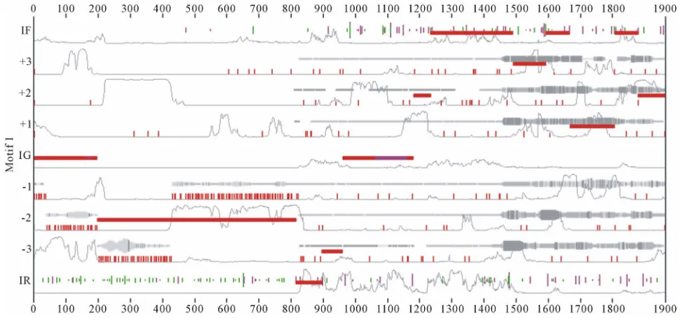
from the results generated by MEME and EuGene’Hom (see Figure 12), which are similar and general at some regions. Moreover this indicates that at the learning pro

cess ne ry

a

B

dealing with this data moti- vated us to introduce an enhanced SOM structure algo- ake it easier to deal with DNA se-

Ran ee

Enhanced SOM

dom Tr 0.886 77

0.952 86

T ystem co ely shows per-

rmance in terms of precision and accuracy. he proposed s mparativ a good fo

The generated representative sequences (chromosomes) could successfully cover test exemplars, in our system we applied different example of chromosomes length as shown in Table 2.

At the same time from the visualization of sample chromosome 3, we can manually notice the set of motifs generated automatically during the learning process.

Another proof for system efficiency could be noticed

- wly extracted sequences due to the evolutiona ture at phase II.

n

The performance of the proposed system is acceptable in terms of accuracy compared to the other classifiers as shown in Figure 13.

6. Conclusions

ioinformatics requires handling large volumes of mi- croarray data, involving natural interaction with information science. Difficulty in

rithm, in order to m

[image:7.595.59.286.467.602.2]

(8)

is measured accordingly.

In the proposed model custom crossover and random mutation guide the training process towards good newly generated representatives, eliminating the weak regions without getting trapped to local minima. The performance of Needleman and Wunsch algorithm performed very well in selecting the best match unit (BMU). The ex

[2] P. Baldi and S. Brun atics the Machine

Learning App sachusetts Institute

. McGarry, S. Wermter and C. Bowerman, perimental results indicated that the performance of the proposed system is acceptable in terms of accuracy compared to the other classifiers.

REFERENCES

[1] P. Khandheria and H. R. Garner, “Developing a Modern Web Interface for Database-Driven Bioinformatics Tools,” Engineering in Medicine and Biology Magazine, Vol. 26, No. 2, 2007, pp. 96-98.

ak, “Bioinform roach,” 2nd Edition, Mas of Technology, Cambridge, 2001.

[3] S. K. Shukla, S. Rungta and L. K. Sharma, “Self-Orga-nizing Map Based Clustering Approach for Trajectory Data,” International Journal of Computer Trends and Technology (IJCTT), Vol. 3, No. 3, 2012, pp. 321-324. [4] L. K. Sharma and S. Rungta, “Comparative Study of Data

Cluster Analysis for Microarra,” International Journal of Computer Trends and Technology (IJCTT), Vol. 3, No. 3, 2012, pp. 387-390.

[5] S. K. Bhatia and V. S. Dixit, “A Propound Method for the Improvement of Cluster Quality,” International Journal of Computer Science Issues (IJCSI), Vol. 9, No. 2, 2012, pp. 216-222.

[6] M. S. Babu, N. Geethanjali and B. Satyanarayana, “Clus-tering Approach to Stock Market Prediction,” Advanced Networking and Applications, Vol. 3, No. 4, 2012, pp. 1281-1291.

[7] R. Krakovsky and R. Forgac, “Neural Network Approach to Multidimensional Data Classification via Clustering,” IEEE 9th International Symposium on Intelligent Systems and Informatics (SISY), Subotica, 8-10 September 2011, pp. 169-174.

[8] J. Malone, K

“Data Mining Using Rule Extraction from Kohonen Self- Organizing Maps,” Neural Computing & Applications, Vol. 15, No. 1, 2005, pp. 9-17.

doi:10.1007/s00521-005-0002-1

[9] C. Burge and S. Karlin, “Prediction of Complete Gene Structures in Human Genomic DNA,” Journal of Mole- cular Biology, Vol. 268, No. 1, 1997, pp. 78-94. doi:10.1006/jmbi.1997.0951

[10] C. Mathé, M. F. Sagot, T. Schiex Methods of Gene Prediction, Their

and P. Rouzé, “Curr Strengths and

Weak-ent

nesses,” Nucleic Acids Research, Vol. 30, No. 19, 2002, pp. 4103-4117. doi:10.1093/nar/gkf543

[11] S. L. Salzberg, M. Pertea, A. L. Delcher, M. J. G and H. Tettelin, “Interpolate

a d Markov Models for karyotic Gene Finding,” Genomics, Vol. 59, No. 1, 1999,

rdner, Eu-

pp. 24-31. doi:10.1006/geno.1999.5854

[12] T. Golub, D. Slonim, P. Tamayo, C. Huard, M. Gaasen- beek, J. Mesirov, H. Coller, M. Loh, J. Downing and M. Caligiuri, “Molecular Classification of Cancer: Class Dis- covery and Class Prediction by Gene Expression Moni- toring,” Science, Vol. 286, No. 5439, 1999, pp. 531-537. doi:10.1126/science.286.5439.531

[13] I. Inza, P. Larranaga, R. Blanco and A. J. Cerrolaza,

“Fil-entifying Distinct Sets ter versus Wrapper Gene Selection Approaches in DNA Micro-Array Domains,” Artificial Intelligence in Medi- cine, Vol. 31, No. 2, 2004, pp. 91-103.

[14] T. Hastie, R. Tibshirani, M. B. Eisen, A. Alizadeh, R. Levy, L. Staudt, W. C. Chan, D. Botstein and P. Brown, “Gene Shaving as a Method for Id

of Genes with Similar Expression Patterns,” Genome Bi- ology, Vol. 1, No. 2, 2000, pp. 3.1-3.21.

doi:10.1186/gb-2000-1-2-research0003

[15] Q. Sheng, Y. Moreau and B. De Moor, “Biclustering Mi- cro-Array Data by Gibbs Sampling,” Bioinformatics, Vol. 19, No. S2, 2003, pp. 196-205.

doi:10.1093/bioinformatics/btg1078

[16] F. Ronquist and J. P. Huelsenbeck, “MRBAYES 3: Ba- yesian Phylogenetic Inference under M

Bioinformatics, Vol. 19, No. 12, 2003, p

ixed Models,” p. 1572-1574. doi:10.1093/bioinformatics/btg180

[17] P. Larranaga, B. Calvo, R. Santana, C. Bielza, J. Galdiano, I. Inza, J. A. Lozano, R. Armánanzas

Perez and V. Robles, “Machine Lear

, R. Santafe, A. ning in Bioinformat-ics,” Briefings in Bioinformatics, Vol. 7, No. 1, 2006, pp. 86-112. doi:10.1093/bib/bbk007

[18] C. Iliopoulos, K. Perdikuri, E. Theodoridis, A. Tsakali and K. Tsichlas, “Algorithms for E

dis xtracting Motifs from Biological Weighted Sequences,” Original Research Arti- cle Journal of Discrete Algorithms, Vol. 5, No. 2, 2007, pp. 229-242. doi:10.1016/j.jda.2006.03.018

[19] M. Tompa, N. Li, T. L. Bailey, G. M. Church, B. De Moor, E. Eskin, A. V. Favorov, M. C. Frith, Y. Fu, W. J.

ctor Binding Kent, V. J. Makeev, A. A. Mironov, W. S. Noble, G. Pa- vesi, G. Pesole, M. Regnier, N. Simonis, S. Sinha, G. Thijs, J. van Helden, M. Vandenbogaert, Z. Weng, C. Workman, C. Ye and Z. Zhu, “Assessing Computational Tools for the Discovery of Transcription Fa

Sites,” Nature Biotechnology, Vol. 23, No. 1, 2005, pp. 137-144. doi:10.1038/nbt1053

[20] S. B. Needleman and C. D. Wunsch, “A General Method Applicable to the Search for Similarities in the Amino Acid Sequence of Two Proteins,” Journal of Molecular Biology, Vol. 48, No. 3, 1970, pp. 443-453.

doi:10.1016/0022-2836(70)90057-4

[21] H. J. Böckenhauer and D. Bongartz, “Algorithmic Aspects of Bioinformatics,” Springer, Berlin, 2007.

ent by Par-

Multiple Se- [22] A. Polanski and M. Kimmel, “Bioinformatics,” Springer,

Berlin, 2007.

[23] M. Ishikawa, T. Toya, M. Hoshida, K. Nitta, A. Ogiwara and M. Kanehisa, “Multiple Sequence Alignm

allel Simulated Annealing,” Computer Applications in the Biosciences, Vol. 9, No. 3, 1993, pp. 267-273.

(9)

tions in the Biosciences, Vol. 10, No. 4,

ensus Se-quence Alignment Using Simulated Annealing,” Com- puter Applica

1994, pp. 419-426.

[25] J. M. Keith, P. Adams, D. Bryant, D. P. Kroese, K. R. Mitchelson, D. A. E. Cochran and G. H. Lala, “A Simu- lated Annealing Algorithm for Finding Cons

quences,” Bioinformatics, Vol. 18, No. 11, 2002, pp. 1494-1499. doi:10.1093/bioinformatics/18.11.1494 [26] C. Shyu, L. Sheneman and J. A. Foster, “Multiple Se-

quence Alignment with Evolutionary Computation,” Ge- netic Programming and Evolvable Machines, Vol. 5, No. 2, 2004, pp. 121-144.

doi:10.1023/B:GENP.0000023684.05565.78

[27] J. Vesanto and E. Alhoniemi, “Clustering of the Self-Or-

ganizing Map,” IEEE Transactions on Neural Networks, Vol. 11, No. 3, 2000, pp. 586-600.

doi:10.1109/72.846731

[28] J. W. Michael, “Using Data Clustering as a Method of Estimating the Risk of Establishment of Bacterial Crop Diseases,” Computational Ecology

No. 1, 2011, pp. 1-13. and Software, Vol. 1,

eme.cgi [29] http://www.ncbi.nlm.nih.gov/guide/

[30] http://tata.toulouse.inra.fr/apps/eugene/EuGeneHom/cgi-b in/EuGeneHom.pl