Multiple Action Sequence Learning and Automatic Generation for a Humanoid Robot Using RNNPB and Reinforcement Learning

(1)

Multiple Action Sequence Learning and Automatic

Generation for a Humanoid Robot Using RNNPB

and Reinforcement Learning

Takashi Kuremoto

1

, Koichi Hashiguchi

1

, Keita Morisaki

1

, Shun Watanabe

1

, Kunikazu Kobayashi

2

,

Shingo Mabu

1

, Masanao Obayashi

1

Graduate School of Science and Engineering, Yamaguchi University, Ube, Yamaguchi, Japan; 2School of Information Science and Technology, Aichi Prefectural University, Nagakute, Aichi, Japan.

Email: [email protected]

Received Month Day, Year (2012).

ABSTRACT

This paper proposes how to learn and generate multiple action sequences of a humanoid robot. At first, all the basic action sequences, also called primitive behaviors, are learned by a recurrent neural network with parametric bias (RNNPB) and the value of the internal nodes which are parametric bias (PB) determining the output with different pri-mitive behaviors are obtained. The training of the RNN uses back propagation through time (BPTT) method. After that, to generate the learned behaviors, or a more complex behavior which is the combination of the primitive behaviors, a reinforcement learning algorithm: Q-learning (QL) is adopt to determine which PB value is adaptive for the generation. Finally, using a real humanoid robot, the proposed method was confirmed its effectiveness by the results of experiment.

Keywords: RNNPB; Humanoid Robot; BPTT; Reinforcement Learning; Multiple Action Sequences

1.

Introduction

To recognize, learn, and generate adaptive behaviors for an intelligent social robot is a charming theme and it has been attracting researchers more than a decade. From the view that dynamic complex behaviors of the robot are composed by the spatiotemporal changed actions which are so-called “primitive behaviors”, or “element actions”, gesture recognition has been approached by lots of me-thods such as 3D models [1], self-organizing map (SOM) [2,3], hidden Markov model (HMM) [4-7], dynamic Baysian network (DBN) [8], recurrent neural network (RNN) [9-11], and dynamic programming (DP) [12].

Tani with his colleagues proposed a RNN with para-metric bias (RNNPB) which realize not only recognition of multiple behaviors but also learning and generation of them, based the finding of mirror neuron system in the brain [13,14]. The input of RNNPB includes sensory (visual or auditory) information and teacher’s motor in-formation during the learning period, and the imitative behaviors are output (generated) by the network accord-ing to the observation of robot in the period of genera-tion.

In this paper, we propose to combine RNNPB and reinforcement learning (RL) [15] to realize (i) the

mul-tiple behaviors automatic generation or (ii) by the in-struction of a human instructor. In another word, the adaptive PB values are determined as the result of RL in the generation process. Various patterns of primitive behaviors are learned by back-propagation through time (BPTT) [16] [17], and PB vectors are obtained as the result. Considering the PB vectors as finite states of a Markov decision process (MDP), a complex behavior can be learned as an optimal state transition process of these primitive behavior patterns using the RL algorithm such as Q-Learning. Using a humanoid robot “PALRO” (Fujisoft Inc., 2010), experiments results confirmed the effectiveness of the proposed method.

2.

Proposed System

(2)

input of the network, to meet the different patterns of primitive behaviors; (iii) Explore the temporal order of different parameter bias (PB) vectors, which yields different primitive behaviors, by the reinforcement learning (RL) algorithm [15]. The details of the proposed method are given in this section.

2.1.

RNNPB

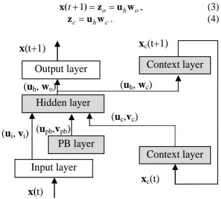
The recurrent neural network with parametric biases (RNNPB) [9-11] is a Jordan-type recurrent feed forward neural network [18] with three kinds of internal layers: hidden layer, context layer and parametric bias (PB) layer (Figure 1). Nodes in Hidden layer and Context layer have their internal states with sigmoid function:

z

z ₋_α

+ = e f 1 1 )

( . (1)

where α, a positive constant, is the gradient of the function, and z is the input vector for the node.

Specially, the input vector zh for the Hidden layer

nodes: c c pb pb i i

h u v u v u v

z = + + . (2)

where ui = x(t), upb, uc and vi, vpb, vc are the output and

the connection weight of Input layer, PB layer and lower Context layer respectively.

The input vectors zo and zc for Output layer and

Con-text layer are given by:

o h o

t ) z u w

x( +1 = = , (3)

c h

c u w

z = . (4)

Hidden layer

Output layer

Input layer

Context layer

PB layer

Context layer

x(

t)

x

(t+1)

x

c

(t+1)

x

c

(t)

(

u

h

,

w

c

)

(

u

h

,

w

o

)

(

u

i

,

v

i

) (

u

pb

,

v

pb

)

[image:2.595.67.289.438.637.2]

(

u

c

,

v

c

)

Figure 1. The structure of RNNPB. Internal layers are ex- pressed in gray color and connections with synaptic weights between layers are depicted with broken arrow lines. Context layers are same one but with temporal varied values of its internal state, input and output.

where uh= f (zh)is the output of Hidden layer given by

Equation (1), and wo, wcare the connection weights

be-tween the Hidden layer and the Output layer, the Context layers, respectively.

For the nodes of PB layer, its internal state upbchanges

with the delta errors δbp_t during a period (a time series window) l, when the network is trained by the error back-propagation (BP) method [16,17]:

1 2 1 1 2 2 / 2 / 1

1[ ( 2 )]

− − + + − + − + + ∆ =

∆ ∑ t

pb t pb t pb t pb 1 t l t bp t t

pb k δ k u u u u

u η η . (5)

where

η

₁

,

η

₂

,

k

₁

,

k

₂are learning coefficient, learning rate, and internal coefficient of PB nodes.

The modification of connection weights is executed by the back-propagation through time (BPTT) [16,17], that is, errors between the output of the network and the teacher data are used to adjust the weights of connections. Detail formula is omitted here.

2.2.

Q-Learning algorithm

Reinforcement learning (RL) is a kind of active learning method which makes a learner finds its optimal action policy by an iterative process of exploration and exploit- tation [15]. For a process of finite state transition, usually a Markov decision process (MDP), that is, the transition is and is only decided by the transition probability of the last state, RL intends to find the optimal transition prob- abilities by adopting value functions of states and state- action pairs. The state-action value function, usually called Q function, serves as an index variable in a stochastic function of action selection policy. In this study, we use a traditional RL named Q-learning (QL) [15] and its learning algorithm is as follows.

QL algorithm:

Step 1 Initialize Q(s,a)=0.0, where s,a are available finite state space, and action space of the robot respectively.

Step 2 Observe the state

s

of the environment around the learner.

Step 3 Select an action

a

to change the state according to a stochastic function. For example, select an action which has the highest value of Q(s,a)

function dealing with the current state, with a big probability and select other candidate actions with a small value

ε

. (Notice that if the number of actions is A, then the selection probability of the highest Q value is 1−ε+ε/A, and the selection probability of any other action is

1 0 , / ≤

ε

≤

ε

A .

Step 4 Receive reward/punishmentRfrom the environ-

ment/instructor.

(3)

)] Q( -) maxQ( Q

Q(s,a)← (s,a)+λ[R+γ s′,a′ s,a . (6)

where 0≤

λ

,

γ

≤1are learning rate and discount rate respectively.

Step 6 Repeat Step 2 to Step 5 until the value ofQ(s,a)

converged.

The state space in our system is defined as different PB vectors, and the action space of QL is also these PB vectors fixed after the BP learning process. So the optimal state transition process approvals correct combination of primitive behaviors to be a complex behavior of robot, or the correct execution of the primitive behavior.

3.

Experiments

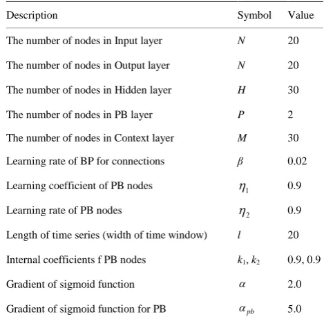
The proposed method was applied to a complex behavior learning and generation of a humanoid robot named “PALRO” (Fujisoft, Inc., 2010) as shown in Figure 2.

There are 20 joints (actuators) in PALRO (arms, legs, neck, and body) and the control of these angles of joints in time series composes various actions of the robot. Two kinds of experiments were designed:

[image:3.595.130.217.394.488.2]

Experiment I: a time series angles of joints yield a primitive behavior, such as raising a hand, or turning to left/right, and several primitive behaviors yield a complex

Figure 2. A robot used in the experiment: PALRO, product of Fujisoft, Inc., 2010.

(a) Pattern 1 (b) Pattern 2

(c) Pattern 3 (d) Pattern 4 Figure 3. Primitive behaviors of the robot in experiment I. behavior of the robot such as a “dance” behavior;

Experiment II: 3 kinds of voice instructions corres-ponding to 3 kinds of behaviors of robot were learned and recognized.

Details of the experiments and results were described in this section.

3.1.

Experiment I: Complex Behavior Learning

and Generation

3.1.1 Primitive Behavior Learning / Generation

We designed 4 kinds of patterns of primitive behaviors of the robot as shown in Figure 3: (a) Turn to left and shake the hands; (b) Turn to right and shake the hands; (c) Turn to right and shake the hands; (d) Raise the left hand and stop in a special pose. Angle vector with 20 dimensions served the input of RNNPB, that is, the number of nodes in Input layer and Output layer was 20 respectively. Teach signals of the primitive behaviors were recorded by the storage function of the robot, that is, the time series values of angles of the movements (pri-mitive behaviors) obtained by the drive of an instructor. Parameters of RNNPB and its learning process used in the experiment are listed in Table 1.

[image:3.595.304.539.477.708.2]

Training results of RNNPB for the 4 primitive beha-viors are shown in Figure 4, where (a) shows the learn-ing curve (Iteration time vs. RMSE); (b) PB values of the 4 patterns of behaviors; (c)-(f) time series values of 20 angles of behaviors (generation with 30% teacher signals). The time interval “step” was set with 0.1 second/step in (c)-(f).

Table 1. Parameters used in RNNPB in Experiment I.

Description Symbol Value

The number of nodes in Input layer N 20

The number of nodes in Output layer N 20 The number of nodes in Hidden layer H 30

The number of nodes in PB layer P 2

The number of nodes in Context layer M 30 Learning rate of BP for connections β 0.02

Learning coefficient of PB nodes η₁ 0.9

Learning rate of PB nodes η₂ 0.9

Length of time series (width of time window) l 20 Internal coefficients f PB nodes k1, k2 0.9, 0.9

Gradient of sigmoid function α 2.0

[image:3.595.66.281.528.689.2]

(4)

In fact, if the teacher signals were not added during the generation process, that is, the input signal was given by following equation:

) 1 ( ) 1 ( ) 1 ( )

(t = −r xt− +rxd t−

x (7)

where x(t-1) is the output of the network on time t-1,

xd(t-1) is the teacher data and r is the ratio of the teacher signal.

When r = 0.0, the output of the network was easily to fall in a static state and this problem needs to be im-proved in the future study.

3.1.2. Complex Behavior Learning / Generation

Using the Q-Learning algorithm (QL) described in last section, we decided the required orders of the primitive patterns to compose the complex behavior: a “dance” of robot.

The QL was defined with 4 states, that is, 4 values of PB nodes and 4 actions as same as these PB values. The training results gave the order of PB values used in the generation process of robot as follows:

“Pattern 3 - Pattern 1 – Pattern 2 – Pattern 3 – Pattern 4”.

The reward to reinforce the adaptive transition was

(a) Learning curve of RNNPB

Pattern 1 ＋ Pattern 2 × Pattern 3 ＊ Pattern 4 □

(b) PB values of 4 patterns

(c) Angles for Pattern 1

(d) Angles for Pattern 2

(e) Angles for Pattern 3

[image:4.595.322.525.94.710.2]

(f) Angles for Pattern 4

(5)

input by the voice of instructor. “Good” said by the in-structor indicated the value of reward R = 0.1, and “Bad” meant R = -0.1. Parameters used in the QL are listed in

Table 2. The learning curve (Iteration times vs. Success rate; 10 experiments averages) and final time series val-ues of angles of the complex behavior “dance” are shown in Figure 5. The success rate of the dance composed by the fixed order of primitive behaviors reached to 100.0% after 12 trials of QL.

The complex behavior generation movie is shown on the WWW site:

http://www.nn.csse.yamaguchi-u.ac.jp/images/researc h/Palro11Hashiguchi.wmv

Table 2. Parameters used in Q-Learning.

Learning rate of Q λ 0.1

Discount rate γ 0.9

Reward (positive / negative) R 0.1/ -0.1

Rate of random action ε 0.1

(a) Learning curve of QL

(b) Time series values of 20-joint angles to realize the “dance” as a composition of 4 primitive behaviors.

Figure 5. Leaning results of a complex behavior “dance”.

3.2.

Experiment II: Behavior Instruction

Learning and Recognition

Voice instruction can be captured and recognized by the recorder and microphone of PALRO. However, special behaviors need to be learned by the instructor and the learning system RNNPB, and the relationship between PB values and the voice instructions is able to be decided by QL algorithm as same as the situation of order decision of primitive behaviors for complex behavior learning and generation. In this experiment, we designed 3 kinds of behaviors for PALRO which static picture are shown in

Figure 6: (a) Shake a hand; (b) Raise 2 hands; (3) A handclap. Because the behaviors were limited in several joints, 8 input / output nodes were designed in RNNPB, and other parameters used in the experiment II are listed in Table 3. Parameters used in QL were as same as in the Experiment I (Table 2). Figure 7 shows the scene of teaching process where angles of 8 joints were changed by the instructor and they were recorded as a time series data as a teach signal of a behavior. The voice instruction learning and recognition results also achieved 100.0% of successful rate, and the details are omitted here for the limit of space.

(a) Raise a hand (b) Raise 2 hands (c) A handclap Figure 6. Leaning results of a complex behavior “dance”.

Table 3. Parameters used in RNNPB in Experiment II.

The number of nodes in Input layer N 8 The number of nodes in Output layer N 8 The number of nodes in Hidden layer H 20

The number of nodes in PB layer P 2

The number of nodes in Context layer M 30 Learning rate of BP for connections β 0.01 Learning coefficient of PB nodes η₁ 0.1

Learning rate of PB nodes η₂ 0.9

Length of time series

(width of time window) l 20

Internal coefficients f PB nodes k1, k2 0.8, 0.5

Gradient of sigmoid function α 2.0

(6)

[image:6.595.127.220.96.168.2]

Figure 7. Leaning results of a complex behavior “dance”.

4.

Conclusion

The combination of a recurrent neural network with bias parameters (RNNPB) and reinforcement learning algorithm was proposed to realize the complex behavior learning and generation of robot. All angles of joints of robot were considered as the input and output of RNNPB and their time series data formed kinds of patterns of primitive behaviors of robot at first, then the complex behavior of robot were composed by the time series of different primitive behaviors. The learning rule of RNNPB used error back propagation through time (BPTT) method, and to generate a series of primitive behaviors in correct order, Q-learning (QL) was adopt in the training process. Using a humanoid robot “PALRO”, the proposed method was confirmed its effectiveness by the results of two kinds of experiments. The generation of primitive behaviors showed a satisfied representation of required movement when a certain of teach signal was added during the generation process and a 100.0% of success rate of a complex behavior “dance” was acquired after the training with the QL algorithm. Voice instruction learning and recognition also reached to 100.0% success rate in the experiment.

5.

Acknowledgements

A part of this work was supported by Grant-in-Aid for Scientific Research (JSPS 23500181) and Foundation for the Fusion of Science and Technology (FOST).

REFERENCES

[1] V. I. Pavlovic, R. Sharma, and T. S. Huang, “Visual In-terpretation of Hand Gestures for Human-Computer Inte-raction: A Review”, IEEE Transaction on Pattern Analy-sis and Machine Learning Intelligence, Vol. 19, No. 7, 1997, pp. 667-695.

[2] C. Nolker, H. Ritter, Parametrized SOMs for hand post-ure reconstruction. Proceedings of IEEE-INNS-ENNS

International Joint Conference on Neural Networks (IJCNN’00), 2000, pp. 139—144.

[3] G. Heidemann, H. Bekel, I. Bax, A. Saalbach, Hand ges-ture recognition: selforganising maps as a graphical user interface for the partitioning of large training data sets, in:

Proceedings of 17th International Conference on Pattern

Recognition (ICPR’04), 2004, pp.487—490.

[4] C.-L. Huang, M.-S. Wu, S.-H. Jeng, Gesture recognition using the multi-PDM method and hidden Markov model,

Image and Vision Computing, Vol.18, No.11, 2000, pp.865–879.

[5] R. Amit and M. Mataric, “Learning Movement Se-quences from Demonstration”, Proceedings of the 2nd IEEE International Conference on Development and Learning (ICDL’02), Cambridge, MA, 2002, pp. 203-208.

[6] M. Hossain, M. Jenkin, Recognizing hand-raising gesture using HMM, in: Proceedings of 2nd Canadian Confe-rence on Computer and Robot Vision (CRV’05), 2005, pp.405-412.

[7] G. Caridakis, K. Karpouzis, A. Drosopoulos, S. Kollias, SOMM: Self Organizing Markov Map for Gesture Rec-ognition, Pattern Recognition Letters, Vol. 31, No.1, 2010, pp. 52-59.

[8] H. Suk, B. Sin and S. Lee, “Recognize Hand Gesture using Dynamic Baysian Network”, Proceedings of 8th IEEE international Conference on Automatic Face & Gesture Recognition (FG’08), 2008, pp. 1-6.

[9] J. Tani, “Learning to Generate Articulated Behavior through the Bottom-Up and the Top-Down Interaction Process”, Neural Networks, Vol. 16, 2003, pp. 11-23. [10] J. Tani and M. Ito, “Self-Organization of Behavioral

Pri-mitives as Multiple Attractor Dynamics: A Robot Expe-riment”, IEEE Transactions on Systems, Man, and Cy-bernetics, Vol. 33, No. 4, 2003, pp. 481-488.

[11] J. Tani, M. Ito and Y. Sugita, “Self-organization of Dis-tributedly Represented Multiple Behavior Schemata in a Mirror System: Reviews of Robot Experiments Using RNNPB”, Neural Networks, Vol.17, 2004, pp.1273-1289. [12] T. Kuremoto, Y. Kinoshita, L. B. Feng, S. Watanabe, K. Kobayashi, M. Obayashi, “A Gesture Recognition Sys-tem with Retina-V1 Model and One-Pass Dynamic Pro-gramming”, Neurocomputing, 2012, in press, doi: http://dx.doi.org/10/1016/j.neucom.2012.03.27

[13] G. rizzolatti and L. Craighero, “The MiNror-neuron Sys-tem”, Annual Reviews of Neuroscience, Vol. 27, 2004, pp. 169-192.

[14] E. Oztop, M. Kawato and M. Arbib, “Mirror Neurons and Imitation: A Computationally Guided View”, Neural Networks, Vol. 19, 2006, pp. 254-271.

[15] R. S. Sutton and A. G. Barto, “Reinforcement Learning: An introduction”, The MIT Press, Cambridge, 1998.

[16] J. L. Elman, “Finding Structure in Time”, Cognitive Science, Vol. 14, 1990, pp. 179-211.

[17] D. Rumelhart, G. E. Hinton and R. J. Williams, “Learn-ing Internal Representations by Back-Propagation Errors”,

Nature, Vol. 233, 1986, pp. 533-536.