Learning Character level Compositionality with Visual Features

Proceedings of the 55th Annual Meeting of the Association for Computational Linguistics, pages 2059–2068 Vancouver, Canada, July 30 - August 4, 2017. c2017 Association for Computational Linguistics Proceedings of the 55th Annual Meeting of the Association for Computational Linguistics, pages 2059–2068

Vancouver, Canada, July 30 - August 4, 2017. c2017 Association for Computational Linguistics

Learning Character-level Compositionality with Visual Features

Frederick Liu1_{, Han Lu}1_{, Chieh Lo}2_{, Graham Neubig}1

1_{Language Technology Institute} 2_{Electrical and Computer Engineering} Carnegie Mellon University, Pittsburgh, PA 15213

{fliu1,hlu2,gneubig_}@cs.cmu.edu [email protected]

Abstract

Previous work has modeled the composi-tionality of words by creating character-level models of meaning, reducing prob-lems of sparsity for rare words. However, in many writing systems compositionality has an effect even on the character-level: the meaning of a character is derived by the sum of its parts. In this paper, we model this effect by creating embeddings for characters based on their visual teristics, creating an image for the charac-ter and running it through a convolutional neural network to produce a visual char-acter embedding. Experiments on a text classification task demonstrate that such model allows for better processing of in-stances with rare characters in languages such as Chinese, Japanese, and Korean. Additionally, qualitative analyses demon-strate that our proposed model learns to focus on the parts of characters that carry semantic content, resulting in embeddings that are coherent in visual space.

1 Introduction

Compositionality—the fact that the meaning of a complex expression is determined by its structure and the meanings of its constituents—is a hall-mark of every natural language (Frege and Austin,

1980;Szab´o,2010). Recently, neural models have provided a powerful tool for learning how to com-pose words together into a meaning representation of whole sentences for many downstream tasks. This is done using models of various levels of sophistication, from simpler bag-of-words (Iyyer et al., 2015) and linear recurrent neural network (RNN) models (Sutskever et al.,2014;Kiros et al.,

2015), to more sophisticated models using

tree-K

a

lb

Kälber

a

Do Do'(polite)

Calf

Calves

Laurel

Whale

Salmon

Salmon

gui jing

gui gui

(a)

(b)

(c)

(d)

han'da ham''ni'''da

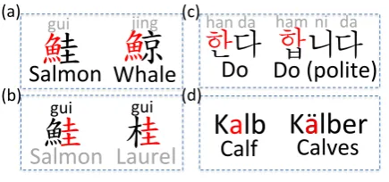
Figure 1: Examples of character-level composi-tionality in (a, b) Chinese, (c) Korean, and (d) Ger-man. The red part of the characters are shared, and affects the pronunciation (top) or meaning (bot-tom).

structured (Socher et al., 2013) or convolutional networks (Kalchbrenner et al.,2014).

In fact, a growing body of evidence shows that it is essential to look below the word-level and con-sider compositionality within words themselves. For example, several works have proposed mod-els that represent words by composing together the characters into a representation of the word it-self (Ling et al.,2015;Zhang et al.,2015;Dhingra et al.,2016). Additionally, for languages with pro-ductive word formation (such as agglutination and compounding), models calculating morphology-sensitive word representations have been found ef-fective (Luong et al., 2013;Botha and Blunsom,

2014). These models help to learn more robust representations forrare wordsby exploiting mor-phological patterns, as opposed to models that op-erate purely on the lexical level as the atomic units. For many languages, compositionality stops at the character-level: characters are atomic units of meaning or pronunciation in the language, and no further decomposition can be done.1 _{However, for} other languages, character-level compositionality, where a character’s meaning or pronunciation can

1_{In English, for example, this is largely the case.}

Lang Geography Sports Arts Military Economics Transportation

Chinese 32.4k 49.8k 50.4k 3.6k 82.5k 40.4k

Japanese 18.6k 82.7k 84.1k 81.6k 80.9k 91.8k

Korean 6k 580 5.74k 840 5.78k 1.68k

Lang Medical Education Food Religion Agriculture Electronics

Chinese 30.3k 66.2k 554 66.9k 89.5k 80.5k

Japanese 66.5k 86.7k 20.2k 98.1k 97.4k 1.08k

Korean 16.1k 4.71k 33 2.60k 1.51k 1.03k

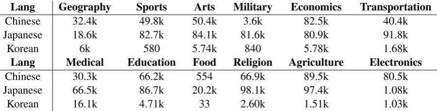
Table 1: By-category statistics for the Wikipedia dataset. Note that Food is the abbreviation for “Food and Culture” and Religion is the abbreviation for “Religion and Belief”.

be derived from the sum of its parts, is very much a reality. Perhaps the most compelling example of compositionality of sub-character units can be found in logographic writing systems such as the Han and Kanji characters used in Chinese and Japanese, respectively.2 _{As shown on the left side} of Fig.1, each part of a Chinese character (called a “radical”) potentially contributes to the meaning (i.e., Fig. 1(a)) or pronunciation (i.e., Fig. 1(b)) of the overall character. This is similar to how English characters combine into the meaning or pronunciation of an English word. Even in lan-guages with phonemic orthographies, where each character corresponds to a pronunciation instead of a meaning, there are cases where composition occurs. Fig.1(c) and (d) show the examples of Ko-rean and German, respectively, where morpholog-ical inflection can cause single characters to make changes where some but not all of the component parts are shared.

In this paper, we investigate the feasibility of modeling thecompositionality of characters in a way similar to how humans do: by visually ob-serving the character and using the features of its shape to learn a representation encoding its mean-ing. Our method is relatively simple, and gener-alizable to a wide variety of languages: we first transform each character from its Unicode repre-sentation to a rendering of its shape as an image, then calculate a representation of the image us-ing Convolutional Neural Networks (CNNs) (Cun et al., 1990). These features then serve as inputs to a down-stream processing task and trained in an end-to-end manner, which first calculates a loss function, then back-propagates the loss back to the CNN.

2_{Other prominent examples are largely for extinct}

lan-guages: Egyptian hieroglyphics, Mayan glyphs, and Sume-rian cuneiform scripts (Daniels and Bright,1996).

As demonstrated by our motivating examples in Fig.1, in logographic languages character-level semantic or phonetic similarity is often indicated by visual cues; we conjecture that CNNs can appropriately model these visual patterns. Con-sequently, characters with similar visual appear-ances will be biased to have similar embeddings, allowing our model to handlerare characters ef-fectively, just as character-level models have been effective for rare words.

To evaluate our model’s ability to learn repre-sentations, particularly for rare characters, we per-form experiments on a downstream task of classi-fying Wikipedia titles for three Asian languages: Chinese, Japanese, and Korean. We show that our proposed framework outperforms a baseline model that uses standard character embeddings for instances containing rare characters. A qualita-tive analysis of the characteristics of the learned embeddings of our model demonstrates that visu-ally similar characters share similar embeddings. We also show that the learned representations are particularly effective under low-resource scenar-ios and complementary with standard character embeddings; combining the two representations through three different fusion methods (Snoek et al., 2005;Karpathy et al., 2014) leads to con-sistent improvements over the strongest baseline without visual features.

2 Dataset

com-100 ₁₀1 ₁₀2 ₁₀3 ₁₀4

106

100

101

102

103

104

105

Rank

Frequency

⎯⎯

⎯⎯

"

⎯⎯

Rank < 20% Freq. > 80%

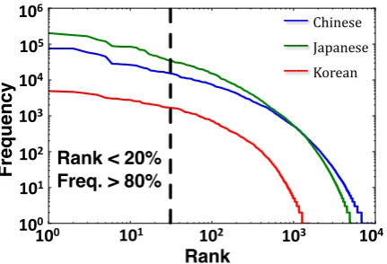
Figure 2: The character rank-frequency distribu-tion of the corpora we considered in this paper. All three languages have a long-tail distribution.

positionality in the characters of the language. To satisfy these desiderata, we create a text classifi-cation dataset where the input is a Wikipedia ar-ticle title in Chinese, Japanese, or Korean, and the output is the category to which the article be-longs.3_{This satisfies (1), because Wikipedia titles} are short and thus each character in the title will be important to our decision about its category. It also satisfies (2), because Chinese, Japanese, and Korean have writing systems with large numbers of characters that decompose regularly as shown in Fig.1. While this task in itself is novel, it is similar to previous work in named entity type in-ference using Wikipedia (Toral and Munoz,2006;

Kazama and Torisawa, 2007; Ratinov and Roth,

2009), which has proven useful for downstream named entity recognition systems.

2.1 Dataset Collection

As the labels we would like to predict, we use 12 different main categories from the Wikipedia web page: Geography, Sports, Arts, Military, Eco-nomics, Transportation, Health Science, Educa-tion, Food Culture, Religion and Belief, Agricul-ture and Electronics. Wikipedia has a hierarchical structure, where each of these main categories has a number of subcategories, and each subcategory has its own subcategories, etc. We traverse this hierarchical structure, adding each main category tag to all of its descendants in this subcategory tree structure. In the case that a particular article is the descendant of multiple main categories, we favor the main category that minimizes the depth of the 3_{The link to the dataset and the crawling scripts}

– https://github.com/frederick0329/ Wikipedia_title_dataset

Geography Sports Arts Military Economics Transportation Health Science Education Food Culture Religion and Belief Agriculture Electronics Visual model

(Image as input)

Lookup model (Symbol as input)

CNN CNN CNN

Softmax GRU

36 36

Figure 3: An illustration of two models, our pro-posed VISUAL model at the top and the

base-line LOOKUPmodel at the bottom using the same

RNN architecture. A string of characters (e.g. “温

病学_{”), each converted into a 36x36 image, serves}

as input of our VISUAL model. dc is the

dimen-sion of the character embedding for the LOOKUP

model.

article in the tree (e.g., if an article is two steps away from Sports and three steps away from Arts, it will receive the “Sports” label). We also per-form some rudimentary filtering, removing pages that match the regular expression “.*:.*”, which catches special pages such as “title:agriculture”.

2.2 Statistics

For Chinese, Japanese, and Korean, respectively, the number of articles is 593k/810k/46.6k, and the average length and standard deviation of the ti-tle is 6.25±3.96/8.60±5.58/6.10±3.71. As shown in Fig. 2, the character rank-frequency distribu-tions of all three languages follows the 80/20 rule (Newman,2005) (i.e., top 20% ranked char-acters that appear more than 80% of total frequen-cies), demonstrating that the characters in these languages belong to a long tail distribution.

We further split the dataset into training, valida-tion, and testing sets with a 6:2:2 ratio. The cat-egory distribution for each language can be seen in Tab.1. Chinese has two varieties of characters, traditional and simplified, and the dataset is a mix of the two. Hence, we transform this dataset into two separate sets, one completely simplified and the other completely traditional using the Chinese text converter provided with Mac OS.

3 Model

Layer# 3-layer CNN Configuration

1 Spatial Convolution (3, 3)→32

2 ReLu

3 MaxPool (2, 2)

4 Spatial Convolution (3, 3)→32

5 ReLu

6 MaxPool (2, 2)

7 Spatial Convolution (3, 3)→32

8 ReLu

9 Linear (800, 128)

10 ReLu

11 Linear (128, 128)

12 ReLu

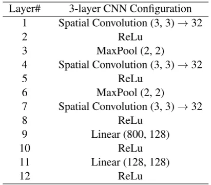
Table 2: Architecture of the CNN used in the ex-periments. All the convolutional layers have 32 3×3 filters.

We calculate character representations, use a RNN to combine the character representations into a sentence representation, and then add a softmax layer after that to predict the probability for each class. As shown in Fig. 2.1, the baseline model, which we call it the LOOKUP model, calculates

the representation for each character by looking it up in a character embedding matrix. Our proposed model, the VISUAL model instead learns the

rep-resentation of each character from its visual ap-pearance via CNN.

LOOKUP model Given a character vocabulary C, for the LOOKUPmodel as in the bottom part of

Fig. 2.1, the input to the network is a stream of charactersc1, c2, ...cN, wherecn∈C. Each

char-acter is represented by a 1-of-|C| (one-hot) en-coding. This one-hot vector is then multiplied by the lookup matrixTC ∈ R|C|×dc, wheredcis the

dimension of the character embedding. The ran-domly initialized character embeddings were opti-mized with classification loss.

VISUAL model The proposed method aims to

learn a representation that includes image in-formation, allowing for better parameter sharing among characters, particularly characters that are less common. Different from the LOOKUPmodel,

each character is first transformed into a 36-by-36 image based on its Unicode encoding as shown in the upper part of Fig 2.1. We then pass the im-age through a CNN to get the embedding for the image. The parameters for the CNN are learned through backpropagation from the classification

loss. Because we are training embeddings based on this classification loss, we expect that the CNN will focus on parts of the image that contain se-mantic information useful for category classifica-tion, a hypothesis that we examine in the experi-ments (see Section5.5).

In more detail, the specific structure of the CNN that we utilize consists of three convolution layers where each convolution layer is followed by the max pooling and ReLU nonlinear activation lay-ers. The configurations of each layer are listed in Tab.2. The output vector for the image embed-dings also has size dc which is the same as the

LOOKUPmodel.

Encoder and Classifier For both the

LOOKUP and the VISUAL models, we adopt

an RNN encoder using Gated Recurrent Units (GRUs) (Chung et al., 2014). Each of the GRU units processes the character embeddings sequen-tially. At the end of the sequence, the incremental GRU computation results in a hidden state e embedding the sentence. The encoded sentence embedding is passed through a linear layer whose output is the same size as the number of classes. We use a softmax layer to compute the posterior class probabilities:

P(y=j|e) = exp(w

T

je+bj)

PL

i=1exp(wiTe+bi)

(1)

To train the model, we use cross-entropy loss between predicted and true targets:

J = 1

B

B X

i=1 L X

j=1

−ti,jlog(pi,j) (2)

whereti,j ∈ {0,1}represents the ground truth

la-bel of thej-th class in thei-th Wikipedia page ti-tle. B is the batch size and L is the number of categories.

4 Fusion-based Models

One thing to note is that the LOOKUP and the

VISUAL models have their own advantages. The

LOOKUP model learns embedding that captures

the semantics of each character symbol without sharing information with each other. In con-trast, the proposed VISUALmodel directly learns

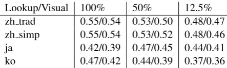
Lookup/Visual 100% 50% 12.5%

zh trad 0.55/0.54 0.53/0.50 0.48/0.47

zh simp 0.55/0.54 0.53/0.52 0.48/0.46

ja 0.42/0.39 0.47/0.45 0.44/0.41

ko 0.47/0.42 0.44/0.39 0.37/0.36

Table 3: The classification results of the LOOKUP

/ VISUALmodels for different percentages of full

training size.

model the ability to generalize better to rare char-acters, but also has the potential disadvantage of introducing noise for characters with similar ap-pearances but different meanings.

With the complementary nature of these two models in mind, we further combine the two em-beddings to achieve better performances. We adopt three fusion schemes, early fusion, late fu-sion (described bySnoek et al.(2005) and Karpa-thy et al. (2014)), and fallback fusion, a method specific to this paper.

Early Fusion Early fusion works by concatenat-ing the two varieties of embeddconcatenat-ings before feedconcatenat-ing them into the RNN. In order to ensure that the di-mensions of the RNN are the same after concate-nation, the concatenated vector is fed through a hidden layer to reduce the size from2_×dctodc.

The whole model is then fine-tuned with training data.

Late Fusion Instead of learning a joint represen-tation like early fusion, late fusion averages the model predictions. Specifically, it takes the output of the softmax layers from both models and aver-ages the probabilities to create a final distribution used to make the prediction.

Fallback Fusion Our final fallback fusion

method hypothesizes that our VISUALmodel does

better with instances which contain more rare characters. First, in order to quantify the over-all rareness of an instance consisting of multiple characters, we calculate the average training set frequency of the characters therein. The fallback fusion method uses the VISUAL model to predict

testing instances with average character frequency below or equal to a threshold (here we use 0.0 fre-quency as cutoff, which means all characters in the instance do not appear in the training set), and uses the LOOKUP model to predict the rest of the

in-stances.

5 Experiments and Results

In this section, we compare our proposed VISUAL

model with the baseline LOOKUP model through

three different sets of experiments. First, we ex-amine whether our model is capable of classify-ing text and achievclassify-ing similar performance as the baseline model. Next, we examine the hypothesis that our model will outperform the baseline model when dealing with low frequency characters. Fi-nally, we examine the fusion methods described in Section4.

5.1 Experimental Configurations

The dimension of the embeddings and batch size for both models are set to dc = 128 and B =

400, respectively. We build our proposed model

using Torch (Collobert et al.,2002), and use Adam (Kingma and Ba,2014) with a learning rateη = 0.001for stochastic optimization. The length of

each instance is cut off or padded to 10 characters for batch training.

5.2 Comparison with the Baseline Model In this experiment, we examine whether our VI -SUAL model achieves similar performance with

the baseline LOOKUP model in classification

ac-curacy.

The results in Tab. 3 show that the baseline model performs 1-2% better across four datasets; this is due to the fact that the LOOKUPmodel can

directly learn character embeddings that capture the semantics of each character symbol for fre-quent characters. In contrast, the VISUAL model

learns embeddings from visual information, which constraints characters that has similar appearance to have similar embeddings. This is an advantage for rare characters, but a disadvantage for high fre-quency characters because being similar in appear-ance does not always lead to similar semantics.

To demonstrate that this is in fact the case, be-sides looking at the overall classification accuracy, we also examine the performance on classifying low frequency instances which are sorted accord-ing to the average trainaccord-ing set frequency of the characters therein. Tab.4and Fig.4both show that our model performs better in the 100 lowest fre-quency instances (the intersection point of the two models). More specifically, take Fig.4(a)’ as ex-ample, the solid (proposed) line is higher than the dashed (baseline) line up to102, indicating that the

101 102 103 100

101 102 103

102 103

100 101 102 103

102 103

100 101 102 103

102 103

100 101 102 103

A

c

c

u

m

u

la

te

d

N

u

m

b

e

r

o

f

C

o

rr

e

c

tl

y

Pr

e

d

ic

te

d

I

n

s

ta

n

c

e

s

Rank

(a) (b)

(c) _(d)

⎯⎯!Visual,(TP(=(100%

⎯⎯!Visual,(TP(=(50%

⎯⎯!Visual,(TP(=(12.5%

⎯!⎯!Lookup,(TP(=(100% ⎯!⎯!Lookup,(TP(=(50%

⎯!⎯!Lookup,(TP(=(12.5%

⎯⎯!Visual,(TP(=(100%

⎯⎯!Visual,(TP(=(50%

⎯⎯!Visual,(TP(=(12.5%

⎯!⎯!Lookup,(TP(=(100% ⎯!⎯!Lookup,(TP(=(50%

⎯!⎯!Lookup,(TP(=(12.5%

⎯⎯!Visual,(TP(=(100%

⎯⎯!Visual,(TP(=(50%

⎯⎯!Visual,(TP(=(12.5%

⎯!⎯!Lookup,(TP(=(100% ⎯!⎯!Lookup,(TP(=(50%

⎯!⎯!Lookup,(TP(=(12.5%

⎯⎯!Visual,(TP(=(100%

⎯⎯!Visual,(TP(=(50%

⎯⎯!Visual,(TP(=(12.5%

⎯!⎯!Lookup,(TP(=(100% ⎯!⎯!Lookup,(TP(=(50%

⎯!⎯!Lookup,(TP(=(12.5%

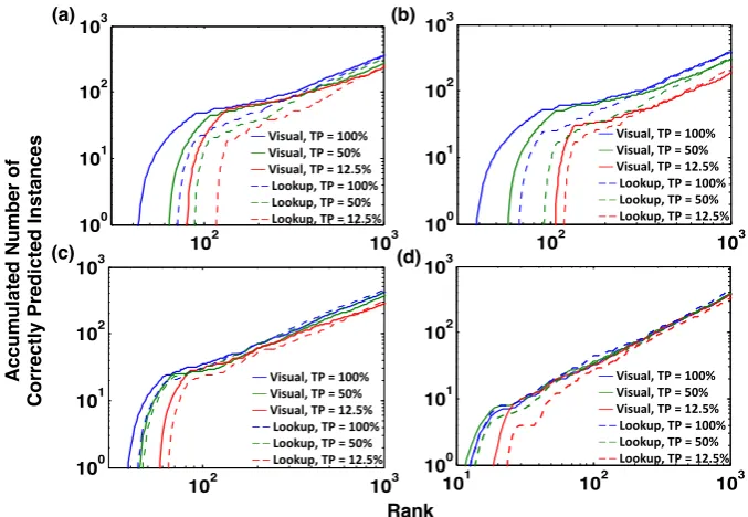
Figure 4: Experiments on different training sizes for four different datasets. More specifically, we con-sider three different training data size percentages (TPs) (100%, 50%, and 12.5%) and four datasets: (a) traditional Chinese, (b) simplified Chinese, (c) Japanese, and (d) Korean. We calculate the accumulated number of correctly predicted instances for the VISUAL model (solid lines) and the LOOKUP model

(dashed lines). This figure is a log-log plot, where x-axis shows rarity (rarest to the left), y-axis shows cumulative correctly classified instances up to this rank; a perfect classifier will result in a diagonal line.

first 100 instances. Lines depart the x-axis when the model classifies its first instance correctly, and the LOOKUPmodel did not correctly classify any

of the first 80 rarest instances, resulting in it cross-ing later than the proposed model. This confirms that the VISUAL model can share visual

informa-tion among characters and help to classify low fre-quency instances.

For training time, visual features take signifi-cantly more time, as expected. VISUAL is 30x slower than LOOKUP, although they are equiv-alent at test time. For space, images of Chinese characters took 36MB to store for 8985 characters.

5.3 Experiments on Different Training Sizes In our second experiment, we consider two smaller training sizes (i.e., 50% and 12.5% of the full training size) indicated by green and red lines in Fig. 4. We performed this experiment under the hypothesis that because the proposed method was more robust to infrequent characters, the proposed model may perform better in low-resourced sce-narios. If this is the case, the intersection point of the two models will shift right because of the in-crease of the number of instances with low average character frequency.

Lookup/Visual 100 1000 10000

zh trad 0.22/0.49 0.35/0.35 0.40/0.39

zh simp 0.25/0.53 0.39/0.37 0.41/0.40

ja 0.30/0.35 0.45/0.41 0.44/0.41

ko 0.44/0.33 0.44/0.33 0.48/0.42

Table 4: Classification results for the LOOKUP

/ VISUAL of the k lowest frequency instances across four datasets. The 100 lowest frequency in-stances for traditional and simplified Chinese and Korean were both significant (p-value < 0.05). Those for Japanese were not (p-value = 0.13); likely because there was less variety than Chinese and more data than Korean.

As we can see in Fig.4, the intersection point for 100% training data lies between the intersec-tion point for 50% training data and 12.5%. This disagrees with our hypothesis; this is likely be-cause while the number of low-frequency charac-ters increases, smaller amounts of data also ad-versely impact the ability of CNN to learn useful visual features, and thus there is not a clear gain nor loss when using the proposed method.

char-zh trad char-zh simp ja ko

Lookup 0.5503 0.5543 0.4914 0.4765

Visual 0.5434 0.5403 0.4775 0.4207

early 0.5520 0.5546 0.4896 0.4796

late 0.5658 0.5685 0.5029 0.4869

fall 0.5507 0.5547 0.4914 0.4766

Table 5: Experiment results for three different fu-sion methods across 4 datasets. The late fufu-sion model was better (p-value < 0.001) across four datasets.

acters in the test set, we use traditional Chinese as our training data and simplified Chinese as our testing data. The model was able to achieve around 40% classification accuracy when we use the full training set, compared to 55%, which is achieved by the model trained on simplified Chi-nese. This result demonstrates that the model is able to transfer between similar scripts, similarly to how most Chinese speakers can guess the mean-ing of the text, even if it is written in the other script.

5.4 Experiment on Different Fusion Methods Results of different fusion methods can be found in Tab. 5. The results show that late fusion gives the best performance among all the

fu-sion schemes combining the LOOKUP model

and the proposed VISUAL model. Early fusion

achieves small improvements for all languages ex-cept Japanese, where it displays a slight drop. Unsurprisingly, fallback fusion performs better than the LOOKUP model and the VISUAL model

alone, since it directly targets the weakness of the LOOKUPmodel (e.g., rare characters) and replaces

the results with the VISUAL model. These

re-sults show that simple integration, no matter which schemes we use, is beneficial, demonstrating that both methods are capturing complementary infor-mation.

5.5 Visualization of Character Embeddings Finally, we qualitatively examine what is learned by our proposed model in two ways. First, we visualize which parts of the image are most im-portant to the VISUALmodel’s embedding

calcu-lation. Second, we show the 6-nearest neighbor results for characters using both the LOOKUPand

the VISUALembeddings.

Iron Bronze Salmon Serranidae

Silk Coil Rhyme Pleased

Wave Put on Cypress Pillar

Cuckoo Eagle Mosquito Ant

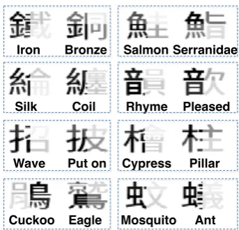
Figure 5: Examples of how much each part of the character contributes to its embedding (the darker the more). Two characters are shown per radical to emphasize that characters with same radical have similar patterns.

Emphasis of the VISUAL Model In order to

delve deeper into what the VISUAL model has

learned, we measure a modified version of the oc-clusion sensitivity proposed byZeiler and Fergus

(2014) by masking the original character image in four ways, and examine the importance of each part of the character to the model’s calculated rep-resentations. Specifically, we leave only the up-per half, bottom half, left half, or right half of the image, and mask the remainder with white pix-els since Chinese characters are usually formed by combining two radicals vertically or horizon-tally. We run these four images forward through the CNN part of the model and calculate the L2

distance between the masked image embeddings with the full image embedding. The larger the dis-tance, the more the masked part of the character contributes to the original embedding. The contri-bution of each part (e.g. theL2 distance) is

repre-sented as a heat map, and then it is normalized to adjust the opacity of the character strokes for bet-ter visualization. The value of each corner of the heatmap is calculated by adding the two L2

dis-tances that contribute to this corner.

! ! !

!!

!

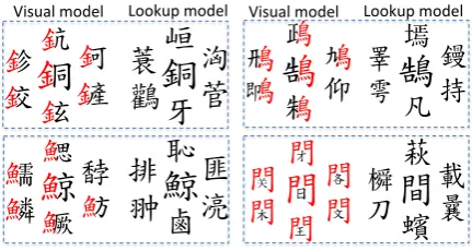
Visual'model Lookup'model Visual'model Lookup'model

Figure 6: Visualization of the Chinese traditional characters by finding the 6-nearest neighbors of the query (i.e., center) characters. The highlighted red indicates the radical along with the meaning of the characters.

highlighted in both “鐵_{” (Iron) and “}銅_{” (Bronze).}

We can also find similar results for other exam-ples shown in Fig. 5. Fig. 5 also demonstrated that our model captures the compositionality of Chinese characters, both meaning of sub-character units and their structure (e.g. the semantic content tends to be structurally localized on one side of a Chinese character).

K-nearest neighbors Finally, to illustrate the difference of the learned embeddings between the two models, we display 6-nearest neighbors (L2

distance) for selected characters in Fig.6. As can be seen, the VISUAL embedding for characters

with similar appearances are close to each other. In addition, similarity in the radical part indicates semantic similarity between the characters. For example, the characters with radical “鳥_{” all refer}

to different type of birds.

The LOOKUPembedding do not show such

fea-ture, as it learns the embedding individually for each symbol and relies heavily on the training set and the task. In fact, the characters shown in Fig.6

for the LOOKUP model do not exhibit semantic

similarity either. There are two potential expla-nations for this: First, the category classification task that we utilized do not rely heavily on the fine-grained semantics of each character, and thus the LOOKUPmodel was able to perform well without

exactly capturing the semantics of each character precisely. Second, the Wikipedia dataset contains a large number of names and location and the char-acters therein might not have the same semantic meaning used in daily vocabulary.

6 Related Work

Methods that utilize neural networks to learn distributed representations of words or charac-ters have been widely developed. However, word2vec (Mikolov et al.,2013), for example, re-quires storing an extremely large table of vectors for all word types. For example, due to the size of word types in twitter tweets, work has been done to generate vector representations of tweets at character-level (Dhingra et al.,2016).

There is also work done in understanding math-ematical expressions with a convolutional net-work for text and layout recognition by using an attention-based neural machine translation sys-tem (Deng et al., 2016). They tested on real-world rendered mathematical expressions paired with LaTeX markup and show the system is ef-fective at generating accurate markup. Other than that, there are several works that combine visual information with text in improving machine trans-lation (Sutskever et al.,2014), visual question an-swering, caption generation (Xu et al.,2015), etc. These works extract image representations from a pre-trained CNN (Zhu et al., 2016; Wang et al.,

2016).

Unrelated to images, CNNs have also been used for text classification (Kim, 2014; Zhang et al.,

2015). These models look at the sequential depen-dencies at the word or character-level and achieve the state-of-the-art results. These works inspire us to use CNN to extract features from image and serve as the input to the RNN. Our model is able to directly back-propagate the gradient all the way through the CNN, which generates visual embed-dings, in a way such that the embedding can con-tain both semantic and visual information.

Several techniques for reducing the rare words effects have been introduced in the literature, in-cluding spelling expansion (Habash,2008), dictio-nary term expansion (Habash,2008), proper name transliteration (Daum´e and Jagarlamudi, 2011), treating words as a sequence of characters ( Lu-ong and Manning,2016), subword units (Sennrich et al., 2015), and reading text as bytes (Gillick et al., 2015). However, most of these techniques still have no mechanism for handling low fre-quency characters, which are the target of this work.

of what radicals are included in which characters (Li et al.,2015;Shi et al.,2015;Yin et al.,2016). The motivation of this method is similar to ours, but is only applicable to Chinese, in contrast to the method in this paper, which works on any lan-guage for which we can render text.

7 Conclusion and Future Work

In this paper, we proposed a new framework that utilizes appearance of characters, convolu-tional neural networks, recurrent neural networks to learn embeddings that are compositional in the component parts of the characters. More specif-ically, we collected a Wikipedia dataset, which consists of short titles of three different languages and satisfies the compositionality in the characters of the language. Next, we proposed an end-to-end model that learns visual embeddings for characters using CNN and showed that the features extracted from the CNN include both visual and semantic information. Furthermore, we showed that our VISUALmodel outperforms the LOOKUPbaseline

model in low frequency instances. Additionally, by examining the character embeddings visually, we found that our VISUAL model is able to learn

visually related embeddings.

In summary, we tackled the problem of rare characters by using embeddings learned from im-ages. In the future, we hope to further general-ize this method to other tasks such as pronuncia-tion estimapronuncia-tion, which can take advantage of the fact that pronunciation information is encoded in parts of the characters as demonstrated in Fig.1, or machine translation, which could benefit from a wholistic view that considers both semantics and pronunciation. We also hope to apply the model to other languages with complicated compositional writing systems, potentially including historical texts such as hieroglyphics or cuneiform.

Acknowledgments

We thank Taylor Berg-Kirkpatrick, Adhiguna Kuncoro, Chen-Hsuan Lin, Wei-Cheng Chang, Wei-Ning Hsu and the anonymous reviewers for their enlightening comments and feedbacks.

References

Jan A Botha and Phil Blunsom. 2014. Compositional morphology for word representations and language modelling. InICML. pages 1899–1907.

Junyoung Chung, Caglar Gulcehre, KyungHyun Cho, and Yoshua Bengio. 2014. Empirical evaluation of gated recurrent neural networks on sequence model-ing.arXiv preprint arXiv:1412.3555.

Ronan Collobert, Samy Bengio, and Johnny Marithoz. 2002. Torch: A modular machine learning software library.

Y. Le Cun, B. Boser, J. S. Denker, R. E. Howard, W. Habbard, L. D. Jackel, and D. Henderson. 1990. Advances in neural information processing systems 2. pages 396–404.

Peter T Daniels and William Bright. 1996.The world’s writing systems. Oxford University Press.

Hal Daum´e and Jagadeesh Jagarlamudi. 2011. Domain adaptation for machine translation by mining unseen words. InACL-HLT. pages 407–412.

Yuntian Deng, Anssi Kanervisto, and Alexander M. Rush. 2016. What you get is what you see: A visual markup decompiler. arXiv preprint arXiv:1609.04938.

Bhuwan Dhingra, Zhong Zhou, Dylan Fitzpatrick, Michael Muehl, and William W Cohen. 2016. Tweet2vec: Character-based distributed representa-tions for social media.ACL.

Gottlob Frege and John Langshaw Austin. 1980. The foundations of arithmetic: A logico-mathematical enquiry into the concept of number. Northwestern University Press.

Dan Gillick, Cliff Brunk, Oriol Vinyals, and Amarnag Subramanya. 2015. Multilingual language process-ing from bytes. arXiv preprint arXiv:1512.00103. Nizar Habash. 2008. Four techniques for online

han-dling of out-of-vocabulary words in Arabic-English statistical machine translation. InHLT-Short. pages 57–60.

Mohit Iyyer, Varun Manjunatha, and Jordan L Boyd-Graber. 2015. Deep unordered composition rivals syntactic methods for text classification. InACL. Nal Kalchbrenner, Edward Grefenstette, and Phil

Blun-som. 2014. A convolutional neural network for modelling sentences. ACLpages 655–665.

Andrej Karpathy, George Toderici, Sanketh Shetty, Thomas Leung, Rahul Sukthankar, and Li Fei-Fei. 2014. Large-scale video classification with convolu-tional neural networks. InCVPR. pages 1725–1732. Jun’ichi Kazama and Kentaro Torisawa. 2007. Ex-ploiting Wikipedia as external knowledge for named entity recognition. InEMNLP-CoNLL. pages 698– 707.

Diederik Kingma and Jimmy Ba. 2014. Adam: A method for stochastic optimization. arXiv preprint arXiv:1412.6980.

Ryan Kiros, Yukun Zhu, Ruslan R Salakhutdinov, Richard Zemel, Raquel Urtasun, Antonio Torralba, and Sanja Fidler. 2015. Skip-thought vectors. In NIPS. pages 3294–3302.

Yanran Li, Wenjie Li, Fei Sun, and Sujian Li. 2015. Component-enhanced chinese character em-beddings.EMNLPpages 829–834.

Wang Ling, Chris Dyer, Alan W Black, Isabel Tran-coso, Ramon Fermandez, Silvio Amir, Luis Marujo, and Tiago Luis. 2015. Finding function in form: Compositional character models for open vocabu-lary word representation. InEMNLP. pages 1520– 1530.

Minh-Thang Luong and Christopher D Manning. 2016. Achieving open vocabulary neural machine transla-tion with hybrid word-character models. ACLpages 1054–1063.

Thang Luong, Richard Socher, and Christopher Man-ning. 2013. Better word representations with recur-sive neural networks for morphology. In CoNLL. pages 104–113.

Tomas Mikolov, Ilya Sutskever, Kai Chen, Greg S Cor-rado, and Jeff Dean. 2013. Distributed representa-tions of words and phrases and their compositional-ity. InNIPS. pages 3111–3119.

Mej Newman. 2005. Power laws, Pareto distributions and Zipf’s law.CONTEMP PHYSpages 323–351. Lev Ratinov and Dan Roth. 2009. Design challenges

and misconceptions in named entity recognition. In CoNLL. pages 147–155.

Rico Sennrich, Barry Haddow, and Alexandra Birch. 2015. Neural machine translation of rare words with subword units. ACLpages 1715–1725.

Xinlei Shi, Junjie Zhai, Xudong Yang, Zehua Xie, and Chao Liu. 2015. Radical embedding: Delving deeper to chinese radicals. InACL. pages 594–598. Cees GM Snoek, Marcel Worring, and Arnold WM

Smeulders. 2005. Early versus late fusion in seman-tic video analysis. InACM MM. pages 399–402. Richard Socher, Alex Perelygin, Jean Y Wu, Jason

Chuang, Christopher D Manning, Andrew Y Ng, and Christopher Potts. 2013. Recursive deep mod-els for semantic compositionality over a sentiment treebank. InEMNLP. pages 1631–1642.

Ilya Sutskever, Oriol Vinyals, and Quoc V Le. 2014. Sequence to sequence learning with neural net-works. InNIPS. pages 3104–3112.

Zolt´an Gendler Szab´o. 2010. Compositionality. Stan-ford encyclopedia of philosophy.

Antonio Toral and Rafael Munoz. 2006. A proposal to automatically build and maintain gazetteers for named entity recognition by using wikipedia. In EACL. pages 56–61.

Jiang Wang, Yi Yang, Junhua Mao, Zhiheng Huang, Chang Huang, and Wei Xu. 2016. Cnn-rnn: A uni-fied framework for multi-label image classification. InCVPR. pages 2285–2294.

Kelvin Xu, Jimmy Ba, Ryan Kiros, Kyunghyun Cho, Aaron C Courville, Ruslan Salakhutdinov, Richard S Zemel, and Yoshua Bengio. 2015. Show, attend and tell: Neural image caption generation with visual at-tention. InICML.

Rongchao Yin, Quan Wang, Rui Li, Peng Li, and Bin Wang. 2016. Multi-granularity chinese word em-bedding. EMNLPpages 981–986.

Matthew D Zeiler and Rob Fergus. 2014. Visualiz-ing and understandVisualiz-ing convolutional networks. In ECCV. Springer, pages 818–833.

Xiang Zhang, Junbo Zhao, and Yann LeCun. 2015. Character-level convolutional networks for text clas-sification. InNIPS. pages 649–657.