Munich Personal RePEc Archive
Estimating Difference-in-Differences in
the Presence of Spillovers
Clarke, Damian
Universidad de Santiago de Chile
September 2017
Estimating Difference-in-Differences in the Presence of
Spillovers
∗
Damian Clarke
September 14, 2017
Abstract
I propose a method for difference-in-differences (DD) estimation in situations where the stable
unit treatment value assumption is violated locally. This is relevant for a wide variety of cases where spillovers may occur between quasi-treatment and quasi-control areas in a (natural) experiment. A
flexible methodology is described to test for such spillovers, and to consistently estimate treatment effects in their presence. This spillover-robust DD method results in two classes of estimands:
treat-ment effects, and “close” to treattreat-ment effects. The methodology outlined describes a versatile and non-arbitrary procedure to determine the distance over which treatments propagate, where distance can be defined in many ways, including as a multi-dimensional measure. This methodology is
illus-trated by simulation, and by its application to estimates of the impact of state-level text-messaging bans on fatal vehicle accidents. Extending existing DD estimates, I document that reforms travel
over roads, and have spillover effects in neighbouring non-affected counties. Text messaging laws appear to continue to alter driving behaviour as much as 30 km outside of affected jurisdictions.
JEL codes: C13, C21, D04, R23, K42.
Keywords: Policy evaluation, difference-in-differences, spillovers, natural experiments, SUTVA
∗I thank Serafima Chirkova, Paul Devereux, James Fenske, Rossa O’Keeffe-O’Donovan, Rudi Rocha, Chris Roth and
1
Introduction
Natural experiments often rely on territorial borders to estimate treatment effects. These borders sepa-rate quasi-treatment from quasi-control groups with individuals in one area having access to a program or treatment while those in another do not. In cases such as these where geographic location is used
to motivate identification, the stable unit treatment value assumption (SUTVA) is, either explicitly or implicitly, invoked.1
However, often territorial borders are porous. Generally state, regional, municipal, and village boundaries can be easily, if not costlessly, crossed. Given this, researchers interested in using natu-ral experiments in this way may be concerned that the effects of a program in a treatment cluster may spillover into non-treatment clusters—at least locally.
Such a situation is in clear violation of the SUTVA’s requirement that the treatment status of any one unit must not affect the outcomes of any other unit. In this paper I propose a methodology to deal with such spillover effects. I discuss how to test for local spillovers, and if such spillovers exist, how to estimate unbiased treatment effects in their presence. It is shown that this estimation requires a weaker condition than SUTVA: namely that SUTVA holds betweensomeunits, as determined by their distance from the treatment cluster. I discuss how to estimate treatment and spillover effects, and then
propose a method to generalise the proposed estimator to a higher dimensional case where spillovers may depend in a flexible way on an arbitrary number of factors.
I show that this methodology recovers unbiased treatment estimates under quite general violations of SUTVA. While it is assumed that the distance of an individual to the nearest treatment cluster deter-mines whether stable unit treatment type assumptions hold for that individual, ‘distance’ is defined very broadly. It is envisioned that this will allow for phenomena such as information flowing from treated
to untreated areas, or of untreated individuals violating their treatment status by travelling from un-treated to un-treated areas. In each case distance plays a clear role in the propagation of treatment; either information must travel out, or beneficiaries must travel in. Similarly, this framework allows for local general equilibrium-type spillovers, where a tightly applied program may have an economic effect on nearby markets, but where this effect dissipates as distance to treatment increases.
This methodology has two particular features that make it suitable for application to empirical work. Firstly, it places no strict restriction on the way in which spillovers propagate between individual
ob-servations and between treatment clusters. A range of other methods of estimating indirect policy
1The SUTVA has a long and interesting history, under various guises. Cox(1958) refers to “no interference between
effects have been proposed which are based on a hierarchical treatment assignment, where treatment receipt is allowed to occur within a particular geographic cluster, but not to neighbouring clusters (see for exampleHudgens and Halloran(2008);Liu and Hudgens(2014);Baird et al.(forthcoming) for some such cases). However, the spillover-robust difference-in-differences (DD) method laid out here allows spillovers of treatments from treated clusters to non-treated clusters, with the only restriction being a quite flexible geographical dependence of propagation. Secondly, the area over which spillovers occur is determined in an optimising (non ad-hoc) way. A cross-validation method is proposed to determine the size of distance bins to be considered, with some similarities to bandwidth search in regression dis-continuity models. This optimising procedure provides a simple automated rule to determine spillover
distances, which removes any parameter choices from a researcher’s control, allowing for the avoidance of concerns that parameters may have been chosen in order to support a particular hypothesis. This procedure allows for spillovers to be determined endogenously from data. A data-snooping procedure is illustrated, along with refinements for use with large datasets. This described procedure is well-suited to difference-in-difference applications which previously have based the estimation of externalities or
geographic spillovers on researcher-defined distance cut-offs (a number of important empirical exam-ples of this type includeMiguel and Kremer(2004) andAlmond et al.(2009)).
In this paper, I first derive a simple closed form solution for the bias in DD models where spillovers are present. I show that the bias in naive DD models depends only on (a) the magnitude and direction of spillover effects on untreated observations, and (b) the proportion of the population impacted by spillovers. A generalised bias formula is proven, allowing for the exact derivation of biases even in cases where an arbitrary number of included and excluded treatment and “close to treatment” groups
are present in a regression model. The performance of the proposed estimator is then examined, firstly, by simulation, and secondly by application to a particular empirical example. Under simulation I show that the proposed estimator recovers estimates of the treatment effect of interest, and has good size properties, even in cases where spillovers occur to a large proportion of control units. The estimator is documented to perform well, even under model mis-specification of the precise nature of spillovers, given the flexible modeling procedure employed.
In turning to empirics, this methodology is illustrated by considering the case of the passage of state-level text messaging bans for vehicle operators in the US. I return to the data and specifications ofAbouk and Adams(2013), who document the impacts of these text-messaging bans on fatal vehicle accidents using single-vehicle single-occupant accidents, due to the increased likelihood that these accidents owe to the use of mobile telephones. I revisit their estimates using the precise geographic location of each accident, and county-level mortality figures for the US. Following their specifications and augmenting
are impacted in a similar way as those which were directly treated. This is a relevant result for policy evaluation, as it suggests that the reforms may have wider impacts than originally determined, and, importantly, that drivers did not simply delay the sending of text messages until they were travelling
on roads in nearby areas without text messaging bans. The optimal spillover procedure finds, however, that changes in driver behaviour are perceptible over relatively short distances, of anywhere from 0-30 kilometres, depending on the reform type examined.
Although the empirical example uses a geographic measure of distance, this methodology should not be considered as limited to only spatial spillovers. Univariate measures of distance including propa-gation through nodes in a network, ethnic distance, ideological distance, or other quantifiable measures
of difference between units can be used in precisely the same manner with the results and techniques described in this paper. I also show how multivariate measures of distance, or interactions between distance and other variables, can be similarly employed. This is particularly useful for cases where the effects of spillovers may be expected to vary by individual characteristics such as age, socioeconomic status, access to transport or access to information.
This paper joins recent literature which aims to loosen the strong structure imposed by the SUTVA.
Perhaps most notably, it is (in broad terms) an application ofManski’s (2013) social interactions frame-work, and Aronow and Samii(forthcoming)’s general interference framework, focusing on the case where spillovers are restricted to areas local to treatment clusters. However, as discussed above, un-like recent developments focusing on spillovers between treated and control unitswithin a treatment cluster (notable examples in the economics literature includeMcIntosh (2008);Baird et al.( forthcom-ing);Angelucci and Giorgi(2009);Angelucci and Maro(2010)), this paper focuses on situations where entire clusters are treated, and the status of thecluster may affect nearby non-treated clusters. This is likely the case for quasi-experimental studies common in DD models, where ‘experiments’ are defined based on geographic boundaries, such as administrative political regions which set different policies.2 A further discussion of the similarity and differences between the method described in this paper and other methodologies from the economic and statistical literature is provided in AppendixA.
While being of direct relevance for the estimation of both treatment and spillover tests in a
difference-in-difference setting, the spillover-robust DD procedure described in this paper is also a generally useful specification test which can be applied by authors wishing to partially test the assumptions underlying DD estimates. Empirical papers using DD estimates often estimate event-study specifications as a way to examine whether dependence over time is observed in changes between treatment and control areas around the reform date. The tests outlined in this paper provide a similar specification test, however
rather than considering temporal spillovers holding geography constant, we consider spatial spillovers holding time constant. Thus, as event studies can be considered as partial tests of the parallel trend as-sumption in difference-in-differences, the spillover-robust DD model can be considered as a partial test
of the SUTVA, both of which fundamentally underlie the unbiasedness of DD estimates. The parallels between event studies and spillover-robust DD estimates are also drawn in that both can be considered necessary, but not sufficient to motivate the unbiased estimation of DD models.
2
Methodology
DefineY(i,t) as the outcome for individuali and timet. The population of interest is observed at two time periods, t ∈ {0,1}. Assume that betweent = 0 andt = 1, some fraction of the population is exposed to a quasi-experimental treatment. As perAbadie(2005), I will denote treatment for individual
i in timet asD(i,t), where D(i,1) = 1 implies that the individual was treated, andD(i,1) = 0 implies that the individual was not directly treated. Given that treatment only exists between periods 0 and 1,
D(i,0) = 0∀i.
It is shown by Ashenfelter and Card (1985) that if the outcome is generated by a component of variance process:
Y(i,t) =δ(t) +αD(i,t) +η(i) +ν(i,t) (1)
whereδ(t) refers to a time-specific component,α as the impact of treatment,η(i) a component specific to each individual, andν(i,t) as a time-varying individual (mean zero) shock, then a sufficient condition for identification (a complete derivation is provided byAbadie(2005)) is:
P(D(i,1) = 1|ν(i,t)) =P(D(i,1) = 1)∀t ∈ {0,1}. (2)
In other words, identification requires that selection into treatment does not rely on the unobserved
time-varying component ν(i,t). If this condition holds, then the classical DD estimator provides an unbiased estimate of the treatment effect:
α ={E[Y(i,1)|D(i,1) = 1]−E[Y(i,1)|D(i,1) = 0]}
− {E[Y(i,0)|D(i,1) = 1]−E[Y(i,0)|D(i,1) = 0]} (3)
whereE is the expectations operator.
status, by travelling or moving to treated areas, or where spillovers from treatment areas are diffused through general equilibrium processes. DefineR(i,t) as a binary variable which takes the value of 1 if an individual resides close to, but not in, a treatment area, and 0 otherwise. As treatment occurs only
in period 1,R(i,0) = 0 for alli. Similarly, as living in a treatment area itself excludes individuals from living ‘close to’ the same treatment area,R(i,t) = 0 for alli for whomD(i,t) = 1. In section3we return to the definition ofR(i,t) to discuss the determination of “close” as well as to loosen the constant linear effect impositions that this binary variable places on the model.
Generalising from (1), now I assume thatY(i,t) is generated by:
Y(i,t) =δ(t) +αD(i,t) +βR(i,t) +η(i) +ν(i,t) (4)
If we observe onlyY(i,t),D(i,t) andR(i,t), a sufficient condition for estimation now consists of (2) and the following assumption:
P(R(i,1) = 1|ν(i,t)) =P(R(i,1) = 1)∀t ∈ {0,1}. (5)
This requires that both treatment, and being close to treatment cannot depend upon individual-specific
time-variant components. To see this, write (4), adding and subtracting the individual-specific compo-nentE[η(i)|D(i,1),R(i,1)]:
Y(i,t) =δ(t) +αD(i,t) +βR(i,t) +E[η(i)|D(i,1),R(i,1)] +ε(i,t) (6)
where, followingAbadie(2005),ε(i,t) =η(i)−E[η(i)|D(i,1),R(i,1)] +ν(i,t). We can writeδ(t) =δ(0) + [δ(1)−δ(0)]t, and writeE[η(i)|D(i,1),R(i,1)] as the sum of the expectation of the individual-specific componentη(i) over treatment status and ‘close’ status3. Finally defineµ(the intercept at time 0) as:
µ =E[η(i)|D(i,1) = 0,R(i,1) = 0] +δ0,
τ, a fixed effect for treated individuals, as
τ =E[η(i)|D(i,1) = 1,R(i,1) = 0]−E[η(i)|D(i,1) = 0,R(i,1) = 0],
γ, a similar fixed effect for individuals close to treatment, as
γ =E[η(i)|D(i,1) = 0,R(i,1)6= 0]−E[η(i)|D(i,1) = 0,R(i,1) = 0]
3E[η(i)|D(i,1),R(i,1)] = E[η(i)|D(i,1) = 0,R(i,1) = 0] + (E[η(i)|D(i,1) = 1,R(i,1) = 0]−E[η(i)|D(i,1) = 0,R(i,1) =
andδ, a time trend, asδ =δ(1)−δ(0). Then from the above and (6) we have:
Y(i,t) = µ+τ D(i,1) +γ R(i,1) +δt +αD(i,t) +βR(i,t) +ε(i,t). (7)
Notice that this (estimable) equation now includes the typical DD fixed effectsτ andδ and the double difference termα. However it also includes ‘close’ analoguesγ (an initial fixed effect), andβ: the effect of being ‘close to’ a treatment area.
From the assumptions in (2) and (5) it holds that E[(1,D(i,1),R(i,1),D(i,t), R(i,t)) · ε(i,t)] = 0, which implies that all parameters from (7) are consistently estimable by OLS. Importantly, this includes consistent estimates ofα andβ: the effect of the program treatment and spillover effects on outcome variableY(i,t). Then, from (7), a our coefficients of interestα andβ are:
α ={E[Y(i,1)|D(i,1) = 1,R(i,1) = 0]−E[Y(i,1)|D(i,1) = 0,R(i,1) = 0]}
− {E[Y(i,0)|D(i,1) = 1,R(i,1) = 0]−E[Y(i,0)|D(i,1) = 0,R(i,1) = 0]},
and
β = {E[Y(i,1)|D(i,1) = 0,R(i,1) = 1]−E[Y(i,1)|D(i,1) = 0,R(i,1) = 0]}
− {E[Y(i,0)|D(i,1) = 0,R(i,1) = 1]−E[Y(i,0)|D(i,1) = 0,R(i,1) = 0]}.
where the sample estimate of each parameter is generated by a least squares regression of (7) using a random sample of{Y(i,t),D(i,t),R(i,t) :i = 1, . . . ,N,t = 0,1}.
3
A Spillover-Robust Double Differences Estimator
The simple structure laid out in section2suggests that parameters are consistently estimable by difference-in-differences in the presence of spillovers if any geographic dependence is captured in the estimating
equation. However, no discussion is provided related to actually estimating spillovers and treatment effects of interest. We are interested in estimating difference-in-difference parametersα andβ from (7). I will refer to these estimators respectively as the average treatment effect on the treated (ATT), and the average treatment effect on the close to treated (ATC). Average treatment effects are cast in terms of theRubin(1974) Causal Model.
treatment. Our ATT and ATC are thus:
ATT =E[Y1(i,1)−Y0(i,1)|D(i,1) = 1] (8)
ATC =E[Y1(i,1)−Y0(i,1)|R(i,1) = 1], (9)
Given that for now we are interested in theaverageeffect on those close to treatment we condition only onR(i,t), however in the sections which follow extend to a more general form ofR(i,t) to examine the rate of decay or propagations of spillovers over space.
As is typical in the potential outcomes literature, estimation is hindered by the reality that only one ofY1(i,t) orY0(i,t) is observed for a given individualiat timet. The realised outcome can thus be expressed asY(i,t) =Y0(i,t)·(1−D(i,t))(1−R(i,t))+Y1(i,t)·D(i,t)+Y1(i,t)·R(i,t), where, depending on an individual’s time varying treatment and close status, we observe eitherY0(i,t) (untreated) orY1(i,t) (treated or close). Thus, in order to be able to estimate the quantities of interest, we rely on averages over the entire population, rather than average of individual treatment effects. As is typical in difference-in-differences identification strategies, consistent estimation requires parallel trends assumptions. In the case of treatmentandlocal spillovers, this relies on:
Assumption 1. Parallel trends in treatment and control:
E[Y0(i,1)−Y0(i,0)|D(i,1) = 1,R(i,1) = 0] =E[Y0(i,1)−Y0(i,0)|D(i,1) = 0,R(i,1) = 0],
Assumption 2. Parallel trends in close and control:
E[Y0(i,1)−Y0(i,0)|D(i,1) = 0,R(i,1) = 1] =E[Y0(i,1)−Y0(i,0)|D(i,1) = 0,R(i,1) = 0].
In other words, assumption1and2state that in the absence of treatment, the evolution of outcomes for treated units and for units close to treatment would have been parallel to the evolution of entirely untreated units. This is the fundamental DD identifying assumption of parallel trends, generalised to
hold for treatmentandclose to treatment status. Note that in the above, we no longer need to makeany
assumptions regarding how the impacts of treatment in treated and in close to treated areas are related (or unrelated), allowing for direct interactions between those living in treatment areas, and those living close by.4
However, as a matter of course, in order to consistently estimate any pure treatment effect, some form of the SUTVA must be invoked.5 Typically, this requires that each individual’s treatment status
4From Assumptions1and2we know thatE[Y0(i,1)−Y0(i,0)|D(i,1) = 1,R(i,1) = 0] = E[Y0(i,1)−Y0(i,0)|D(i,1) =
0,R(i,1) = 1], or that the trends between treated and close to treated would have been constant in the case that no treatment were received anywhere, but we do not require that changes in outcomes are identical for treated and close to treated following the reform, ieE[Y1(i,1)−Y0(i,0)|D(i,1) = 1,R(i,1) = 0] =E[Y1(i,1)−Y0(i,0)|D(i,1) = 0,R(i,1) = 1] need not hold.
5This is an identifying assumption. If all ‘non-treatment’ units are affected by spillovers from the treatment area, a
does not affect each other individual’s potential outcome. Here, I loosen SUTVA. In the remainder of this article, it will be assumed that:
Assumption 3. SUTVA holds for some units:
There is some subset of individualsj ∈ Jof the total populationi ∈N for whom potential outcomes (Yj0,Yj1)
are independent of the treatment statusD ={0,1} ∀i6=j ∈N.
Fundamentally, this assumption implies that SUTVA need not hold among all units. Now, rather than identification relying on each unit not affecting each other unit, it relies on there existing at least some
subset of units which are not affected by the treatment status of others.
Finally, I assume that spillovers, or violations of SUTVA, do not occur randomly in the population:
Assumption 4A. Assignment to close to treatment depends on observableX(i,t):
There exists an assignment rule δX(i,t) = {0,1} which maps individuals to close to treatment status
R(i,t), whereδX(i,t) =1X(i,t)<d,X(i,t)is an observed covariate, andd is a fixed scalar cutoff.
This restriction is quite strong, and is loosened in coming sections. In other words, it simply states
that violations of SUTVA occur in an observable way. For example, if SUTVA does not hold locally to the treatment area, assumption4Aimplies that we are able to define what ‘local’ is. While this article focuses on anXi representing geographic distance, these derivations do not imply that this must be
the case. The ‘close’ indicatorR(i,t) could depend on a range of phenomena including euclidean space, ethnic distance, edges between nodes in a network, strength of messaging transmission, travel time, or, as I return to discuss in section3.3, multi-dimensional interactions between measures such as these and economic variables.
Based on assumptions 1 to 4A, difference-in-difference models can be proposed which allow for the consistent estimation of treatment parameters, even if spillovers occur. This leads to the following proposition:
Proposition 1. Under assumptions 1 to 4A, the ATT and ATC can be consistently estimated by least
squares when controlling, parametrically or non-parametrically, forR(i,t) =1X(i,t)≤d.
Proofs of propositions are offered in appendixB.
In the following two subsections I examine these estimands in turn, discuss how to estimate them practically, and then loosen assumption4A.
3.1
Estimating the Treatment Effect in the Presence of Spillovers
From proposition1, we can consistently estimateα andβ, our estimands of interest, with information on treatment status, and close to treatment status, along with outcomesY(i,t) at each point in time. In a typical DD framework, we observe Y(i,t) and D(i,t), however, do not fully observe R(i,t), an individual’s close/non-close status.
We do however, assume thatX(i,t), the variable measuring ‘distance’ to treatment is observed. From
assumption 4A, we could thus mapX(i,t) toR(i,t) (and later to the heterogeneous functionRM(i,t))
using the indicator function, if we know the scalar valued, which represents the threshold of what is considered ‘close to treatment’. Ex ante, in the absence some economic model, there is no reason to believe thatd will be observed by researchers.6 In the remainder of this section I discuss how to determineR(i,t) based onX(i,t), in the absence of a known value ford.
Up until this point, the indicatorR(i,t) has been considered as a single variable, based on the
assign-ment ruleδ(X(i,t)). However, using the same underlying distance variableX(i,t), theR(i,t) indicator can be further unpacked as:
R(i,t) =R1(i,t) +R2(i,t) +· · ·+RK(i,t), (10)
where:
Rk(i,t) =
1 if Xi ≥ (k−1)·h and Xi <k·h
0 otherwise
∀k ∈(1,2, . . . ,K). (11)
In the above expression,h refers to a bandwidth type parameter, which partitions the continuous dis-tance variableXiinto groups of distanceh.7When going forward, we will refer to this indicator function
asR(i,t) when referring to the summation which results in a single binary vector, orRM(i,t) if referring
to the matrix ofRk(i,t) indicators themselves. Given the expansion ofR(i,t) in equation10, I add a final assumption:
6That is not to say that economic intuition cannot play a role in suggesting what a reasonable value ofd might be.
For example, if treatment is the receipt of a program with a clear expected value and travel costs to access the program increase with distance, there will exist a cut-off point beyond which individuals will be unwilling to travel. Similarly, if treatment must be accessed in a fixed amount of time and propagation of treatment is not instantaneous, a limit fordmay be calculable. This point is discussed in the comprehensive work on social interactions fromManski(2013), who states:
“response functions are not primitives but rather are quantities whose properties stem from the mechanism under study.” (Manski,2013, p. S14)
In the model laid out here, response functions can be considered as the degree that distance from treatment can have an impact on outcomes of interest.
7So, if for exampleX
i refers to physical distance to treatment and the minimum and maximum distances are 0 and
100km respectively,hcould be set as 5km, resulting in 20 different indicatorsRk, of which each individualiin timetcan
Assumption 5. Monotonicity of Spillovers in DistanceX(i,t):
The parameters onRk(i,t)indicators for allk ∈1, . . . ,K behave monotonely with distance when
consider-ing their impact on potential outcomes.
Beyond the assumptions made up to this point, we place no additional limits on how eachRk(i,t) variable is related to the outcome of interest. We thus allow the parameters onRk(i,t), which we will denote βk when included in the DD model of interest, to be of indeterminate sign (but fixed across
parameters due to monotonicity and assumption 3). As I document below, this assumption can be further loosened, simply requiring that treatment spillovers do not fade out at a certain distance, and then reappear at a greater distance. In terms of equation 7, this implies that the model can now be re-written as:
Y(i,t) = µ+τ D(i,1) +γ1R1(i,1) +· · ·+γKRK(i,1) +δt+αD(i,t) +β1R1(i,t) +· · ·+βKRK(i,t) +ε(i,t), (12)
whereβk terms capture and program spillovers, andγk terms are simply fixed effects.
From the above, we have partitionedXiintoK different groups. However, we are still unable to say
anything about the distancedabove which spillovers no longer occur. From assumptions2and3, we do however know thatd <Kh, implying that there are at least some units for whom spillovers do not occur. In order to motivate the estimation ofd, I first layout the bias inherent in models where spillovers are not fully captured, and then suggest an iterative procedure to recoverd, and unbiased treatment effects, under the maintained assumptions, while also considering how to optimally determine the definition ofRM(i,t).
Biasedness of Baseline DD models Consider the estimation of the DD parameter ˆα in equation7
if the presence of spillovers is ignored entirely. In this simplified case, there are four included variables (including a constant term), and a compound error term equal toγ R(i,1) +βR(i,t) +ε(i,t). Typically, deriving the omitted variable bias in a regression with multiple omitted variables and multiple included
variables is challenging, as we must consider the conditional correlation between each included vari-able and the omitted varivari-ables. However, in the current setting, I show that it is possible to derive a convenient closed-form formula for the omitted variable bias, given thatR(i,t) is independent ofD(i,1), conditional onD(i,t) andt, and similarly,D(i,t) is conditionally independent ofR(i,1).8 This allows for a very convenient calculation of the omitted variable bias when failing to condition on spillovers, as additional fixed effects can be ignored in our consideration of the bias in the estimate of interest ˆα.
8In other words,R(i,t) ⊥ {R(i,1),D(i,1)}|D(i,t),t. To see why, consider that knowing the distribution ofR(i,t) and
To see this, consider the omitted variable bias formula for the estimated average treatment effect. The estimated parameter in a naive DD model results in the following expectation for ˆα:
E[ ˆα|X] =α +βCov[D(i,t),R(i,t)]|t
Var[D(i,t)]|t +
Cov[D(i,t),ε(i,t)]|t
Var[D(i,t)]|t
=α +βCov[D(i,t),R(i,t)]|t
Var[D(i,t)]|t
=α +β
(
NDTRT ·N −NDTNRT)/N
2
NDT(N −NDT)/N2
t
(13)
=α −β
N
RT
N −NDT
t
. (14)
Here, the second line comes from (2), which implies that [Cov(D(i,t),ε(i,t))|t] = 0. The remaining bias term is then the typical omitted variable bias, which depends on the conditional correlation between treatment and “close to treatment” status. While this conditional correlation can be estimated in a regression model, it also has a simple closed form solution. This closed form solution is based on the
covariance and variance of binary variables, which are given in lines three and four. Given that both
D(i,t) andR(i,t) are binary variables, their covariance and variance can be presented in terms of the number of observations for each variable which take values of one. These formula are presented in equation 13, whereN refers to the total number of observations, andNDT andNRT the total number of observations for whichD(i,t) andR(i,t) are equal to one (respectively). Finally,NDTRT refers to the number of observations for which bothD(i,t) andR(i,t) are simultaneously equal to one. Given that no
treated units are “close to treatment” and vice-versa,NDTRT = 0 which allows for further simplification of the expectation of ˆα in14.
I demonstrate formally in AppendixBthat the unconditional bias is:
Bias( ˆα) =E[ ˆα|X]−α =−β
N
RT
NT −NDT
(15)
whereNT refers to the total number of units whent = 1. This simple calculation documents the bias
in any difference-in-difference model ignoring the presence of spillovers. It also has a logical link to the underlying structure of DD estimates and the naive treatment and control groups. The difference between the estimated value ofα and the true parameter owes to the contamination of the treatment group. In total, of the full control group (NT−NDT),NR were exposed to treatment via spillover (where
0 ≤ NR < (NT − NDT) due to assumption4A). For this proportion of the control group, the impact of spillovers on the outcome of interest is equal to β. Thus, the average comparison unit will have outcomes which areβ × NN−NRT
DT
no units are “close” to treatment—or whereβ = 0—where there are no spillover effects associated with being close to the treatment of interest. This derivation of the bias due to spillovers also provides a clear analysis of the costs, in terms of bias, of not correcting for spillovers in DD analyses. The cost is
higher to the degree that spillovers propagate more widely, and to the degree that spillover impacts are larger.
The expectation of ˆαcan also be denoted in terms of12, where the reparametrised close to treatment indicators are used instead of the single measure:
E[ ˆα|X] =α −β1
N
R1T
NT −NDT
−β2
N
R2T
NT −NDT
− · · · −βK
N
RKT
NT −NDT
, (16)
whereNR1T refers to observations for whichR
1(i,t) = 1, and similarly for otherN
RkT values. This follows
from equation 14, and provides a characterisation of parameter bias. I demonstrate this formally in Appendix B, equation A9, using the matricial formula for the omitted variable bias. Thus, as above, when separating distance from treatment into contiguous blocks, failing to control for the impact of treatment on a particular block results in bias unless: (a) there is no unit in the block considered (ie
NRj = 0), or (b) there is no spillover effect for these units (βj = 0).
Now, finally, consider models in which distance to treatment spillovers are (at least partially) cap-tured. We start by considering a specification in which one “close to treatment” indicator, R1(i,t), is included. In this case, we can once again take advantage of the regular structure of the X matrix to derive the expectation of the estimated treatment effect, and hence the omitted variable bias. In
Ap-pendix BI demonstrate that the expectation of ˆα (where I now add a superscript ˆα1 to denote that 1 close to treatment indicator has been included) is:
E[ ˆα1|X] = α −β2
N
R2T
NT −NDT −NR1T
− · · · −βK
N
RKT
NT −NDT −NR1T
, (17)
where we now must condition onR1(i,t) when considering the correlation betweenD(i,t) and all omit-ted distance to treatment indicators Rk(i,t). A similar expression exists for the bias on the close to treatment parameter ˆβ1. Full details are provided in AppendixB. This suggests a general bias formula
for traditional treatment effects estimated using DD, as well as spillover effects, if spillovers are not fully captured. These are, respectively:
Bias( ˆαk) = −βk+1
NRk+1T (NT −NDT −
Pk
l=1NRlT)
!
− · · · −βK
NRKT (NT −NDT −
Pk
l=1NRlT)
!
(18)
Bias(βbkj) = −βk+1
NRk+1T (NT −NDT −
Pk
l=1NRlT)
!
− · · · −βK
NRKT (NT −NDT −
Pk
l=1NRlT)
!
As above, superscript k on estimates implies thatk close to treatment indicators are included, and the resulting bias depends on the vector of estimates [βk+1, . . . ,βK], as well as the proportion of the
remaining “control” group in each distance bin. Once again, these biases with multiple included and
multiple omitted variables are demonstrated in equationsA17-A18of AppendixB.
Determining Propagation of Spillovers In the above, we see that without knowing the degree
of spillovers, estimates ofα and eachβj will generally be biased. However, despite the derived bias in
parameters, we can still use this setting to determine the distance over which spillovers propagate based on the maintained assumptions. The assumptions of there being at least some units un-impacted by spillovers, and non-monotonicity in treatment spillovers suggest an iterative procedure to determine
the extent of spillovers. In what remains of this section we will assume that the optimal bandwidth search distance (h from equation11) is known, however discuss the calculation of this parameter in a deterministic optimising procedure in the following sub-section.
If spillovers exist below some distanced, thenβj 6= 0 ∀ jh <d. If this is the case, and if spillovers
work in the same direction as treatment, then |E[ ˆα0]|< |α|, implying that the estimated treatment ef-fect will be attenuated by spillovers of treatment to the control group. On the other hand, if treatment
spillover has an opposite effect on outcomes as the impact of treatment, |E[ ˆα0]|> |α|, and the mag-nitude of treatment will be over-estimated. Given that, by definition, spillovers are of the same sign among themselves, |E[βbjk]|≤ |βj|, with the strict equality only holding once all spillovers have been
accounted for. Hence, if additional spillovers remain uncontrolled for, spillover estimates will be atten-uated. However, due to monotonicity of spillovers, 0 ≤ |E[βbkj ]|≤ |βj|, where once again, strict equality
in both relations will only hold when no additional spillovers remain uncontrolled for.9
Identification of the maximum spillover distance can then be determined iteratively, where models are tested in a step-wise process. First, the traditional DD model should be augmented with a single close to treatment indicator,R1(i,t) (as well as its corresponding fixed effectR1(i,1)). Upon estimation of this model, the following hypothesis test should be run,
H0 :β1= 0 H1 : β1 6= 0,
9To see this, note that in equation19, due to the monotonicity assumption, the coefficient on each excluded “close
to treatment” variable is less than or equal to the sign on the marginal included close to treatment variable. And due to Assumption3, the proportion of the remaining control group with non-zero spillovers is strictly less than one, then:
|βj|>
βk+1
NRk+1T
(N−NDT −
Pk
l=1NRlT) !
+· · ·+βK
NRKT
(N −NDT −
Pk
l=1NRlT) !
∀j∈1, . . . ,k,
unlessβk = 0,βk+1 = 0, . . . ,βK = 0, in which case, a strict equality is observed. Thus,E[βbkj] will only converge on zero
when all spillovers are controlled for, andE[βbk
where the test statistictβˆ1 1 = ( ˆβ
1
1 −β1)/s.e.( ˆβ11) follows thet-distribution under the null hypothesis that
β1 = 0. Here, rejection of the null implies that spillovers occur at least up to distanceh, while failure to
reject the null suggests that treatment spillovers are not observed.
If this regression results in rejection of the null, this suggests that additional spillovers may still be present, and so the above model should be once again augmented with an additional close to treatment indicator R2(i,t), and corresponding fixed effect. The test-procedure above should then be followed, this time considering the estimate ofβ2. Rejection of the null thatβ2 = 0 suggests that spillovers occur
up to at least a distance of 2h from treatment, while failure to reject the null suggests that spillovers only occur up to a distance ofhfrom treatment.
This process should be followed iteratively up until the point that the marginal estimateβbk+1is equal
to 0. At this point, we can conclude that units at a distance of at leastkhfrom the nearest treatment unit are not affected by spillovers, and hence, from this model, an unbiased estimate of eachβ1, . . . ,βk can
be formed, as well as, fundamentally, the original treatment effectα. Finally, this leads to a conclusion regardingd and the indicator functionR(i,t) = 1X(i,t)≤d. When controlling for the marginal
distance-to-treatment indicator no longer results in a spillover impact, we can conclude thatd = kh, and thus
correctly identifyR(i,t) =1X(i,t)≤khin data.
Thus far the iterative procedure described allows for the calculation of a series of spillover estimates
βj, which will produce (in some cases) a vector of average treatment effects on the close to treated. More
information regarding the precise manner of propagation can be observed by estimating with this re-parametrizedRM(i,t) matrix from (10) instead of the indicator variableR(i,t). Nevertheless, if a single
average treated effect on the close to treated (ATC) is desired (as laid out in equation9), once the scalar value d has been determined, and with data {Y(i,t),D(i,t),X(i,t) : i = 1, . . . ,N,t = 0,1} in hand, we can used to mapX(i,t) into R(i,t). Given the above we can now estimate equation7, and form consistent estimates βband a single ˆα using OLS, recovering the ATT and ATC. In general, it is likely that the nature of spillovers over space is of interest in its own right, beyond simply unbiased estimates of the treatment effect. However, if spillovers are simply nuisance parameters rather than estimands of empirical interest, an alternative procedure can be applied for estimating the treatment effect in
an unbiased way, using a similar iterative procedure, however directly considering iterations on the treatment effect of interestα. We lay out this alternative procedure in AppendixC.
3.2
Determining Optimal Distance Bins
Up to this point it is assumed thath, the distance partition parameter, is either known, or in some other
and bias. In the case that a very large value ofh is chosen, very local spillovers may be concealed, and hence parameter estimates will be biased, while very small values ofh will lead to imprecise estimates of spillover effects, and similarly, the iterative procedure will fail to produce unbiased estimates.
In order to optimally and non-arbitrarily determine the value ofh used in spillover search, a data snooping procedure is suggested which minimises the Root Mean Squared Error (RMSE) of estimation. This minimum RMSE technique is quite closely related to bandwidth search in regression discontinuity models (see for example discussion inLudwig and Miller(2007);Imbens and Lemieux(2008)). In order to do this, we consider the following Cross-Validation (CV) function:
CV(h) = 1
N
N X
i=1
(Yi−Yb∗(Xi(h);h,θb−i))2. (20)
This CV function calculates, for all i ∈ 1, . . . ,N, the predicted valueYb based on i’s realizations of
X = Xi, a particular value ofh, and regression parameters estimated using all observations with the
exception of i (θb−i). This “leave-one-out” procedure10 provides a measure of the prediction error for
each observation given a particular bandwidthh. In order to optimally chooseh, we seek to minimize the CV function:
hCV∗ = arg min
h
CV(h),
where herehCV∗ is the optimal bandwidth as calculated from the leave-one-out CV procedure. We return to consider the properties of this procedure under simulation in section4.1. It is important to note that in the above CV procedure, the quantityYbdepends on the degree that spillovers are captured using a
particular bandwidthh. Thus, prior to calculatingYb, the spillover-robust procedure described in section
3.1 is followed, with the given value ofh. This is reflected in equation 20whereXi(h), the matrix of
parameters used to predictYb, includes indicators for “close to treatment” areas, which depend explicitly on the chosenh.
Interestingly, in the above procedure there is nothing which limits the value ofhto be constant be-tween iterations. One could envisage a situation in which all possible combinations ofh were chosen
at each subsequent iteration, and hence rather than searching for a scalarh∗, the data snooping proce-dure would search for a vector h∗
CV. However, computational complexity in this case increases when
searching for the entire series ofh∗
CV. In particular, the algorithm complexity increases fromO(N) to
O(N2), whereN refers to the number of observations for which the leave-one-out CV procedure must be performed. We return to examine these considerations, including in models where a constanthwill
10CalculatingCV(h) following the leave-one-out procedure may be computationally demanding when the number of
result in a mis-specified model, in section4.1.
3.3
Estimating with Multidimensional Spillovers
Previously it has been assumed thatR(i,t) is a function of a unidimensional distance measureX(i,t). We now generalise this to a multidimensional case whereR(i,t) may depend upon an arbitrary number of variables X(i,t). This allows for cases where distance to treatment may interact with some other variable, such as income, ownership of a vehicle or access to information (among other things). In order to allow for spillovers to depend upon a range of observable variables, we must generalise assumption
4A. In order to do this, the following new terminology is introduced, following Zajonc (2012). An assignment rule,δ, maps units with covariatesX=xto close assignmentr:
δ :X → {0,1}.
This leads to a close-to-treatment assignment setTdefined as:
T≡ {x ∈ X :δ(x) = 1}
whose complementTcis known as the control assignment set. Finally then, we can write the treatment
assignment rule11:
δ(x) ≡1x∈T. (21)
With this (multidimensional) treatment assignment rule in hand, a more general version of assumption
4Acan now be provided:
Assumption 4B. Assignment to close to treatment depends on observableX(i,t):
A multidimensional assignment ruleδ(x) =1x∈Texists which maps individuals to close to treatment status
R(i,t), whereX(i,t)are observed covariates, andTis a fixed function ofX(i,t).
Proposition 2. Under assumptions1–3and4B, the ATT and ATC can be consistently estimated by least
squares when controlling, parametrically or non-parametrically, forR(i,t) =1x∈T.
Refer to appendixBfor proof.
Now, in the same manner, as laid out previously, we can go about generating our estimands of interest, replacingR(i,t) =1X
i≤d withR(i,t) =1x∈T. The most computationally demanding step in this estimation procedure is in forming a parametric or non-parametric version of the underlying function
11The uni-dimensional case discussed up to this point is just a particular application of the treatment assignment rule
R(i,t) over which to search. In a unidimensional framework it is reasonably straightforward to form local linear bins for R(i,t). However, in the multidimensional framework this is no longer the case. Additionally, as the dimensionality of X rises, the number of search dimensions for spillovers also
rises, leading to curse of dimensionality type considerations in the estimation ofα.
The particular functional form assigned to R(i,t) will be context-specific, and ideally driven by economic theory. As mode of example, below we consider the case whereR(i,t) = f(X1,X2) is a function
of two variables, one binary and the other continuous. Such a case would be appropriate for a situation in which spillovers depend upon distance to treatment and some indicator, such as having access to a motor vehicle. Consider the case where X1 ∈ {0,1} is binary, and X2 continuous. Then we can
parametriseR(i,t) as:
R(i,t) = f(X1,X2)
= X1·[β0,1X21(i,t) +· · ·+β0,KX2K(i,t)]
+ (1−X1)·[β1,1X21(i,t) +· · ·+β1,KX2K(i,t)].
whereXk2(i,t)∀k ∈ 1. . .K is defined as per (11). Estimation ofα can then proceed iteratively as in section3.1. First a traditional DD parameter is estimated ignoring the possibility that spillovers exist, leading to the proposed estimate ˆα0. ThenX1·[β0,1X21(i,t)] and (1−X1)·[β1,1X21(i,t)] are included in
the regression, leading to an updated estimate ˆα1, as well as two separate “spillover” estimates, βb0,1
andβb1,1. If the hypothesisH0 : β0,1 = 0 cannot be rejected this suggests that marginal spillovers are a
relevant phenomenon for this group, and a further iteration should proceed. Similarly, ifH0 : β1,1 = 0
cannot be rejected, an additional “close to treatment” indicator should be included for units withX1= 1.
Iteration proceeds in this fashion, until the marginalX2k(i,t) indicators forX1 ∈ {0,1}no longer result
in perceived spillovers. At this point, αbk is accepted as the ATT, and the vector of βj,1, . . . ,βj,k for
j ∈ {0,1} estimates describe treatment effects on the close to treated.
4
Results
To examine the performance of the spillover-robust DD estimator proposed in section3, we first exam-ine recovered estimates under a range of (known) data generating processes (DGPs) via Monte Carlo simulation in section4.1. We then turn to an extended empirical example in section4.2, where we ex-amine whether state-level text messaging bans have local spillovers over roadways, given that driving
4.1
Monte Carlo Evidence
We conduct a series of estimates under simulation, where we are principally interested in two consider-ations: the first, does the proposed estimation strategy adequately capture the nature of spillovers, and secondly, does this procedure allow us to correctly recover good estimates of the impact of treatment when naive control groups would otherwise be locally contaminated. In order to do so, we focus on a number of alternative DGPs. These are chosen as they will allow us to examine the estimand’s
perfor-mance both when the spillover bins are correctly specified, and when the procedure suggested in the spillover-robust DD methodology is unable to precisely capture the geographical nature of spillovers (ie, in cases of model mis-specification).
We consider first a model which is entirely amenable to estimation following the proposed spillover-robust DD methodology. This first model is:
yit =α +βTit +
4
X
j=1
γjcloseit,((j−1)×5,j×5]+ϕt +λi+εit,
where the outcome of interest is a function of treatment receipt (Tit), as well as four spillover indicators,
which capture spillovers occurring in bins of 5 units of distance, and are indicated in each variable’s subscript. These are defined to be mutually exclusive, and to refer to units between (0,5] units from treatment, from (5,10], from (10,15] and from (15,20]. Treatment is a binary indicator, fixed to be equal to 1 for 20% of the sample, and distance is simulated to allow for the examination of estimated param-eters when spillovers occur to 5, 10 or 25% of the population. The difference-in-difference structure of
the model is captured with the inclusion of a time fixed effect (ϕt) and unit fixed effects (γi), where we
consider two time periods, with treatment switched on for treated units in period 2. We define treat-ment effects β and close to treatment effectsγ to decrease as the distance from treatment increases. Specifically θ = (β,γ1,γ2,γ3,γ4) = (10,5,4,3,2), and,ε ∼ N(0,σ), whereσ is allowed to vary between
simulations, taking values of 1, 2 or 5.
Model 1, described above, is particularly suitable for estimation using the spillover-robust DD model
given that spillovers are linear in nature, and are demarcated in constant bins of 5 geographic units. We thus consider two alternative models to examine the performance of the estimator where the spillover indicators will be, by necessity, mis-specified. The first consider spillovers which are linear, however occur in irregular distance intervals. Specifically, the outcome is generated as:
yit =α +βTit +
X
j∈(0,2],(2,9],(9,16],(17,20]
γjcloseit j +ϕt +λi+εit
treatment, and where the remaining details, including parameter vectorθ follow those from model 1. Finally, we consider a specification where spillovers no longer follow a step-wise linear process, but do occur monotonically with distance. In particular, the third model examined is generated according to
the following DGP:
yit =
α +βTit +γ exp (−dist) +ϕt +λi+εit if 0 <dist ≤ 10
α +βTit +ϕt +λi +εit otherwise.
Once again, here the treatment effectβ = 10, and in this caseγ = 5.
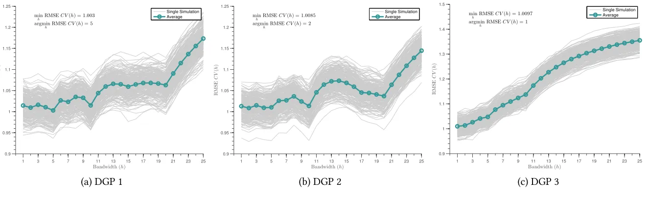
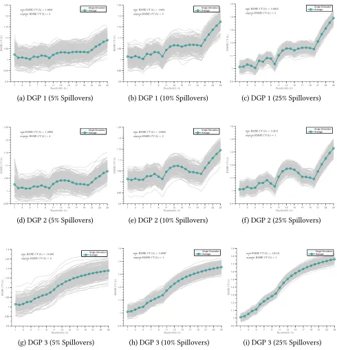
In Figure 1, we consider the cross validation search forh∗ in each model following the LOOCV procedure described in section3.2. These figures correspond to cases where the stochastic error term follows a normal distribution with mean zero and standard deviation of 1, and where spillovers occur to 10% of the total sample. Full sets of figures corresponding to spillovers reaching a smaller and larger
portion of the sample are provided in Appendix Figure A1. These figures plot the Root Mean Squared Error associated with a range of potential search bins for spillovers,h, where in each case, a givenhwill then result in inclusion of “close to treatment” indicators up until the marginal close to treatment unit results in insignificant estimates. According to the procedure described above, the optimal spillover binh∗to use in the spillover-robust DD procedure is that which minimises RMSE among all competing options.
Figure1displays the RMSE for each of a range of values ofh varying from 1 to 25 (displayed on thex-axis). We stop searching ath = 25 in this case as RMSE only increases after this point. The left-hand panel displays values associated with model 1, the centre panel displays values associated with model 2, and the right-hand panel describes values for model 3. In each case, thin gray lines represent a single simulation, while the thick green line represents averages over the full set of simulations. We see that overwhelmingly, the RMSE procedure recovers “correct” search bins based on the DGPs
described previously. In model 1, optimal RMSE corresponds to distance of 5, in line with the 5 unit spillover bins, model 2 results in a minima ath = 2, and model 3 (the non-linear specification) results in optimally choosing a short search bandwidth to closest approximate the smooth decrease in spillovers over distance from the exponential function. In Appendix Figure A1similar figures are presented for cases where spillovers reach larger (25%) or smaller (5%) portions of the population. Generally optimally determined bandwidths agree with those discussed here, however in cases where spillovers occur to a
larger proportion of the population, greater power results in a smaller optimal bandwidth for model 2, in which irregular spillovers occur. In the case where spillovers reach 25% of the population (Appendix FigureA1f),h∗is determined as 1, allowing for irregular spillovers to be perfectly captured.
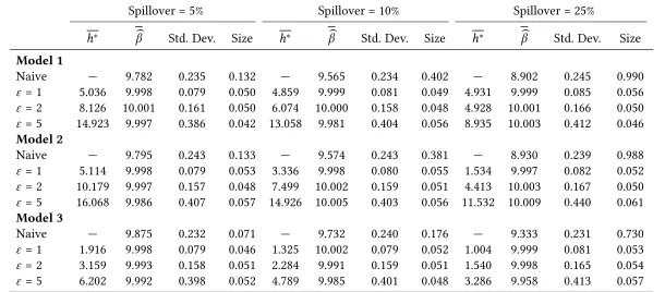
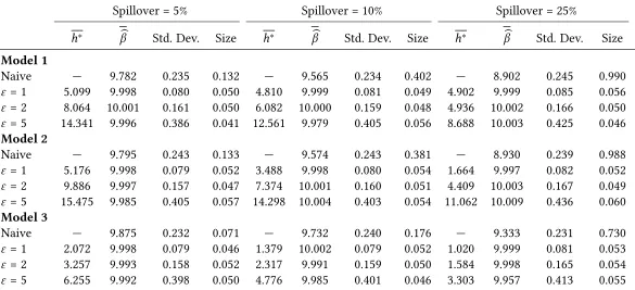
effects themselves. In Table1, I provide estimated treatment effects from the spillover-robust DD mod-els, along with the size of tests when examining the null that β=10, at a 5% significance level. If the spillover-robust DD model correctly recovers parameters in repeated simulations, the size of the test
should be approximately 0.05. Table 1 presents estimates associated with each of the 3 DGPs in separate panels, varying the degree of spillovers in columns, and the noise due to the stochastic error term be-tween rows. In each case, we first present the naive estimate forβ when not considering any spillovers. In each case, we observe that (unsurprisingly) naive models perform very poorly. Given that spillovers are of the same direction as treatment itself, we see that in each case, failing to account for spillovers results in attenuation of estimated treatment effects, as well as considerable over-rejection of the null.
What’s more, naive DD models perform increasingly worse when spillovers propagate to a larger pro-portion of the population. This results is exactly as outlined in the bias calculation documented in equation 16. Moving across columns, the proportion of the control group which is contaminated by spillovers increases, and so the bias increases in magnitude.12
Turning now to models in which spillover-robust DD models are estimated, we see that unlike the naive models, parameter estimates as well as the size of hypothesis tests perform correctly. For each
model simulated, and for each value of the stochastic error term and degree of spillovers in Table1, the size of the test is good, and estimated treatment effects are extremely close toβ = 10. In considering the size of tests, rates of rejection of the null are always within±0.008 of the expected rate of 0.05, and indeed are often exactly 0.05 (based on 2,500 simulations). It is important to note that this occurs even when models are mis-specified in the spillover robust-DD search procedure. For model 2 and model 3, determining spillovers with a constanth will generally fail to capture the true DGP, but as we see in
Monte Carlo tests, it does allows us to correctly estimate treatment effect, even when the simulation process is noisy. Similarly, even though at times we observe that average h∗ across simulations are not precisely as in the DGP (especially when more noise is introduced), we observe that the proposed procedure results in good properties in testing.
12Indeed, we can also show that the bias formula holds as derived (subject to minor variation due to variation in
simu-lation). Considering equation16and model 1 with 10% spillovers from Table1, the expectation forβbis:
E[βb] = 10−5 0.025 1−0.2−4
0.025 1−0.2−3
0.025 1−0.2 −2
0.025
1−0.2 = 9.5625
Figure 1: Root Mean Squared Error and Bandwidth Search
1 3 5 7 9 11 13 15 17 19 21 23 25
0.9 0.95 1 1.05 1.1 1.15 1.2 1.25
Bandwidth (h)
R M S E C V ( h ) min h RMSE
C V(h) = 1.003
argmin
h RMSEC V(h) = 5
Single Simulation Average
(a) DGP 1
1 3 5 7 9 11 13 15 17 19 21 23 25 0.9 0.95 1 1.05 1.1 1.15 1.2 1.25
Bandwidth (h)
R M S E C V ( h ) min h RMSE
C V(h) = 1.0085 argmin
h RMSEC V(h) = 2
Single Simulation Average
(b) DGP 2
1 3 5 7 9 11 13 15 17 19 21 23 25
0.9 1 1.1 1.2 1.3 1.4 1.5 Bandwidth (h) R M S E C V ( h ) min h RMSE
C V(h) = 1.0097
argmin
h RMSEC V(h) = 1
Single Simulation Average
(c) DGP 3
Notes to figure1: Root mean squared error (RMSE) under various data generating processes is displayed, allowing for spillovers calculated using bandwidthh. Gray
solid lines present alternative simulations (250 simulations shown here), and the solid green line with circles documents the average RMSE for each bandwidth over the full set of simulations. DGPs are laid out fully in section4.1. For each simulation,N = 1000 observations andε∼ N(0,1). 20% of the sample are treated units, and 10% of the sample are “close to treated” in the original DGPs. Identical plots for alternative degrees of spillovers are displayed in Appendix FigureA1. The RMSE calculated for each bandwidth shown is based on the iterative procedure described in the text, with the optimal spillover-robust DD model corresponding to that estimated using the bandwidth which returns the lowest RMSE. The minimum RMSE and the minimum bandwidth associated with this RMSE (ie the optimal model bandwidth) is displayed in each panel.
Table 1: Monte Carlo Simulation: Optimal Bandwidth and Average Treatment Effects
Spillover = 5% Spillover = 10% Spillover = 25%
h∗ βb Std. Dev. Size h∗ βb Std. Dev. Size h∗ βb Std. Dev. Size
Model 1
Naive — 9.782 0.235 0.132 — 9.565 0.234 0.402 — 8.902 0.245 0.990
ε = 1 5.036 9.998 0.079 0.050 4.859 9.999 0.081 0.049 4.931 9.999 0.085 0.056
ε = 2 8.126 10.001 0.161 0.050 6.074 10.000 0.158 0.048 4.928 10.001 0.166 0.050
ε = 5 14.923 9.997 0.386 0.042 13.058 9.981 0.404 0.056 8.935 10.003 0.412 0.046
Model 2
Naive — 9.795 0.243 0.133 — 9.574 0.243 0.381 — 8.930 0.239 0.988
ε = 1 5.114 9.998 0.079 0.053 3.336 9.998 0.080 0.055 1.534 9.997 0.082 0.052
ε = 2 10.179 9.997 0.157 0.048 7.499 10.002 0.159 0.051 4.413 10.003 0.167 0.050
ε = 5 16.068 9.986 0.407 0.057 14.926 10.005 0.403 0.056 11.532 10.009 0.440 0.061
Model 3
Naive — 9.875 0.232 0.071 — 9.732 0.240 0.176 — 9.333 0.231 0.730
ε = 1 1.916 9.998 0.079 0.046 1.325 10.002 0.079 0.052 1.004 9.999 0.081 0.053
ε = 2 3.159 9.993 0.158 0.051 2.284 9.991 0.159 0.051 1.540 9.998 0.165 0.054
ε = 5 6.202 9.992 0.398 0.052 4.789 9.985 0.401 0.048 3.286 9.958 0.413 0.057
Notes: Models 1, 2 and 3 are described in section4.1. The top line of each panel and model presents naive estimates without correcting for
spillovers, while each line below consists of 2,500 simulations applying the spillover robust estimation technique. h∗ refers to the average
spillover distance calculated in cross-validated models,βbthe average parameter estimate forβ (which is equal to 10 in the true DGP) with its standard deviation among 2,500 trials, and the size reports the proportion of true null hypothesesH0 :β = 10 rejected atα = 0.05 across the
2,500 trials. The optimal bandwidthh∗for spillover-robust DD models are determined using Leave-One-Out Cross-validation.
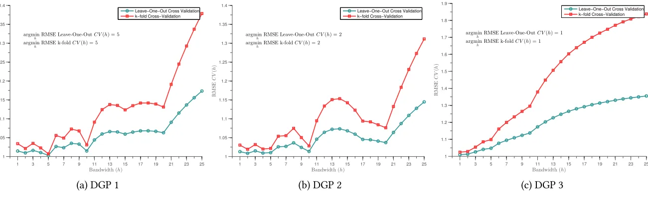
Finally, it is important to note that while RMSE calculated using LOOCV leads to (generally) cor-rectly captured spillover bandwidths, and estimated treatment effects with good size properties, in certain cases the use of LOOCV will be computationally infeasible, specifically as the number of
ob-servations grows. In these cases,k-fold CV offers a computationally convenient alternative manner to calculateh∗. We document in Appendix FigureA2and Appendix TableA1, that the use ofk-fold CV results in identical optimal spillover bins, even if calculations of the RMSE are generally higher when generated usingk-fold CV, given that predictions are made using fewer training observations. Further-more, when considering the parameters estimated usingk-fold, rather than LOO, CV we find largely similar results in terms of size and estimated parameters. These are fully documented in Appendix
TableA1, where performance is qualitatively identical. We demonstrate a case wherek-fold CV is of considerable use below in an extended empirical example.
4.2
An Applied Example: Test Messaging Bans and Local Spillovers over
Roadways
In order to examine the performance of the spillover-robust DD strategy in an applied setting we
con-sider estimates from an existing DD study, in which only headline treatment are estimated, but in which propagation of treatment over space may plausibly occur. To do this, we revisit the results ofAbouk and Adams(2013), who examine the passage of state-level laws in the US prohibiting the sending of text messages while driving. While Abouk and Adams(2013) document a range of impacts of these laws on rates of deaths in Single Vehicle Single Occupant (SVSO) accidents in a DD setting, they restricted their attention only to the impacts on accidents occurring in the same states in which reforms were
implemented.
Nevertheless, there is reason to suspect that laws of this type will not be uniquely restricted to the states where they are passed. If drivers do actually alter their behaviour in the presence of the law, it is plausible that their behaviour may not immediately revert to be what it would have been in the absence of the law when driving across state boundaries. In particular, there are various outcomes which may be observed. Firstly, it is possible that drivers who are convinced by the state law to reduce
the usage of mobile phones when driving will maintain their improved behaviour when crossing into nearby states, with perceptible reductions in mortality on roadwaysalsoin areas close to the borders of treated states. Alternatively, an unintended behaviour may be observed, where the law simply causes inter-state drivers to hold-off on using their mobile phone when driving until they cross into areas without a law, meaning that any estimates of the reform’s impact using fatal accidents in-state actually overstates the true impact. These two potential behaviours work in opposite directions, suggesting
spillover robust DD models allows for the resolution of an empirically relevant policy and behavioural question.
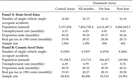
Abouk and Adams(2013) collect data on all text-messaging bans passed into state law between 2007 and 2010, and use data on all fatal accidents over this period from the Fatality Analysis Reporting System (FARS) of the National Highway Traffic Safety Administration. They also classify text-messaging bans into two broad classes: weak or strong, which depends on whether text-messaging is a primary (strong) or secondary offense or restricted to young drivers (weak).13 In the original paper the authors collapse accidents to state by month cells, for 48 months (Jan 2007-Dec 2010) for 49 states (Alaska is removed due to missing data). The original paper estimates DD models focusing on the rate of accidents by state, and
the impact of the different text-messaging bans. In order to examine the occurrence of local spillovers, we consider the impact on a county-by-county basis here. This permits for a much finer analysis of the distance to treatment. In Appendix Table A2we provide the original (state-level) summary statistics of dependent and independent variables fromAbouk and Adams(2013), and below identical variables collected at a county-level. Appendix FigureA3documents the geographic distribution of all accidents along with state and county boundaries. In Appendix TableA3we replicate their full DD analysis at the county-level, finding largely identical results, and in Appendix TableA4we show simple DD models
without yet considering for the presence of spillovers at both the original (state) level in panel A, and
the new (county) level in panel B.
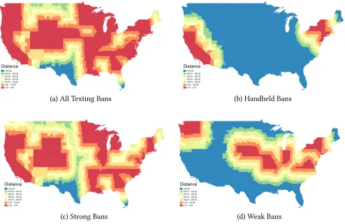
Figure2displays the states which at any point pass different types of text-messaging bans during the period under study, as well as the distance to treatment from each (un-treated) county in the mainland US. These distances refer to the average distance from each county to the nearest treated state border.14
We present treatment status as well as distance to treatment for each of the three types of text messaging bans considered in Abouk and Adams(2013): handheld bans in panel 2b, primarily-enforced bans in panel2c, and secondarily-enforced bans in panel2d, as well as the distance to any type of ban in panel
2a. The original list of states enacting test messaging bans along with the date of enactment, as well as the type of ban enacted can be found in Table 1 ofAbouk and Adams (2013). The distance from each county displayed in Figure 2 is calculated in kilometres, ranging from 0 km (treated) to greater than 500 km. While it seems extremely unlikely that any impact of the bans would propagate even as much as 100 km from a treated state into nearby counties, we show distances up to 500 km to demonstrate that even if spillovers travelled for as much as 500 km, then there would still be additional untreated
13Classification as a primary offense allows for suspected drivers to be pulled over even if no other crime has been
committed, while secondary offenses do not allow this. Further discussion is provided in Abouk and Adams(2013, pp. 183–184).
14In this case, the relevant distance is based on travelling over roads from the nearest treated state, and so closest state
states for each case. This is a fundamental assumption for the spillover-robust DD method, where we require that SUTVA hold between at least some units.
Figure 2:Distances between Counties and Treatment States
>500.00 400.00 − 500.00 300.00 − 400.00 200.00 − 300.00 100.00 − 200.00 0.00 − 100.00 0.00 − 0.00
Distance
(a) All Texting Bans
>500.00 400.00 − 500.00 300.00 − 400.00 200.00 − 300.00 100.00 − 200.00 0.00 − 100.00 0.00 − 0.00
Distance
(b) Handheld Bans
>500.00 400.00 − 500.00 300.00 − 400.00 200.00 − 300.00 100.00 − 200.00 0.00 − 100.00 0.00 − 0.00 Distance
(c) Strong Bans
>500.00 400.00 − 500.00 300.00 − 400.00 200.00 − 300.00 100.00 − 200.00 0.00 − 100.00 0.00 − 0.00 Distance
(d) Weak Bans
Notes to figure2: Each panel displays distances of each county to the nearest treatment state once all bans have been
enacted. States indicated in red are those treated in each case. Panel (a) displays distances to any types of bans, panel (b) displays cases with a universal concurrent hand-held ban, panel (c) displays only bans with primary enforcement, and panel (d) displays bans only with secondary enforcement. Distances are displayed by county, based on the distance from the centre of each county to the closest point on the border of the closest treated state.
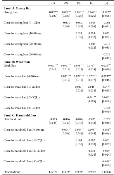
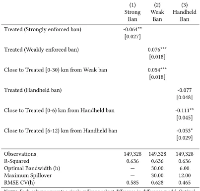
We extend the results ofAbouk and Adams (2013) to consider spillovers, in each case following precisely their variable measurement, controls, estimation sample, and probability weights, however at the county level, rather than the state level. Thus, the baseline DD specification for each type of ban is, following their equation 1:
Yim =α +γi+δm +Ximβ+ωBim+εim (22)
whereYimrefers to the log number of accidents + 1 for countyiand monthm,γ a series of county fixed
effects (for the 3,111 counties of the 49 states used in the original analysis), andδmfixed effects for the 48
months of data. County by month cells are weighted by county population, and additional controlsXim