Energy efficiency programs in the context of increasing block tariffs: The case of residential electricity in Mexico

(1)

Munich Personal RePEc Archive

Energy efficiency programs in the

context of increasing block tariffs: The

case of residential electricity in Mexico

Hancevic, Pedro and Lopez-Aguilar, Javier

Centro de Investigacion y Docencia Economicas

July 2017

(2)

Energy efficiency programs in the context of

increasing block tariffs: The case of residential

electricity in Mexico

Pedro Ignacio Hancevic

∗

Javier Alejandro Lopez-Aguilar

†

June 30, 2017

Abstract

Increasing block pricing schemes represent difficulties for applied researchers who try to recover demand parameters, in particular, price and income elasticities. The Mexican residential electricity tariff structure is amongst the most intricate around the globe. In this paper, we estimate the residential electricity demand and use the corresponding structural parameter estimates to simulate an energy efficiency improvement scenario, as suggested by the Energy Transition Law of December 2015. The simulated program consists of a massive replacement of electric appliances (air conditioners, fans, refrigerators, washing machines, and light-bulbs) for more energy-efficient units. The main empirical findings are the following: overall residential electricity consumption decreases 8.9% and the asso-ciated expenditure falls 11.1%. Additionally, the electricity subsidy decreases 360 million of USD per year and there is an annual cut in CO2emissions of 3.5 million of tons.

Keywords: increasing block pricing, energy efficiency, residential electricity users, elec-tric appliances, energy subsidies, air pollution

JEL classification:D12, L50, L94, Q40, Q53

∗_{Centro de Investigaci´on y Docencia Econ´omicas, Mexico. E-mail:}_{[email protected]}

†_{Centro de Investigaci´on y Docencia Econ´omicas, Mexico. E-mail:}_{[email protected]}

(3)

The Energy Transition Law was enacted in December 2015 (ETL-2015). It mandates the

Mexican Ministry of Energy to undertake technical analysis to evaluate the potential effects

that various energy efficiency measures would have on: (1) electricity subsidy reduction, (2)

household welfare (due to the expected lower electricity bills), and (3) the environment –i.e.,

air pollution and water resources.1 Although some hesitant, non-conclusive, engineering based

reports have been written, there is no economic study that evaluates the potential performance

of the proposed energy efficiency measures.

A very reduced number of papers study energy efficiency in Mexican households (Davis

et al., 2014; Guti´errez-Mendieta, 2016; J. Rosas-Flores, D. Rosas-Flores and D.

Morill´on-G´alvez,2011). In particular,Davis et al. (2014) put under scrutiny and evaluate a large-scale

appliance replacement program in Mexico during the 2009–2012 period.2 Our paper goes

beyond that historical point, and analyzes a set of potential future policy scenarios, which

are expected to happen once the prospective regulations derived from the ETL-2015 become

effective.

With the above objective in mind, we first specify and estimate a structural electricity

de-mand model for residential users in Mexico. We use the corresponding estimates of price and

income elasticities and the coefficients associated to electric appliances as well as other relevant

variables in the demand function, to simulate different energy efficiency scenarios (programs)

that go in line with the ETL-2015 requirements. Concretely, we follow the report by the

Mex-ican Energy Ministry (SENER, 2017b) to assume realistic improved energy efficiency levels

for a selected group of sensible electric appliances: air conditioners, fans, refrigerators,

wash-1_{The ETL-2015 also requires the conduction of research to evaluate the potential impact of distributed}

photo-voltaic generation on the same objective variables –i.e., electricity subsidy, household welfare, and pollution reduction. SeeHancevic et al.(2017) for a complete analysis on this topic.

2_{Davis et al.}₍₂₀₁₄_{) find evidence that refrigerator replacement reduce electricity consumption by 8 percent}

(4)

ing machines, and light-bulbs. We then estimate the counterfactual electricity consumption

levels, assuming each household re-optimizes its choice after the simulated energy efficiency

measures are applied. Finally, using the results of the empirical exercise just described, we

calculate the effects that improved energy efficiency would have on government savings and

air pollution.

The residential electricity tariff structure in Mexico is very intricate.3 There are seven

differenttariff classesacross the country and eigth tariff regions, which are linked to average

temperatures in a subsidized scheme –i.e. high temperature zones afford lower marginal prices

and have larger consumption blocks. Each tariff class consists of increasing block prices (IBP),

which clearly invalidate any simple estimation strategy that relies on OLS or even traditional

IV methods. In the presence of IBP, consumers face a piecewise-linear budget constraint.

These pricing schemes present a serious simultaneity problem: prices and quantities consumed

are endogenously and simultaneously determined (see, for example,Reiss and White (2005),

Olmstead et al.(2007), or Olmstead (2009)). When the joint decision of marginal price and

quantity is ignored in the demand estimation, price effects are likely to be positively biased.4

Our structural model solves this endogeneity problem and allows us to identify the behavior

of residential users. By the same token, we are able to simulate counterfactual scenarios for

relevant energy efficiency programs.

The main results of this study are the following: on average, the residential electricity

con-sumption and the associated expenditure fall 8.9% and 11.1%, respectively. There is, however,

significant heterogeneity with regards of the final effect across households. The reasons are

threefold: the tariff structure differs across the country (i.e., distinct marginal prices and

differ-ent consumption blocks), the electric appliances under study have uneven penetration levels,

and their potential savings are dissimilar. AC units and refrigerators offer the best

opportuni-3_{Mexico has one of the most complex tariff and subsidy structures in the world, see for example}_{Komives et al.}

(2009) andLopez-Calva and Rosell´on(2002).

(5)

ties in terms of policy outcomes: they provide the largest consumption savings, 13% and 5%,

respectively. Finally, the electricity subsidy burden is reduced in about 360 million USD/year,

and there is an annual cut in CO2emissions of approximately 3.5 million of metric tons.

The rest of this paper is organized as follows. Section 1 develops the structural demand

model to be estimated later. Section2illustrates the Mexican residential electricity sector and

presents a description of the data used in the empirical analysis. Section3 presents the

esti-mation results. Section4describes the counterfactual scenario and then presents the estimated

impact that improved energy efficiency would have on household electricity consumption, the

residential electricity subsidy, and the environment. Finally, section5concludes the paper.

1

Structural model

In this section we present the structural model of electricity demand. The key feature of the

model is the underlying piecewise linear budget constraint that emerges in the context of IBP.

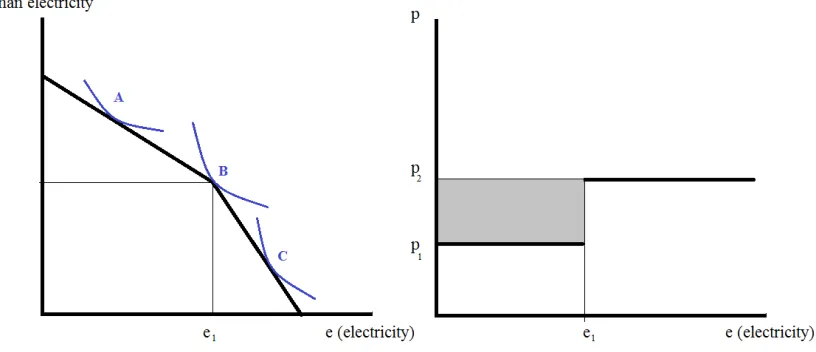
Figure1illustrates this point for a two-block tariff scheme. A consumer can choose a quantity

of electricity in the first block (point A in the left panel of Figure1), where the marginal price

is p1 (right panel). Another possibility is the consumer chooses a quantity in the second

con-sumption block (point C in the left panel) and pays a higher marginal price p2(right panel). A

third possibility is that the consumer choosese1, which is exactly the kink point. The

underly-ing idea is that consumers behaveas if they where making a discrete–continuous choice. They

first select the consumption block, and then, conditional on being in the the selected block,

they choose the quantity of electricity. A maintained assumption in our paper is therefore that

consumers respond to marginal prices.

FIGURE1ABOUT HERE

(6)

behave rationally and respond to marginal prices in the context of IBP schemes. In particular,

Borenstein (2009) suggests consumers respond to expected marginal prices, and Ito (2014)

finds evidence that consumers respond to average prices rather than marginal or expected

marginal prices. Both studies use billing panel data for a relatively small geographical area

in Southern California. Although we acknowledge their findings, especially the clean

em-pirical strategy followed by Ito (2014), we are unable to apply his methodology due to data

limitations and cannot formally test the implicit rationality assumption made in our structural

model of consumer choice. On the other hand, Nataraj and Hanemann(2011) find evidence

that water consumers who face IBP do respond to changes in marginal prices. The

discrep-ancy between the results obtained for water and electricity consumption could be, in principle,

due to fundamental differences between the two services (water and electricity cover and

sat-isfy different needs) and/or differences between the price structures under investigation. In any

case, and not just as a simple justification, the above-mentioned piece of evidence for a reduced

area in Southern California (Borenstein,2009;Ito,2014) cannot be directly extrapolated to all

settings and countries. Also, given the data limitations we face, the empirical strategy followed

in this study is still superior than common approaches that use average prices in the context of

OLS regressions or IV specifications (usually based on weak instruments), which ignore the

multi-block structure.

As pointed out in Olmstead (2009), there are two main advantages of structural models

of the sort described above over the traditional reduced-form approaches –either OLS or IV

models. First, structural models (potentially) produce unbiased and consistent estimates of

parameters such as price and income elasticities. Second, they are consistent with a

utility-maximizing behavior and allow the researcher to perform meaningful counterfactual analysis,

such as measurement of welfare changes due to price adjustments or other policy changes.

The structural discrete/continuous choice (DCC) model was originally proposed by

(7)

income taxation. In the more specific context of consumer choice, the model was developed

by Hanemann (1984). The typical electricity demand function estimated in most empirical

applications has the following log-log form:

lnejt =α lnpjt+γ lnyjt+Xjt β+vjt (1)

where ejt is the quantity of electricity consumed by the household j in period t, pjt is the

marginal (or sometimes, the average) price of electricity, yjt is the household income, and

Xjt is a vector of variables that includes household characteristics, dwelling characteristics,

weather variables, and several other control variables. Our model closely follows the model

proposed by Hewitt and Hanemann (1995) for water demand, later extended by Olmstead

et al. (2007). It incorporates a compounded error term vjt =ωj+εjt. The first part of the

error, ωj, includes unobserved (to the econometrician) household preferences for electricity

consumption, whereas εjt includes both optimization errors and the traditional measurement

error. We assume thatωj∼N(0,σ2ω)and thatεjt ∼N(0,σ2ε). We also assume that both error

terms are independently distributed. Hence, the compounded errorvjt ∼N 0,σ2ω+σ2ε

.

In the environment of IBP, one must distinguish between conditional and unconditional

demand functions. The former is defined as the quantity the household consumes conditional

on being in themth price block. This is reflected in equation (1) evaluated at the price pmand

thevirtual incomeyˆm=y+δm, whereδm=0 ifm=1, andδm=∑m_i₌−₁1(pi+1−pi)eiifm>1.

The termeirefers to the the upper limit of the block (kink point)i. 5

Each household has separate conditional demand functions, one for each block. On the

other hand, there is only one unconditional demand function that characterizes the overall

con-sumption choice. Omitting household and time subscripts, defineeas the observed

consump-5_{Notice that the shaded area in Figure}₁_represents_δ

mevaluated atm=2. This term constitutes the implicit

(8)

tion, e∗_mas the optimal consumption on blockm, andemas the consumption at the kink point

m. We estimate the unconditional demand function using a Maximum Likelihood approach.

The log-likelihood function is as follows

lnL=

∑

ln

      M

∑

m=1

"

1

p

2πσ2

v

∗exp −(lne−lne

∗

m)

2

2σ2

v

!#

∗Pr(blockm)

+ M−1

∑

m=1

"

1

p

2πσ2_ε ∗exp

−(lne−lnem)2

2σ2_ε

!#

∗Pr(kinkm)       (2) where

Pr(blockm) =Φ

lnem−lne∗m σω −ρ

lne−lne∗ m σv

p

1−ρ2

!

−Φ

lnem−1−lne∗m σω −ρ

lne−lne∗ m σv

p

1−ρ2

!

and

Pr(kinkm) =Φ

_ln

em−lne∗_m₊₁

σω

−Φ

lnem−lne∗m

σω

Φ(.) is the normal CDF and ρ=corr(v,ω). Notice that each observation in the likelihood

function has positive probability of having occurred in any segment and any kink point of the

budget constraint. We use the estimated parameters to calculate the expected unconditional

demand, as well as price and income elasticities.

2

Data and context

Our main source of data is the National Survey of Household Income and Expenditure (ENIGH),

which is collected every two years by the National Institute of Statistics and Geography

(IN-EGI). Specifically, we make use of the surveys 2010, 2012 and 2014. The data collected in

these surveys provide us with certain household and dwelling characteristics –including some

information on the stock of electric appliances–, as well as monthly household expenditures.

(9)

Table1we provide the summary statistics for the relevant variables used in this research.

TABLE1ABOUT HERE

Aside socio-demographic and economic characteristics at the household level, the ENIGH

data include each household electricity expenditure which corresponds to a single billing

pe-riod. This fact allows us to avoid the problems resulting from aggregating consumption data

across billing periods, typically an entire year (see Dubin and McFadden (1984) and Reiss

and White(2005)). Based on household geographic location, we match each household in the

ENIGH with the actual electric rate schedule the household faces. For that purpose, we use

tar-iff data provided by the national electricity company that is in charge of electricity distribution

all across the country (Comisi´on Federal de Electricidad, CFE). We therefore invert the

corre-sponding tariff formula and retrieve the electricity consumption (in kWh) from the electricity

expenditure data provided in the ENIGH.

There are seven different tariff classes (i.e., categories): 1, 1A, 1B, 1C, 1D, 1E and 1F,

which are set by the CFE based on average temperature during summer months at the

munici-pality level. Each tariff class consists of three or four consumption blocks. The corresponding

block lengths and marginal prices differ considerably across tariff classes for both summer

and winter seasons. We use the month of payment reported by household to classify users

between summer and winter tariff structures.6 Another source of price heterogeneity comes

from the fact that we use three different cross sections: 2010, 2012, and 2014, and the CFE

adjusted block marginal prices in each of those years. Table2provides an example for the rate

schedules during Summer 2014.

TABLE2ABOUT HERE

6_{Billing data reported in the ENIGH correspond to the preceding two months. November to January are the}

(10)

In addition, each of the seven IBP tariff classes has an associated annual maximum

con-sumption threshold. When the threshold is crossed, the corresponding household is

automati-cally classified as a High-Consumption User (DAC). Analogously, when the sum of

consump-tion in the last 12 months falls below the threshold, a DAC user returns to its original tariff

class. The DAC users afford a two-part tariff that is composed of a fixed charge and a uniform

marginal price, which is applicable to any consumption level and substantially more expensive

than the regular IBP tariffs mentioned before. The consumption limit to become a DAC user

differs across tariff classes and the associated marginal price differs over CFE tariff regions.

Since the ENIGH data do not identify the exact tariff class each household belongs to, we need

to make some additional assumptions in order to establish which households are considered

as DAC users in our sample.7 Concretely, we retrieve monthly consumption for each

house-hold using the corresponding DAC tariff structure and then compare it to an imputed monthly

consumption limit (based on the actual annual limit). All households exceeding this limit are

considered to afford a DAC tariff and consequently, for these households we use this retrieved

consumption instead of the one computed based on the original tariff.

The three cross sections used in this paper add up to 52,580 household observations. Our

final sample comprises 41,779 observations. First, we discarded households that either were

not connected to the electricity grid (3,661) or did not have electricity meter (1,468). Second,

we dropped 2,359 households for which it was impossible to identify their actual one-period

electric bill.8 For other 3,166 cases, it was troublesome to retrieve electricity consumption

because they reported to have non-standard billing periods, paid their last bill long time ago or

reported an expenditure in electricity bellow the minimum possible outlay charged by CFE.9

7_{Recall we recover electricity consumption from expenditure data.}

8_{This problem typically emerges in the case of multiple-family households. In those cases, it is not clear}

whether each family reports the share of the bill they actually pay or the total bill amount. Additionally, some households report paying electric bills for more than one family, or even they report paying more than one bill (several months at once).

9_{Our final sample comprises only those observations that reported to pay electricity on a bimonthly basis, and}

(11)

Finally, we dropped 147 observations due to missing values in other sensible variables used in

our estimations. Table3shows the final distribution of users and the average consumption by

tariff classes, comparing the estimated values from the ENIGH data with the the corresponding

figures from the CFE official report for the year 2015. The two set of numbers do not differ

substantially, validating our empirical exercise presented later in this paper.

TABLE3ABOUT HERE

3

Electricity demand estimation

As described in section 2, our database provide us with detailed household-level electricity

demand data. We exploit the substantial cross-sectional and time-series variation in prices that

residential users face in order to estimate the structural DCC model of Equation (2). As a

pure academic concern, we have to mention that the price schedule itself could be endogenous:

the schedule changes over time and varies across tariff classes. While these price variation is

very useful for identifying the price coefficient, using the structural model does not solve the

potential endogeneity issue per se. The schedule changes could be correlated with unobserved

demand shocks not captured in our model. There is however a clear fact in the case of Mexico

that supports our exogeneity assumption: in a context of highly subsidized electricity prices,

authorities design tariff schedules from a (partial) cost recovery perspective –i.e., a supply

side decision. Additionally, the inclusion of state fixed effects and year fixed effects helps

mitigate this (unlikely) endogeneity issue since they reduce, to some extent, the unobserved

heterogeneity.

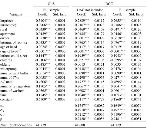
Table4presents the electricity demand models estimates. The first column corresponds to

the simple OLS specification, where the price variable represents the marginal price paid by

(12)

that there is a substantial simultaneity (endogeneity) problem, as it was previously explained.

We present two specifications for the DCC model. One excludes the DAC users and the other

makes use of the full sample. As can be seen, the estimates are relatively similar in both DDC

model specifications, validating the exercise we performed to retrieve consumption of DAC

users (see section2). As a result, we will concentrate in the DDC full sample model for the

rest of the paper, which is our baseline specification.

TABLE4ABOUT HERE

Clearly, in the baseline specification all the estimated coefficients are statistically

signifi-cant and have the expected sign, with the only exception being the dummy variable elderly,

which is not significant at any conventional level. The variables that represent electric

appli-ance holdings (i.e., water-pump, AC unit, fans, number of light bulbs, TV sets, refrigerators,

and washers) have a positive impact on household electricity consumption. In particular,

re-frigerators and AC units have sizable effects.

Table5presents the simulated unconditional price and income elasticities for the two DCC

models described before. We depart from Olmstead et al.(2007) and calculate demand

elas-ticities in the following manner: we first simulate an 1% increment in all marginal prices and

re-calculate household virtual income, ˆym, at each block in order to compute a new predicted

consumption. We then compare the counterfactual predicted consumption with the original

predicted consumption. The bootstrapped average difference across households is the reported

price elasticity. We perform a similar routine to calculate the unconditional simulated income

elasticity. This way, in the baseline model the estimated unconditional elasticities are

approxi-mately -.23 and .19 for price and income, respectively.10

10_{Other short-run estimates of price elasticities in the Mexican residential sector are -0.14 for the State of}

(13)

TABLE5ABOUT HERE

4

Simulated energy efficiency scenario

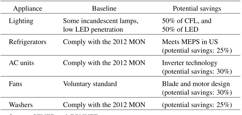
In this section we simulate a massive energy efficiency program that is in line with the Energy

Transition Law of December 2015. For that purpose, we select a group of energy-intensive

appliances that are present in a significant number of Mexican households. Following the report

by SENER (2017b), for each appliance we assumepotential savingsin electricity consumption

by comparing known values from the Mexican Official Norms of Energy Efficiency (MON) –or

estimated baselines– with minimum values of energy consumption from international standards

or new technologies. In a majority of cases, the most efficient equipment is already available in

Mexico, although sometimes at a higher cost and with a substantially lower market penetration

than the equipment considered at the baseline. Table 6presents the assumptions of improved

energy consumption for the set of selected electric appliances.

TABLE6ABOUT HERE

For the simulations, we only use the ENIGH 2014 and take advantage of two facts. First,

this cross section distinguish between incandescent (inefficient) and low-consumption lamps

held by the households. Second, data from ENIGH 2014 are more comparable to the 2015

CFE numbers we use to calculate savings in the electricity subsidy and air pollution emissions.

The simulation exercise consists of the following steps:

1. Compute the predicted electricity consumption for each household using the conditional

demand coefficients of the DCC full-sample model (Table4)

(14)

2. Recover the compounded error term, ˜vjt, as the difference between the observed

con-sumption and the predicted concon-sumption from step 1

3. For each electric appliance considered separately (except for light-bulbs), modify the

corresponding demand coefficient by imputing the associated energy efficiency factor

(Table6) and then obtain the new predicted consumption

4. Add the estimated error term from step 2 to the new predicted consumption of step 3

5. Compare the original (observed) consumption with the predicted consumption of step 4.

It is worth noting that the predicted consumption derived from the DCC baseline model

(step 1 above) is, in fact, the expected unconditional consumption. As a result, the calculation

of the predicted consumption involves a process of re-estimating the probabilities associated to

each consumption block and each kink point, and that is the case for each household regardless

of the original (observed) consumption level.

In the case of light-bulbs, we simulate a massive adoption scenario of compact fluorescent

lamps (CFL). We assume households replace the incandescent lights with CFL up to the point

of reaching at least 50% CFL penetration, as well as an improvement in energy consumption of

75% of CFL with respect to the old incandescent lamps.11 We then compute the counterfactual

consumption.

There is a number of implicit assumptions (limitations) in the simulation exercise of this

section. First, we do not allow for changes in appliance penetration rates. Hence, all

improve-ments in technology has no effect on adoption.12 Second, we consider the energy efficiency

im-provement in a given appliance affects uniformly all households holding the appliance. Third,

11_{For instance, this is equivalent to assuming a household replace a 60-watt incandescent lamp with a new}

15-watt CFL.

12_{More specific data on the characteristics of household electric appliances would make possible to estimate}

(15)

since we do not have information on the brand and model of electric appliance held by the

household, we do not know the ex-ante unit energy consumption (UEC). As a result, the

im-puted energy efficiency improvement factors are simply averaged measures based on technical

reports from CONUEE and SENER.13 In that sense, having detailed data on household

appli-ance holding would substantially improve the quality of this research. Unfortunately, we do

not have such information.14 Nevertheless, our simulation exercise represents a valuable effort

to measure the potential impacts of the ETL-2015.

4.1

Impact on household consumption and expenditure

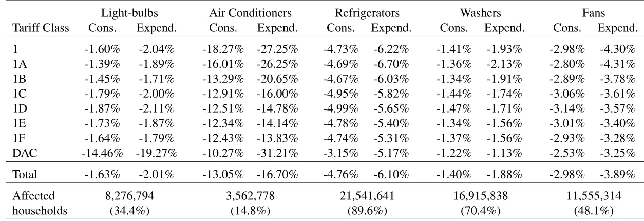
Table 7 presents the impact of the simulated energy efficiency scenario for each appliance

individually considered –i.e., assuming energy efficiency is improved for one appliance at a

time. The table shows the average savings per month in terms of electricity consumption and

expenditure for affected households only –i.e., households that have at least one unit of the

appliance under analysis.15 AC units has the lowest penetration rate (14.8%) but the highest

impact on electricity consumption and expenditure (13% and 16.7% savings, respectively).

Refrigerators, in turn, have the largest penetration rate (89.6%) and the second highest savings

(4.8% and 6.1%).

TABLE7ABOUT HERE

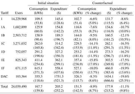
Table 8displays the average savings in terms of consumption and expenditure when

im-provements in energy efficiency occur in all selected appliances simultaneously. In this case,

the results are computed considering the full 2014 sample. In that context, the final impact

13_See_SENER₍_2017b_),_{LBNL and IIE}₍_2011a_{) and}_{LBNL and IIE}₍_2011b₎

14_{A great deal of relevant literature on residential energy efficiency is about interventions through frame field}

experiments. See for exampleGandhi et al.(2016) orHahn and Metcalfe(2016) for a review on this topic. We recognize the advantages of such an approach, however field experiments are beyond the scope of this research and the comparisons are, to some extent, meaningless given the totally different contexts.

15_{Recall that we do not consider alternative adoption scenarios, that is to say the current level of appliance}

(16)

on each household savings will depend on the corresponding stock of appliances. The overall

average consumption savings amount to 16.6 kWh per month, which in monetary terms

repre-sents a reduction of $27.3 in the electricity bill. As can be seen, the savings differ substantially

among the different tariff classes, being 1F users the most benefited. At the other end of the

spectrum, tariff 1 users have, on average, the lowest savings.

TABLE8ABOUT HERE

Notice that savings in expenditure are systematically larger than savings in consumption,

as shown in Tables7and8. In fact, that is a direct consequence of the re-estimation of

proba-bilities associated to different consumption blocks.16 Once the improvements in efficiency take

place, in a significant number of cases households not only consume less but also consume in

a lower block –i.e., they pay a lower marginal price. Table9presents the percentage of

house-holds switching to a lower block once improvements in efficiency occur. It also shows the

cases where DAC users reduce consumption sufficiently to return to the original tariff class.

This constitute a significant advantage of our structural model, which provide us with more

flexibility (and realism).

TABLE9ABOUT HERE

4.2

Impact on government savings

The federal government collects the value-added tax (VAT) which has a 16% rate on electricity

sales. Additionally, most local governments collect a street lighting tax with rates ranging from

5% to 10%. However, the government fiscal outcome derived from the residential electricity

sector operation is a large deficit. Household electricity consumption is heavily subsidized:

16_{That is a necessary step to recover the expected unconditional consumption levels, a point previously}

(17)

more than 98% of households receive the electricity subsidy and pay, on average, only 45%

of the overall electricity cost. As a result, the fiscal burden associated to residential electricity

consumption has consistently increased during the last decade and currently represents more

than 0.5% of the Mexican GDP.

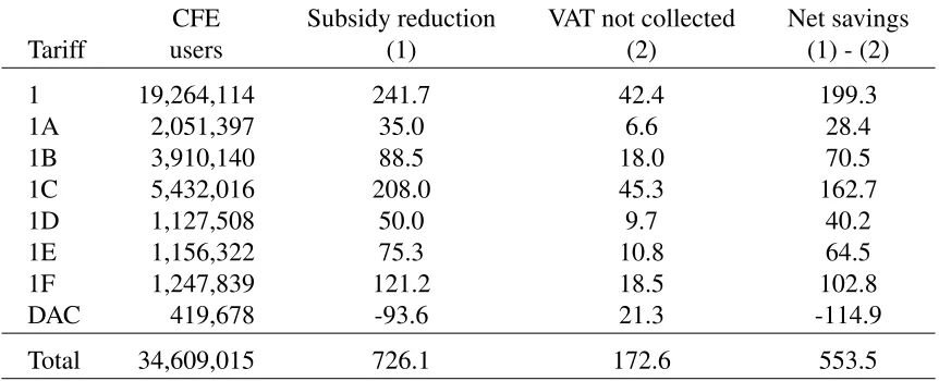
Table 10 displays the effect that the main energy efficiency scenario (i.e., improvements

in energy efficiency occur in all selected appliances simultaneously) would have on federal

government savings. We assume that local governments continue affording the street lighting

costs. The results in the table are calibrated using the actual number of users in each tariff

class according to the CFE official report for the year 2015. The total monthly reduction in the

net subsidy account amounts to 553.5 million of Mexican Pesos (MXP). Although electricity

consumption differs during summer and winter months, a simple (arbitrary and imperfect)

extrapolation of this result would imply annual savings of approximately 6.6 billion of MXP

–i.e., 360 million of USD at the current exchange rate.

TABLE10ABOUT HERE

By decomposing the fiscal outcome into the distinct tariff classes, it is apparent that the bulk

of savings come from the more numerous classes (1 and 1C). On the other hand, the changes

in both consumption and composition of DAC users have a negative impact on the subsidy

account. The reason is simple: DAC users pay for electricity approximately 50% above the

real supply cost, and therefore cross-subsidize users in other tariff classes.

4.3

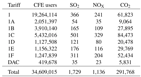
Impact on air pollution

Electricity generation in Mexico is heavily based on fossil fuels (approximately 80% of the

(18)

accounts for 25% of total electricity consumed in the country.17 In this section we calculate

the environmental impact of the simulated energy efficiency scenario. Our analysis relies on

the emission factors recently published by SENER(2017a), which were calculated assuming

the typical operation of an average thermal generator.18 Table 11 presents the environmental

outcomes of the massive energy efficiency scenario.

TABLE11ABOUT HERE

The technologies used for electricity generation are: coal, combined cycle, internal

com-bustion, turbo-gas and conventional steam (fuel-oil and gas). It is important to note that, since

2015, the higher availability of natural gas made it possible to reduce the consumption of more

expensive and polluting fuels, such as fuel-oil and diesel. Hence, the avoided emissions of

local pollutants such as SO2 and NOX are important but not extremely significant since the

country relies more on natural gas, which in this case could be considered a “cleaner” fuel.

With regards of carbon dioxide emissions, it is interesting to put these numbers in context. In

so doing, we transform the results obtained for summer months (shown in table11) to annual

values.19 The estimated annual cut in CO2 emissions is approximately 3.5 million of metric

tons. That figure represents 2.7% of the 2020-2030 emission reduction target for the electricity

generation sector that was committed after COP-21 held in Paris (December 2015).

To provide a monetary metric, we make an additional effort and measure emission savings.

Unfortunately, a market for emissions in Mexico does not exist. There is not a single price for

each of these air pollutants, and no global agreement has been reached. In the case of Mexico,

however, the government sets a tax of approximately 3 USD per ton of carbon emitted. In some

developed countries such as Sweden, the corresponding price could be as high as 130 USD per

17_{Mexico is the 13th largest GHG emitter in the world and the second in Latin America –behind Brazil. It}

contributes with 1.4% of the global GHG emissions (Damassa et al.,2015).

18_{Concretely, the emission factors used in our analysis are: 0.00283 kg/kWh for SO}

2, 0.00186 kg/kWh for

NOX, and 0.47753 kg/kWh for CO2.

19_{Here the same disclaimers of section}_4.2_{apply: this is an imperfect and, to some extent, arbitrary exercise.}

(19)

ton (Ward et al., 2015). Here we assume an intermediate value of 60 MXP/ton. As a result,

the environmental savings due to CO2emissions reduction amounts to 210 million of MXP per

year.

5

Conclusion

In this paper we propose and estimate a structural model of residential electricity demand to

simulate the effects that a massive energy efficiency program in Mexico would have on

house-hold consumption and expenditure, government subsidies, and air pollution. The

character-istics of the tariff structure all across the country make it difficult to rely on simple reduced

form models. In that sense, our structural model, which builds on the model proposed by

Olm-stead et al.(2007) for water demand, allows us to recover sensible parameters of the electricity

demand function to simulate a meaningful counterfactual energy efficiency scenario. The

sim-ulated situation consists of massive replacements of electric appliances in Mexican households

(AC units, refrigerators, fans, washing machines, and lights). It is based on the suggestions of

a previous report bySENER(2017b), which follows the requirements of the Energy Transition

Law of December 2015.

The main results of this study are the following: residential electricity consumption falls

8.9% and the associated expenditure decreases 11.1%, on average. The outcomes, however,

vary significantly across consumers because the tariff structure differs substantially depending

on the geographical location of households. There are different marginal prices and different

consumption blocks at the municipality level, which are linked to the average summer

tem-peratures. Also, the electric appliances under study have very uneven penetration levels and

different potential savings. As a result, electricity consumption and expenditure once the

en-ergy efficiency improvements take place have a variety of responses. Users under 1F tariff are

(20)

tariff class (1) save 8.6% in their electricity bill. In terms of electric appliances, AC units and

refrigerators are probably the best candidates for future policy targets: they proportion, on

aver-age, consumption savings of approximately 13% and 5% on affected users, respectively. With

regards of the residential electricity subsidy, the fiscal burden could be reduced in 360 million

USD per year. Finally, there would be an annual cut in CO2 emissions of approximately 3.5

million of tons, which represents about 2.7% of the 2020-2030 emissions reduction goal for

the electricity generation sector as it was committed in the COP-21 held in Paris.

There are some limitations in our simulation exercise that provide incentives for further

research on this topic. The consumer decisions regarding the replacement of old appliances

and/or the adoption of new technologies were not considered in our model –we assume all

households holding the selected appliance simply replace it for a more efficient unit. Also,

more flexibility in terms of consumer behavior would be welcome: our empirical exercise

as-sumes a uniform effect for all households holding the appliances under consideration.20

There-fore, all the heterogeneity we obtain in our results comes from the differential tariff structure,

the household stock of appliances, and the imputed energy efficiency improvement factors for

each appliance. Finally, detailed information on the actual household stock of appliances (e.g.,

price, operation and maintenance costs, UEC, etc.) and on conservation practices followed by

users would be a plus.

The above discussion points in the direction of suggesting a concrete piece of advice for

in-terested researchers and policymakers: the collection of more detailed consumers data, which

ideally should be combined with interventions through field experiments to evaluate concrete

measures of energy-efficiency policy. In this line of thoughts, engineering-type studies

consti-tute a first (and necessary) step to evaluate the current situation (of buildings materials,

facil-ities, equipment and appliances) and the potential new technologies that could be introduced.

20_{An assumption difficult to support given the evidence from previous studies. See, for example,}_{Davis et al.}

(21)

Structural economic studies that used observational micro-data are an intermediate step. Our

contribution to the literature, and more specifically, to the Mexican case, clearly belongs to this

second step. The final step is the gold standard in the energy efficiency literature: field

ex-periments. They should be performed to evaluate the complex interactions between economic

agents, information problems, market failures, and behavioral biases. As a result, different

policy options can be properly implemented depending on the specific context.

References

S. Borenstein. To what electricity price do consumers respond? residential demand elasticity

under increasing-block pricing. Unpublished manuscript, 2009.

G. Burtless and J. Hausman. The effect of taxation on labor supply: Evaluating the gary

negative income tax experiment. Journal of Political Economy, 86(6):1103–1130, 1978.

K. Caballero-G¨uendolain and L. Galindo-Paliza. El consumo de energ´ıa en M´exico y sus

efectos en el producto y los precios. Problemas del Desarrollo, 38(148):127–151, 2007.

T. Damassa, T. Fransen, B. Haya, M. Ge, K. Pjeczka, and K. Ross. Interpreting indcs:

Assessing transparency of post-2020 greenhouse gas emissions targets for 8 top-emitting

economies. Technical report, WRI Working Paper, 2015.

L. Davis, A. Fuchs, and P. Gertler. Cash for coolers: Evaluating a large-scale appliance

replace-ment program in Mexico. American Economic Journal: Economic Policy, 6(4):207–38,

November 2014.

J. Dubin and D. McFadden. An econometric analysis of residential electric appliance holdings

(22)

R. Gandhi, C. Knittel, P. Pedro, and C. Wolfram. Running randomized field experiments for

energy efficiency programs: A practitioner’s guide. Economics of Energy & Environmental

Policy, 5(2), 2016.

A. Guti´errez-Mendieta. Determinantes de consumo eficiente de energ´ıa el´ectrica en el sector

residencial en M´exico: un enfoque de regresi´on cuant´ılica. Mimeo, 2016.

R. Hahn and R. Metcalfe. The impact of behavioral science experiments on energy policy.

Economics of Energy & Environmental Policy, 5(2), 2016.

P. Hancevic, H. Nu˜nez, and J. Rosellon. Distributed Photovoltaic Power Generation:

Possi-bilities, Benefits, and Challenges for a Widespread Application in the Mexican Residential

Sector. DIW Berlin Discussion Paper, (1663), 2017.

W. Hanemann. Discrete/continuous models of consumer demand. Econometrica, 52(3):541–

561, 1984.

J. Hausman. Taxes and labor supply. Working Paper 1102, National Bureau of Economic

Research, March 1983.

J. Hewitt and W. Hanemann. A discrete/continuous choice approach to residential water

de-mand under block rate pricing. Land Economics, pages 173–192, 1995.

K. Ito. Do consumers respond to marginal or average price? evidence from nonlinear electricity

pricing. American Economic Review, 104(2):537–63, February 2014.

J. Rosas-Flores, D. Rosas-Flores and D. Morill´on-G´alvez. Saturation, energy consumption,

CO2 emission and energy efficiency from urban and rural households appliances in Mexico.

Energy and Buildings, 43(1):10–18, 2011.

K. Komives, T. Johnson, J. Halpern, J. Aburto, and J. Scott. Residential Electricity Subsidies

(23)

LBNL and IIE. Normas de desempe˜no energ´etico m´ınimo para acondicionadores de aire de

tipo ventana en m´exico. Technical report, CONUEE, July 2011a.

LBNL and IIE. Normas de desempeño energético m´ınimo para refrigeradores en méxico.

Technical report, CONUEE, July 2011b.

L. Lopez-Calva and J. Rosell´on. On the potential distributive impact of electricity reform in

Mexico. 2002.

D. Morales-Ram´ırez, J Luyando-Cuevas, and D. Flores-Curiel. Determinantes del consumo

de energ´ıa el´ectrica residencial de la Zona Metropolitana de Monterrey, Nuevo Le´on, en

m´exico. Universidad & Empresa, 22:79–98, 2012.

S. Nataraj and W. Hanemann. Does marginal price matter? a regression discontinuity approach

to estimating water demand. Journal of Environmental Economics and Management, 61(2):

198–212, 2011.

S. Olmstead. Reduced-form versus structural models of water demand under nonlinear prices.

Journal of Business & Economic Statistics, 27(1):84–94, 2009.

S. Olmstead, W. Hanemann, and R. Stavins. Water demand under alternative price structures.

Journal of Environmental Economics and Management, 54(2):181–198, 2007.

J. Ort´ız-Vel´azquez, G. Bueno, and J Arana-Coronado. An´alisis de la demanda residencial de

electricidad en el Estado de M´exico. Econom´ıa, Sociedad y Territorio, 17(53):199–223,

2017.

D. Rapson. Durable goods and long-run electricity demand: Evidence from air conditioner

purchase behavior. Journal of Environmental Economics and Management, 68(1):141–160,

(24)

P. Reiss and M. White. Household electricity demand, revisited. Review of Economic Studies,

72(3):853–883, 2005.

SENER. Primer an´alisis sobre los beneficios de la generaci´on limpia distribuida y la eficiencia

energ´etica en m´exico. Technical report, Secretaria de Energia, 2017a.

SENER. Primer analisis sobre los beneficios de la generacion limpia distribuida y la eficiencia

energetica en mexico. 2017b.

John Ward, Paul Sammon, Guy Dundas, Grzegorz Peszko, Pauline Maree Kennedy, Sebastian

Wienges, and Nicolai Prytz. Carbon leakage: theory, evidence, and policy design.

part-nership for market readiness technical note; no. 11. Technical report, World Bank Group,

(25)

[image:25.612.111.519.177.353.2]

Figures and Tables

(26)

[image:26.792.88.710.113.422.2]

Table 1:

Variable definitions and summary statistics

Variable Definition Mean Std. Dev. Min Max

Household size Number of household members at home 3.84 1.89 1 21 Children =1 if at least one child living at home 0.48 0.50 0 1 Elderly =1 if at least one person age 65 or older living at home 0.22 0.41 0 1 Age of head Age of the head of household (in years) 49.30 15.37 15 97

Rural =1 if the home is located in a rural area 0.14 0.35 0 1 Apartment =1 if the home is located in an apartment 0.06 0.24 0 1 Owner =1 if the home is owned by any member of household 0.76 0.42 0 1 Number of rooms Number of rooms, excluding kitchen and bathrooms 3.99 1.63 1 21 Number of lights Number of lights of any kind in the home 7.43 5.57 1 130

Number of TVs Number of TV sets in the home 1.58 0.95 0 14

Number of refrigerators Number of refrigerators in the home 0.90 0.35 0 5 Number of washers Number of washing machines in the home 0.71 0.48 0 4 Fans =1 if there is at least one fan in the home 0.49 0.50 0 1 AC unit =1 if there is at least one AC unit in the home 0.14 0.34 0 1 Waterpump =1 if there is at least one waterpump in the home 0.28 0.45 0 1

Income Monthly total income (in MXP) 8,863 9,567 91 258,947

Electricity expenditure Monthly electricity expenditure (in MXP) 219 298 21 12,922 Electricity consumption Monthly electricity consumption (in KWh) 170 161 25 2,775

Source: Own elaboration, based on ENIGH 2010, 2012 and 2014.

Number of observations: 20,604 in year 2010; 6,649 in year 2012; and 14,526 in year 2014.

(27)

[image:27.612.105.531.119.388.2]

Table 2:

Residential tariff schedules for Summer 2014

Tariff 1stblock 2nd block 3rdblock 4th block

1 range (KWh) 0 – 75 76 – 140 ≥141 marginal price ($) 0.719 0.847 2.889

1A range (KWh) 0 – 100 101 – 150 ≥151 marginal price ($) 0.719 0.847 2.889

1B range (KWh) 0 – 125 126 – 225 ≥226 marginal price ($) 0.719 0.847 2.889

1C range (KWh) 0 – 150 151 – 300 301 – 450 ≥451 marginal price ($) 0.719 0.847 1.081 2.889

1D range (KWh) 0 – 175 176 – 400 401 – 600 ≥601 marginal price ($) 0.719 0.847 1.081 2.889

1E range (KWh) 0 – 300 301 – 750 751 – 900 ≥901 marginal price ($) 0.601 0.750 0.978 2.889

1F range (KWh) 0 – 300 301 – 1200 1201 – 2500 ≥2501 marginal price ($) 0.601 0.750 1.823 2.889

(28)

[image:28.612.90.536.139.315.2]

Table 3:

Percentage of users and average monthly consumption by tariff

class: own calculation based on ENIGH data versus CFE users in 2015

ENIGH 2010, 2012, 2014 Official CFE data for 2015a Tariff % of users avg. cons. (KWh) % of users avg. cons. (KWh)

1 56.99 112.14 55.66 88.69

1A 6.73 125.90 5.93 98.48

1B 11.99 160.89 11.30 138.35

1C 14.91 252.29 15.70 228.39

1D 3.35 294.45 3.26 276.74

1E 2.83 414.64 3.34 386.23

1F 2.68 615.04 3.61 663.00

DAC 0.51 439.85 1.21 500.12

Total 100 169.62 100 157.44

Source: Own elaboration based on ENIGH 2010, 2012 and 2014, and CFE tariffs.

(29)

[image:29.612.94.579.118.541.2]

Table 4:

Residential electricity demand model estimates

OLS DCC

Full sample DAC not included Full sample Variable Coeff. Std. Error Coeff. Std. Error Coeff. Std. Error

ln(price) 0.5404∗∗∗ _0.0001 _-0.2889∗∗∗ _0.0117 _-0.2655∗∗∗ _0.0110

ln(income) 0.0906∗∗∗ _0.0001 _0.2167∗∗∗ _0.0073 _0.2186∗∗∗ _0.0075

rural -0.0439∗∗∗ _0.0001 _-0.0469∗∗∗ _0.0108 _-0.0471∗∗∗ _0.0120

apartment -0.0139∗∗∗ _0.0002 _-0.0485∗∗ _0.0179 _-0.0446∗ _0.0203

owner 0.0230∗∗∗ _0.0001 _0.0601∗∗∗ _0.0099 _0.0618∗∗∗ _0.0100

ln(num. of rooms) 0.0335∗∗∗ _0.0002 _0.0765∗∗∗ _0.0114 _0.0767∗∗∗ _0.0119

age of head 0.0074∗∗∗ _0.0000 _0.0117∗∗∗ _0.0017 _0.0119∗∗∗ _0.0017

(age of head)2 -0.0001∗∗∗ _0.0000 _-0.0001∗∗∗ _0.0000 _-0.0001∗∗∗ _0.0000

ln(household size) 0.1147∗∗∗ _0.0001 _0.1959∗∗∗ _0.0097 _0.1942∗∗∗ _0.0092

children -0.0106∗∗∗ _0.0001 _-0.0321∗∗∗ _0.0105 _-0.0295∗∗ _0.0107

elderly 0.0185∗∗∗ _0.0002 _-0.0013 _0.0121 _0.0035 _0.0136

waterpump 0.0044∗∗∗ _0.0001 _0.0438∗∗∗ _0.0099 _0.0478∗∗∗ _0.0104

num. of light bulbs 0.0014∗∗∗ _0.0000 _0.0090∗∗∗ _0.0011 _0.0090∗∗∗ _0.0011

num. of TVs -0.0038∗∗∗ _0.0001 _0.0290∗∗∗ _0.0053 _0.0271∗∗∗ _0.0048

AC unit 0.4306∗∗∗ _0.0002 _0.4727∗∗∗ _0.0145 _0.4695∗∗∗ _0.0144

num. of refrigerators 0.1905∗∗∗ _0.0002 _0.2067∗∗∗ _0.0136 _0.2041∗∗∗ _0.0152

num. of washers 0.0365∗∗∗ _0.0001 _0.0608∗∗∗ _0.0091 _0.0601∗∗∗ _0.0090

fans 0.1245∗∗∗ _0.0001 _0.1040∗∗∗ _0.0092 _0.1053∗∗∗ _0.0101

constant 0.6709∗∗∗ _0.0009 _3.3117∗∗∗ _0.0727 _3.1860∗∗∗ _0.0742

σε 0.1747∗∗∗ 0.0082 0.1649∗∗∗ 0.0079

σω 0.4910∗∗∗ 0.0047 0.4927∗∗∗ 0.0046

σv 0.5212∗∗∗ 0.0036 0.5196∗∗∗ 0.0036

ρ 0.9420∗∗∗ _0.0056 _0.9481∗∗∗ _0.0051

Num. of observations 41,779 41,608 41,779

Notes: ∗∗∗_{significant at}_α₌_0.01. ∗∗_{significant at}_α₌_0.05. ∗∗∗_{significant at}_α₌_{0.10. Dependent}

(30)

[image:30.612.141.491.120.175.2]

Table 5:

Unconditional simulated price and income elasticities

Elasticity DAC not included Full sample

Price -0.2439∗∗∗ _(0.0088) _-0.2263∗∗∗ _(0.0084)

Income 0.1819∗∗∗ _(0.0061) _0.1857∗∗∗ _(0.0063)

Bootstrapped standard errors in parentheses (200 replications).

Table 6:

Energy efficiency assumptions for main electric appliances in the

Mexican residential sector

Appliance Baseline Potential savings

Lighting Some incandescent lamps, 50% of CFL, and low LED penetration 50% of LED

Refrigerators Comply with the 2012 MON Meets MEPS in US (potential savings: 25%)

AC units Comply with the 2012 MON Inverter technology (potential savings: 30%)

Fans Voluntary standard Blade and motor design (potential savings: 30%)

Washers Comply with the 2012 MON (potential savings: 25%)

[image:30.612.113.519.267.460.2]

(31)

[image:31.792.84.711.136.351.2]

Table 7:

Impact of improved energy efficiency by electric appliance:

% change on consumption and expenditure per month (affected households only)

Light-bulbs Air Conditioners Refrigerators Washers Fans Tariff Class Cons. Expend. Cons. Expend. Cons. Expend. Cons. Expend. Cons. Expend.

1 -1.60% -2.04% -18.27% -27.25% -4.73% -6.22% -1.41% -1.93% -2.98% -4.30% 1A -1.39% -1.89% -16.01% -26.25% -4.69% -6.70% -1.36% -2.13% -2.80% -4.31% 1B -1.45% -1.71% -13.29% -20.65% -4.67% -6.03% -1.34% -1.91% -2.89% -3.78% 1C -1.79% -2.00% -12.91% -16.00% -4.95% -5.82% -1.44% -1.74% -3.06% -3.61% 1D -1.87% -2.11% -12.51% -14.78% -4.99% -5.65% -1.47% -1.71% -3.14% -3.57% 1E -1.73% -1.87% -12.34% -14.14% -4.78% -5.40% -1.34% -1.56% -3.01% -3.40% 1F -1.64% -1.79% -12.43% -13.83% -4.74% -5.31% -1.37% -1.56% -2.93% -3.28% DAC -14.46% -19.27% -10.27% -31.21% -3.15% -5.17% -1.22% -1.13% -2.53% -3.25%

Total -1.63% -2.01% -13.05% -16.70% -4.76% -6.10% -1.40% -1.88% -2.98% -3.89%

Affected 8,276,794 3,562,778 21,541,641 16,915,838 11,555,314

households (34.4%) (14.8%) (89.6%) (70.4%) (48.1%)

Source: own calculations based on data from ENIGH-2014 and CFE.

(32)

[image:32.612.92.567.138.468.2]

Table 8:

Estimated average effect of improved energy efficiency on household

consumption and expenditure per month: all appliances involved (all sample)

Initial situation Counterfactual

Consumption Expenditure Consumption Expenditure Tariff Users (kWh) ($) (KWh) (% change) ($) (% change)

1 14,229,968 109.5 145.4 102.7 -6.6% 131.7 -8.6% (53.8) (128.6) (51.4) (5.0%) (115.5) (6.4%) 1A 1,682,899 125.9 154.8 116.6 -7.6% 134.6 -10.7% (60.0) (142.2) (55.3) (8.2%) (116.9) (10.0%) 1B 2,503,712 158.9 189.3 144.0 -9.5% 160.5 -12.1%

(90.4) (196.7) (82.1) (8.0%) (161.2) (10.5%) 1C 3,271,032 262.0 314.2 229.5 -14.1% 262.1 -16.5%

(165.8) (342.4) (153.9) (11.0%) (291.3) (11.5%) 1D 752,057 291.2 327.2 253.2 -14.4% 273.3 -16.2%

(198.6) (350.3) (181.8) (11.5%) (296.7) (11.8%) 1E 825,343 411.4 362.1 357.4 -15.8% 303.5 -17.5%

(254.8) (299.1) (236.9) (17.0%) (249.8) (17.0%) 1F 671,115 615.1 558.4 527.1 -18.0% 466.0 -19.9%

(371.3) (437.6) (350.4) (13.7%) (383.4) (13.6%) DAC 103,364 355.3 1751.3 326.3 -8.3% 1434.1 -19.6%

(118.6) (521.3) (115.7) (8.6%) (666.6) (25.5%)

Total 24,039,490 167.7 205.2 151.5 -8.9% 177.9 -11.1% (159.8) (252.2) (142.5) (8.7%) (215.2) (9.8%)

(33)

[image:33.612.152.486.175.335.2]

Table 9:

Household re-optimization process: block changes within regular