Are 20% B0, 20% Bunfished, and BMSY Valid as Reference Points for Fisheries Resource Management?

DOI: 10.4236/oalib.1103897 Sep. 19, 2017 1 Open Access Library Journal

Kazumi Sakuramoto

Department of Ocean Science and Technology, Tokyo University of Marine Science and Technology 4-5-7, Tokyo, Japan

Abstract

The aim of this paper is to discuss the validity of 20% B0, 20% Bunfished and

BMSY as reference points for managing fisheries resources. I reanalyzed

eight stock-recruitment relationship (SRR) sets of data that were analyzed

by Myers et al. in 1994, and showed that the theory proposed by

Sakura-moto could be applied to the above SRR data. The results showed that: 1) clockwise loops or anti-clockwise loops emerged in the plots of SRR, and the results coincided well with those of 25 stocks that lived around Japan and the stock of Pacific bluefin tuna; 2) the slopes of the regression lines

(b) drawn on SRR planes for above 34 stocks had a negative relationship

with the age-at-maturity (m). That is, b = 0.995 - 0.211∙m. Therefore, the

results of this paper indicate that the SRR is governed by a mechanism that is quite different from that which has been traditionally accepted, and in which the main factor is believed to be a density-dependent effect. The

results also indicated that 20% B0, 20% Bunfished and BMSY, which are derived

from traditional SRR models, do not have any scientific basis as reference points for managing fisheries resources. Empirical reference points seem to be more reasonable measures as Hilborn and Stokes emphasized in 2010.

Subject Areas

Keywords

Bluefin Tuna, BMSY, Clockwise Loop, Haddock, Herring, Sardine,

Sock-Recruitment Relationship, Saithe, 20% B0, 20% Bunfished

How to cite this paper: Sakuramoto, K. (2017) Are 20% B0, 20% Bunfished, and BMSY

Valid as Reference Points for Fisheries Resource Management? Open Access Library Journal, 4: e3897.

https://doi.org/10.4236/oalib.1103897

Received: August 21, 2017 Accepted: September 16, 2017 Published: September 19, 2017

Copyright © 2017 by author and Open Access Library Inc.

This work is licensed under the Creative Commons Attribution International License (CC BY 4.0).

http://creativecommons.org/licenses/by/4.0/

DOI: 10.4236/oalib.1103897 2 Open Access Library Journal

1. Introduction

Determining reference points is considered one of the most important tasks in fisheries resource management, and they have been broadly used not only by many international organizations but also in many domestic management

pro-cedures [1] [2] [3] [4]. Sainsbury [2] reviewed the reference points that have

been used in a wide range of fisheries, and noted that two types of reference points are in common use: (1) fishing mortality-based reference points, and (2) biomass-based reference points. He also noted a third type of reference point: (3) empirical reference points, which have not been commonly used but do provide distinct advantages in some circumstances because they are easily understood and communicated, and are often simpler and cheaper to apply. Further,

Sains-bury [2] pointed out the shortcoming of (1) and (2) reference points. That is,

when we use reference points (1) and (2) above, the status of the stock must be obtained, and the appropriate management response is determined. However, they are not direct measures of the parameters of interest (e.g., current fishing mortality and biomass, unfished biomass, the fishing mortality coefficient giving maximum long-term yield), and so they are estimated by fitting a population model to the observed data that are available. The estimates are therefore mod-el-dependent (in that different estimates arise from the use of different models),

as well as data-dependent. Sainsbury [2] criticized reference points (1) and (2) as

mentioned above; however, he accepted the use of parameters such as 20% B0,

20% Bunfished, and BMSY as reference points (1) and (2). Where B0, Bunfished and BMSY

denote the biomass at the initial stage, the biomass was calculated assuming that the resource was not harvested and that the biomass of the maximum sustaina-ble yield (MSY) was achieved.

However, I strongly oppose the use of reference points (1) and (2), including

parameters such as 20% B0, 20% Bunfished and BMSY. The reasons I oppose the use

of 20% B0, 20% Bunfished and BMSY are as follows:

1) B0 has never been clearly defined in a scientific manner;

2) Bunfished can easily be calculated; however, the relationship between B0 and

Bunfished has not been explained, nor has the meaning of Bunfished been explained

from a biological point of view;

3) There is no clear biological basis for the choice of 20%;

4) BMSY does not exist, because the concept of BMSY itself is not valid.

Here I will explore these problems in detail. Baumgartner et al. [5] analyzed

DOI: 10.4236/oalib.1103897 3 Open Access Library Journal valid tend to believe in the existence of a density-dependent effect; however, they

do not incorporate a density-dependent effect when they calculate Bunfished. This is a

fatal contradiction. If, as stated above, B0 itself is meaningless, then Bunfished and

BMSY, which is a fraction of B0, are also meaningless. Further, the stock-recruitment

relationship (SRR) itself forms the basis of BMSY, as BMSY is derived from SRR

models such as those of Ricker [7], Beverton and Holt [8], and Shepherd [9], and

thus the SRR is also meaningless as Sakuramoto [10]-[16] and Tanaka et al. [17]

pointed out.

Myers uploaded the dataset [18], which is freely available to the public

through the internet. This database is extremely useful for analyzing many kinds

of stocks that are broadly distributed all over the world. Further, Myers et al.

[19] discussed the reference points used to analyze 72 stocks, and they

consi-dered three classes of thresholds defined by: (1) the stock size corresponding to 50% of the maximum predicted average R; (2) the minimum stock size that would produce a good year class when environmental conditions are favorable; (3) the stock size corresponding to 20% of various estimators of virgin stock size. The estimators of the first type are generally preferable because they are easily understood, relatively robust even if only data for small stocks are available, and almost always result in levels of R above the threshold.

The report by Myers et al. [19] has been cited as the definitive paper report

supporting 20% B0 as a threshold for overfishing. However, Hilborn and Stokes

[20] emphasized that, although fisheries management organizations have often

cited Myers et al. [19] as supporting 20% B0 as a threshold for overfishing, this is

a serious misinterpretation of the results of that paper. Myers et al. [19] showed

that the R does decline for most stocks at low stock sizes for which data were available and state that their analysis should help dispel the widely-held notion that the observed R is “usually independent of spawning biomass”. The paper

does not in any way, however, suggest that 20% B0 is a useful threshold for

de-fining overfishing. Indeed Myers et al. [19] cautioned specifically against using

20% B0. I strongly support the views of Hilborn and Stokes’ [20], because as I

mentioned above, 20% B0 is meaningless and further, I strongly believe that

DOI: 10.4236/oalib.1103897 4 Open Access Library Journal invalid.

Sakuramoto proposed a new mechanism that may underlie SRR [10]-[16]. We

will refer to the new concept as “loop theory”. Sakuramoto showed the mechan-isms that produced clockwise loops or anticlockwise loops that are commonly observed in SRR, using both simulation studies and analyses of actual SRR data [10] [14] [16]. That is, when R fluctuates cyclically in response to environmental factors, and the spawning stock biomass (SSB) also fluctuates cyclically with a time lag (mainly determined by age at maturity), the SRR shows a clockwise loop or an anticlockwise loop for each period of the environmental cycle. The former occurs when the age at maturity is less than half of the environmental cycle, and the latter occurs when the age at maturity is more than half of the environmental

cycle [10] [14] [16].

Sakuramoto [14] also discussed the slope of the regression line for the plot of

ln(R) against ln(SSB). When the age at maturity is low compared to the length of the cycle of the environmental factors, the slope of the regression line is high and close to unity. However, the higher the age at maturity becomes, the more the slope of the regression line decreases. When the age at maturity comes close to approximately half the length of the cycle of the environmental factors, the slope decreases to almost zero. In this case, the true relationship between R and SSB is masked and cannot be detected. Furthermore, when the age at maturity becomes greater than half the length of the cycle of the environmental factors, the slope of

the regression line becomes negative [14] [16]. Tanaka et al. [17] found that the

loop theory could be applied to 24 stocks that lived around Japan. Incorporating the analyses mentioned above, the present paper further tries to apply the loop

theory to other stocks and to show evidence that the parameter 20% B0 has no

scientific basis.

The aim of this paper is to show evidence that the 20% B0 has no scientific

ba-sis using the loop theory. That is, this paper reanalyzes the SRR data for eight

stocks that Myers et al. [19] analyzed (see Figure 1 of Myers et al. [19]) and

shows that the loop theory can be applied to those data. Then, I show that 20%

B0, 20% Bunfished and BMSY are not meaningful reference points for managing the

stocks of fisheries.

2. Materials and Methods

2.1. Data

I reanalyzed eight data sets of R and SSB, which were shown in Figure 1 in Myers et al. [19]. The original data set is available at Myer’s URL [18]. The age at ma-turity and the age at recruitment were also obtained at the above URL. The age at maturity for sardine stock in South Africa was obtained from the URL cited in

the reference list [21]. The slopes of the SRR and age at maturity for the Pacific

stock of Japanese sardines and Pacific bluefin tuna were obtained from Sakura-moto [14]. The slopes of the SRR and age at maturity for the other 24 stocks

DOI: 10.4236/oalib.1103897 5 Open Access Library Journal Figure 1. Stock-recruitment relationship when Model 1 is assumed. (a) shows that the relationship between St+m and Rt+m+d merely implies the relationship between Rt and

Rt+m+d ; (b) shows the movements S and R in the SRR plane.

2.2. A Mechanism Produces the Loops

Sakuramoto [14] used four simulation models to reproduce the SRR observed in

the Pacific stock of Japanese sardine and Pacific bluefin tuna. Using the same

logic [14], the mechanism that loops necessary appear in SRR is again described

as follows. The basic model of SRR, which was slightly generalized, is expressed by Equation (1).

( )

t t d t

R =αS₋ ⋅f x (1)

where Rt, St−d and f (.) denote the recruitment in year t, spawning stock biomass

in year t − d, and a function that evaluates the effects of environmental factors in

year t. The notation d denotes the recruitment age. The vector xt = xt,1,,xt,k

DOI: 10.4236/oalib.1103897 6 Open Access Library Journal not only of physical factors such as water temperature, but also biological

inte-ractions such as prey-predator relationships. Parameters α and k denote a

pro-portional constant and the number of environmental factors, respectively. That

is, Equation (1) implies that Rt is proportionally determined by St−d, and

simul-taneously, Rt is affected by environmental factors in year t.

Model 1 is the case when environmental effects can be neglected [14]. That is,

( )

f x in Equation (1) can be assumed to be unity. That is,

.

t t d

R =αS− (2)

where α denotes the recruitment per spawning stock biomass (RPS). The

surviv-al process is expressed by

.

t m t

S+ =γR (3)

For simplicity, m denotes the age at maturity and longevity of the fish [14].

That is, fish reach maturity age at m-year old, then, they spawn their eggs and

die. In Equation (3),

γ

spawn-ing stock biomass per recruitment (SPR), i.e., γ =1α. Therefore, when the

population reproduces according to Model 1, Rtand St+m are constant regardless

of year (Figure 1(a), Figure 1(b)).

Model 2 is the case in which when f(xt) in Equation (1) can be expressed by 1

+ r [14]. That is,

(

)

t t d

R =α +r S₋

The increasing or decreasing rate, r, is determined by environmental factors.

When environmental factors are good for the stock, r takes positive values (r >

0) and R increases (Figure 2(a), Figure 2(c)). On the contrary, when

environ-mental factors are bad for the stock, r takes negative values (−1 < r < 0) and R

decreases (Figure 2(b), Figure 2(c)). In this model, the survival process is the

same of that shown in Equation (3).

Model 3 is the case when r in year t in Equation (4), rt, changes cyclically [14].

It can be expressed by a sine curve as defined below:

( )

sin .

t

r =β ωt

Thus,

( )

(

)

t t d

R =

α

β

ω

Here, β and ω denote the amplitude of the sine curve and angular

veloci-ty, respectively (Figure 3(a)). In this model, the survival process is the same of

that shown in Equation (3).

Generally, the spawning stock biomass in year t − d (St−d) produces the

re-cruitment in year t (Rt), and the Rt becomes the pawning stock biomass in year t

+ m (St+m). Then the pawning stock biomass in year t + m (St+m) produces the

recruitment in year t + m + d (Rt+m+d). This cycle repeats infinitely as shown in

Figure 1(a), Figure 2(a) and Figure 2(b). In Model 2, when the year is t + m +

DOI: 10.4236/oalib.1103897 7 Open Access Library Journal Figure 2. Stock-recruitment relationship when Model 2 is assumed. (a) and (b) show that the relationship between St+m and Rt+m+d merely implies the relationship between Rt and

Rt+m+d; (a) shows the case when r is positive; (b) shows the case when r is negative; and (c)

DOI: 10.4236/oalib.1103897 8 Open Access Library Journal

(

)

t m d t m

R_{+ +} =α +r S₊ (7)

As shown in Figure 2(a), Figure 2(b), Equation (7) can be modified by,

(

)

t m d t

R_{+ +} = +r R

That is, the relationship from St+m to Rt+m+d is replaced by the relationship

from Rt to Rt+m+d. Equations (7) and (8) reveal an important fact that is hidden

behind a SRR. That is, the relationship from St+m to Rt+m+d, which is the SRR

it-self, is the relationship from Rt to Rt+m+d, which is so to speak “R to R

relation-ship” (Figure 1(a) and Figure 2(a), Figure 2(b)). This relationship is the same

in Model 3 as shown in Figure 3(a). That is,

(

)

(

)

(

)

(

)

(

)

(

)

(

( )

)

(

)

(

)

(

)

1 sin 1 sin

1 sin .

t m

t d t m

t

d t m d S

t m d t S

t m d R

R

β ω

β ω β ω

α α β ω + − + + + + + + + + + = + + = = +

Therefore, when the environmental factors cyclically fluctuate, such as a sine

curve, the SRR simply means the relationship between Rt+m+d and Rt. In other

words, the SRR shows only a relationship between two different points at t and t

+ m + d on the same sine curve (Figure 3(a)). Therefore, when the R fluctuates

cyclically in response to environmental factors, the SRR necessary shows loop shapes. Further the time lag is enough small, the SRR shows clockwise loops (Figure 3(b)), and the time lag is enough large, the SRR shows anticlockwise

loops (Figure 3(c)) [10] [14] [16].

2.3. Rule for Judging the Clockwise or Anticlockwise Direction of

Loops in the SRR

According to Sakuramoto [14] [16], I investigated whether or not loop shapes

emerge in SRRs by plotting ln(Rt) against ln(SSBt−d). Further, I investigated the

directions of the loops depending on the age at maturity.

I applied the rule [17] that determined the direction of the loops, either

clockwise or anticlockwise. The direction of the line from year t to year t + 1 is

judged based on the direction of the line from year t + 1 to year t + 2 (Figure 4).

When the direction of the line from year t + 1 to year t + 2 is “A” shown in

Fig-ure 4, the line from year t to year t + 1 is judged to be part of a clockwise loop.

When the direction of the line from year t + 1 to year t + 2 is “B”, the line from

year t to year t + 1 is judged to be part of an anticlockwise loop [17]. After all

di-rections of the lines from year t to year t + 1 were determined, the judgement

was modified regarding the direction. When three successive lines were judged to have clockwise, anticlockwise, and clockwise directions, respectively, the mid-dle anticlockwise direction was replaced with a clockwise direction, and the judgement was replaced with clockwise, clockwise, and clockwise because clockwise or anticlockwise loops must be continuous and does not change year

by year [17]. Similarly, if the series of directions was anticlockwise, clockwise,

DOI: 10.4236/oalib.1103897 9 Open Access Library Journal Figure 3. Stock-recruitment relationship when Model 3 is assumed. (a) shows that the relationship between St+m and Rt+m+d merely implies the relationship between Rt and

Rt+m+d; (b) and (c) shows the movements S and R in the SRR plane; (b) shows a clockwise

DOI: 10.4236/oalib.1103897 10 Open Access Library Journal Figure 4. The rule used to judge the direction of the line from t to t + 1. When the line from t + 1to t + 2 is A, the line from t to t + 1 is judged to be part of a clockwise loop. When the line from t + 1to t + 2 is B, the line from t to t + 1 is judged to be part of an an-ticlockwise loop.

the directions were concluded to be anticlockwise, anticlockwise and anticlock-wise [17].

2.4. Trajectories, Autocorrelation and Cross-Correlation of R and

SSB

Sakuramoto [10] [14] [16] found that one of the key factors in the mechanism

that controls SRR was a time lag observed from R to SSB that was deeply related to the age at maturity, and further, the slope of the regression line of SRR had a negative relationship with the age at maturity. In order to investigate these points, I calculated the auto-correlation in R and SSB and the cross-correlation between R and SSB using the 3-year moving averages of their trajectories. We denote the 3-year moving averages of R and SBB with R* and SSB*, respectively.

2.5. Relationship between the Slope of the Regression Line of SRR

and the Age at Maturity

In this study, I estimated the slope of the regression line that plots _ln *

t

R against

*

lnSSB_{t d−} . The eight slopes estimated in this study were plotted in Figure 5 in

Tanaka et al.’s paper [17]. That is, Figure 5 in Tanaka et al.’s paper [17] showed

the relationship between the slope of the regression line and the age at maturity using the 24 stocks that they investigated.

3. Results

3.1. Trajectories, Autocorrelation, and Cross-Correlation of ln R*

and ln SSB*

The left panels in Figures 5(a)-(h) show the trajectories of the natural

DOI: 10.4236/oalib.1103897 15 Open Access Library Journal observed around 1976, and then the values decreased again. The third vertex was observed around 1984, and then the value decreased. The mean period between vertexes was about 10 years. In general, R is considered to be much more se-riously influenced by environmental conditions than SSB, because SSB is strongly influenced not only by environmental factors but also by harvesting. The period between vertexes seems to represent the cycle of environmental con-ditions. The autocorrelation of ln R* had significantly positive values for time lags of −2, −1, 0, 1, and 2, which are indicated with horizontal arrows. This 5-year period corresponds to half of the cycle of environmental conditions, be-cause if the environmental conditions fluctuate cyclically as in a sine or cosine curve, both the positive and negative values of autocorrelation must appear in one cycle. Therefore, the cycle of environmental conditions is constructed by

positive 5-year and negative 5-year, i.e., it is estimated at 10 years. This cycle

corresponds to the average number of years between the vertexes.

The third panel on the right in Figure 5 shows the cross-correlation of ln R*

and ln SSB*. When the time lags were 5, 6, 7, 8, 9 and 10, the values of the cross-correlation were statistically positive with a 5% significance level. The

maximum value of the cross-correlation is shown in red in Table 1. These time

lags seem to reflect the ages of matured fish. That is, the ages of matured fish range from the age at maturity to their life expectancy.

Figure 5(b) shows the case of Silver Hake in NAFO5Ze. The first, second and third vertexes were observed around 1958, 1972 and 1984, respectively. The sig-nificantly positive values of the auto-correlation of ln R* were distributed from −6 to 6. That is, half of the cycle of environmental conditions was estimated to be 13 years; therefore, the cycle of environmental conditions was estimated to be about 26 years, which was more than two times longer than that of Saithe in

Iceland. Figure 5(c) shows the case of sardines in South Africa. The first and

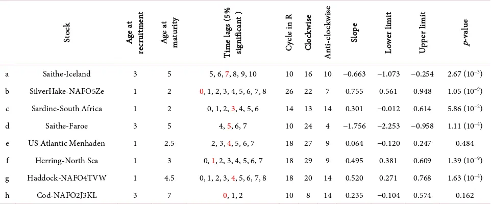
DOI: 10.4236/oalib.1103897 16 Open Access Library Journal Table 1. Basic biological parameters and the results obtained from this analysis for each of the eight stocks. Red shows the highest value of the cross-correlation between ln R* and ln SSB*.

St ock A ge a t re cru itm en t A ge a t m atu rity Ti m e l ag s ( 5% si gn ifi ca nt ) C yc le in R C lo ck w ise A nt i-c lo ck w is e Sl op e Lo w er li m it U pp er li m it p-va lue

a Saithe-Iceland 3 5 5, 6, 7, 8, 9, 10 10 16 10 −0.663 −1.073 −0.254 2.67 (10−3₎

b SilverHake-NAFO5Ze 1 2 0, 1, 2, 3, 4, 5, 6, 7, 8 26 22 7 0.755 0.561 0.948 1.05 (10−9₎

c Sardine-South Africa 1 2 0, 1, 2, 3, 4, 5, 6 14 13 14 0.301 −0.012 0.614 5.86 (10−2₎

d Saithe-Faroe 3 5 4, 5, 6, 7 10 24 4 −1.756 −2.253 −0.958 1.11 (10−4₎

e US Atlantic Menhaden 1 2.5 2, 3, 4, 5, 6, 7 18 27 9 0.064 −0.120 0.247 0.484 f Herring-North Sea 1 3 0, 1, 2, 3, 4, 5, 6, 7 18 29 9 0.495 0.381 0.609 1.39 (10−9₎

g Haddock-NAFO4TVW 1 4.5 0, 1, 2, 3, 4, 5, 6, 7, 8 18 20 14 0.520 0.271 0.768 1.63 (10−4₎

h Cod-NAFO2J3KL 3 7 0, 1, 2 10 8 14 0.235 −0.104 0.574 0.162

Figure 5(d) shows the case of Saithe in Faroe. The first and second vertexes were observed around 1967 and 1984, respectively. The significantly positive values of the auto-correlation of ln R* were distributed from −2 to 2. That is, half of the cycle of environmental conditions was estimated to be 5 years, and the

cycle of environmental conditions was estimated to be about 10 years. Figure

5(e) shows the case of US Atlantic Menharden. The first and second vertexes

were observed around 1958 and 1975, respectively. The significantly positive values of the auto-correlation of ln R* were distributed from −4 to 4. That is, half of the cycle of environmental conditions was estimated to be 9 years, and the cycle of environmental conditions was estimated to be about 18 years.

Figure 5(f) shows the case of herring in the North Sea. The first and second vertexes were observed around 1963 and 1985, respectively. The significantly positive values of the auto-correlation of ln R* were distributed from −4 to 4. That is, half of the cycle of environmental conditions was estimated to be 9 years, and the cycle of environmental conditions was estimated to be 18 years. Figure 5(g) shows the case of Haddock in NAFO4TVW. The first and second vertexes were observed around 1963 and 1977, respectively. The significantly positive values of the auto-correlation of ln R* were distributed from −4 to 4. That is, half of the cycle of environmental conditions was estimated to be 9

years, and the cycle of environmental conditions was estimated to be 18 years.

Fig-ure 5(h) shows the case of Cod-NAFO2J3KL. This case is easier to discuss using the valleys. The first, second and third valleys were observed around 1971, 1976 and 1984, respectively. The significantly positive values of the auto-correlation of ln R* were distributed from −2 to 2. That is, half of the cycle of environmental tions was estimated to be 5 years, and the average cycle of environmental

condi-tions was estimated to be 10 years. Table 1 summarizes the results mentioned

DOI: 10.4236/oalib.1103897 17 Open Access Library Journal the length of the environmental cycle, blue arrows are dominant, and if the age at maturity is less than half the length of the environmental cycle, red arrows are

dominant [10] [14] [16] [17]. In the case of Saithe in Iceland, the age at maturity

is equal to half of the length of the environmental cycle, and so the dominant color of the arrows is not clear; in practice, the numbers of blue and red arrows were not much different. In cases (b), (e), (f) and (g), the age at maturity was less than half of the environmental cycle, and the red arrows were more dominant than the blue arrows. In case (c), the age at maturity was less than half the length of the environmental cycle; however, the number of red arrows was smaller than the number of blue arrows, although the difference was not large. In case (d), the age at maturity was equal to half of the length of the environmental cycle; how-ever, the number of red arrows was much higher than the number of blue ar-rows. These two cases were the exceptions to the loop theory. In the case of cod in NAFO2J3KL, the age at maturity was much greater than half of the length of the environmental cycle, and the number of blue arrows was greater than the number of red arrows.

3.3. The Slope of the Regression Line Drawn on the SRR

Figure 6 also shows the slope of the regression line as a green line drawn on the SRR plain. The slopes seem to have some relationship with their ages at maturi-ty. In the stocks for which the age at maturity was low, the slopes were positive. Figure 6(b), Figure 6(f), and Figure 6(g) seem to show such cases. In the stocks for which the age at maturity was high and was close to half the length of the cycle of environmental factors, the slopes were close to zero. Cases (c) and (e) seem to be cases of this. In cases (a) and (d), the ages at maturity were high, and the slopes of the regression lines were both negative. In contrast, in case (h), the age at maturity was extremely large, even though the slope of the regression line was not negative but almost zero. These results were slightly different from those that the loop theory forecasted.

Figure 7 shows the relationship between the slope of the regression lines and the age at maturity for 36 stocks. Eight stocks were estimated in this study and

DOI: 10.4236/oalib.1103897 21 Open Access Library Journal Figure 6. Stock-recruitment relationship for stocks (a) to (h), respectively. That is, a pair consisting of ln Rt and ln SSBt−d, i.e., (ln SSBt−d, ln Rt), is plotted. The figures on the graph

DOI: 10.4236/oalib.1103897 22 Open Access Library Journal Figure 7. Relationship between the slope of the regression line (b) drawn on the SRR plane and the age-at-maturity (m). The slope was estimated as b = 0.995 − 0.211 m. The 95% confidence intervals of the slopes were (−0.343, −0.097). That is, the negative slope is statistically significant at a 95% significance level.

and were plotted with black closed circles, and 2 stocks were estimated by

Saku-ramoto [14] and were plotted with black open circles. The slope of the regression

line was

0.995 0.211 .

b= − m

Here, b and m denote the slope of the regression line and the age at maturity,

respectively. The 95% confidence intervals of the slopes were (−0.343, −0.097),

and those of the intercept were (0.541, 1.450). The p-values of the slope and

in-tercept were 1.02 × 10−4 _{and 2.70 × 10}−3_{, respectively. That is, a significant}

nega-tive relationship was detected between the slopes of the regression lines and the age at maturity. This result coincided well with the results of the simulations

proposed by Sakuramoto [14].

4. Discussion

4.1. Clockwise or Anticlockwise Loops in the SRR

DOI: 10.4236/oalib.1103897 23 Open Access Library Journal important factor in controlling the fluctuation, and the true mechanism that controls SRR must be explained in another way. In other words, the mechanism by which clockwise loops or anticlockwise loops commonly appear in SRR can-not be explained by the density-dependent effect.

In this study, I did not specify the typical environmental factors that con-trolled the fluctuations in the eight stocks analyzed in this paper, as an analysis of those factors would have been too time-consuming. However, some examples have already been investigated. For instance, the environmental factors that would control the fluctuations in the Pacific stock of Japanese sardines were

al-ready investigated in detail [14] [22] [23], as were those of Pacific bluefin tuna

[14]. The main environmental factors found in those analyses were the index of

Arctic Oscillation (AO) by month and the index of Pacific Decadal Oscillation

(PDO) by month. Hasegawa et al. [24] also investigated the relationship between

the catch fluctuation of pink salmon and environmental factors, and using the AO and/or PDO, they showed that the loop theory could be applied this stock. Therefore, I strongly believe that specifying the environmental factors that affect the population fluctuations of the eight stocks analyzed in this paper is also possible. In the next step in my future research, I will specify the environmental factors for each of the eight stocks.

In this study, I applied the loop theory to the data that Myers et al. analyzed in

1994 [19], and showed that the results were the same as those shown in Sakura-moto [14] [15] [16] and Tanaka et al. [17]. That is, the clockwise or anticlock-wise loops in SRR emerged depending on the age at maturity, and the slope of the regression line had a negative slope with the age at-maturity. When age at maturity was high, however, there were two exceptions in this study. In particu-lar, the age at maturity of Saithe in Faroe is 5 years, which is relatively high; however, the number of line segments with a clockwise direction was greater than the number with an anticlockwise direction.

It is difficult to explain in detail why the exception occurred at this stage;

however, some of the possible reasons include the following. Hasegawa et al.

[24] noted that even when the age at maturity is low, the SRR can show

DOI: 10.4236/oalib.1103897 24 Open Access Library Journal loops and the stock born in the even-numbered years had anti-clockwise loops. These two stocks have the same age at maturity; that is, they come back to their native river for spawning 2 years after they were spawned. However, it was found that the catches in odd and even years had a significant negative tion with each other with 10% significant level. Thus, when a negative correla-tion was present, the clockwise loops changed to anti-clockwise loops. Therefore, the direction of the loops can be strongly influenced not only by the age at ma-turity and the cycle of environmental factors, but also by species interactions. Therefore, we should further investigate the biological relationships between the stocks.

The age at maturity seems to be determined on a species-by-species or stock-by-stock basis. However, even in the same species, the environmental condi-tions that affect the population fluctuacondi-tions are different in different habitats. Fur-ther, even in the same habitat, the length of the environmental cycle itself changes era by era. Therefore, the number of line segments that with a clockwise or anti-clockwise direction differed by stock and by era. In the case of Saithe Faroe, the age at maturity is high, 5 years; however, the number of line segments that show the clockwise loop is much greater than the number of line segments that show the anti-clockwise loop. In order to discuss these phenomena, we should further ex-amine the environmental conditions and species interactions for each stock.

The results obtained for 24 stocks that live around Japan [17] coincided with

the results obtained in this study. That is, although the construction mechanism of the SRR is complex, loops always appear for all SRRs. The areas where the

stocks that were analyzed by Tanaka et al. live [17], and the areas where the

stocks that were examined in this paper live were quite different, but the essen-tial results coincided well.

4.2. Slope of the Regression Lines in SRR

Sakuramoto noted that the slopes of the regression lines adapted for SRR were

determined by the age at maturity and the cycle of environmental factors [14]

[16]. When the age at maturity is low enough compared to the cycle of

environ-mental factors, the slope estimated by a simple regression method, in which

ln(Rt) is plotted against ln(SSBt−d), shows a positive value, although the slope is

statistically less than unity. When the age at maturity is close to half of the length of the cycle of environmental factors, the slope of the regression line is close to zero and is not statistically different from zero. Furthermore, the age at maturity becomes greater than the length of half of the cycle of environmental factors, the

slope of the regression line becomes negative. Sakuramoto [14] showed that the

com-DOI: 10.4236/oalib.1103897 25 Open Access Library Journal

principle of which is shown in Figure 3(a). Generally, the age at recruitment is

lower than the age at maturity, because immature fish are commonly harvested.

This clearly indicates d ≤ m. Figures 1-3 show that the SRR corresponds to the

R-R relationship. In Model 2, the SRR was expressed by R_{t m d+ +} =α

(

)

When m = 0, and d = 0, the SRR becomes R_t = +

(

)

( )

(

)

( )

ln S_t

+ _{. This indicates that the slope of SRR becomes unity. Similarly, in}

Mod-el 3, the SRR was expressed by Rt m d+ + =

α

β

(

ω

(

)

)

m = 0, and d = 0, the SRR becomesRt = +1

β

(

ω

( )

)

( )

(

(

( )

)

)

( )

ln Rt =ln +β n ω t +ln St . Then, the slope becomes unity.

I set a rule that determines the direction of the line segment from year t to

year t + 1; however, this rule is only a tentative example. A much more

reasona-ble rule must exist; however, the aim of making the rule is to avoid doing the de-finition arbitrarily. In any case, if someone determines the direction of the line without any rule, the results will not be very different.

Hilborn and Stokes [20] strongly warned the use of the unfished biomass B

un-fished to determine the reference points as follows. The standard approaches to

biomass reference points in the United States and Australia fail to make clear

that they are tied to an almost unknowable quantity, the unfished biomass B

un-fished. The target and limits for fisheries management based on historical stock

sizes and stock productivity have the advantage that they are based on expe-rience, are easily understood, and are not subject to the vagaries of model as-sumptions. The results of this paper strongly support the warning noted by

Hil-born and Stokes [20] from a different point of view.

In the scientific committee of the International Whaling Commission, major discussions and simulation studies have been conducted for more than 5 years in

order to develop a revised whale management procedure [27]. Tanaka [28]

pro-posed a new management procedure that did not assume any population model; this procedure has been called the “model independent fisheries resources

man-agement approach”. Using this theory, Sakuramoto and Tanaka [29] proposed a

simulation model that could manage baleen whale stocks without any

popula-tion model, and without any parameters, such as MSY, BMSY and B0, etc. That

simula-DOI: 10.4236/oalib.1103897 26 Open Access Library Journal tion program used the catch per unit of effort (CPUE) as the relative value of population abundance. The procedure commenced using two indexes: the present CPUE level compared to the target CPUE level, and the increasing or decreasing trend of the CPUE. If the present CPUE is lower than the target CPUE, the catch quota is reduced and vice versa. Further, if the CPUE shows an increasing trend, the catch quota is increased, and vice versa. The target CPUE can be determined, for instance, as follows: if the CPUEs of 10 to 15 years ago were reasonable, the average CPUE for those years can be used as the target level for the management. When this procedure is applied to actual fish stocks, very detailed simulation trials should be done to determine which parameters are

reasonable, by species. However, previous studies [27] [29] showed that the

re-sults of this procedure were acceptable. Therefore, I strongly emphasize that

empirical reference points should be used, not B0, Bunfished and BMSY, the scientific

basis of which is unclear.

5. Conclusions

The results elucidated in this paper can be summarized as follows:

1) Loop theory can be applied to the eight stocks that Myers et al. [19]

inves-tigated.

2) When the age at maturity was low enough compared to the length of the cycle of the environmental factors, clockwise loops were dominant, and when the age at maturity was high compared to the length of the cycle of the environ-mental factors, anticlockwise loops were dominant.

3) The slope of the regression line for SRR had a negative correlation with the age at maturity. When the age at maturity was low, the slope was positive but less than unity. When the age at maturity became high, the slope decreased to zero. In this case, no relationship was observed between R and SSB.

4) Reference points derived from the traditional SRR model do not have any

scientific basis. B0, Bunfished and BMSY should not be used as the reference points.

5) Empirical reference points should be used, as Hilborn and Stokes [20]

em-phasized.

Acknowledgements

I greatly appreciated Dr. Myers and his group for their contributions to produc-ing the database from which many kinds of fish stock data can easily obtained. The database has played a very important role in fisheries sciences and it will al-so play an important role in the future. The study could only be done thanks to this database. I greatly appreciate Dr. Myers and his group for their great con-tributions. I also thank Drs. M. Melnychuk and S. Suzuki and Ms. K. Tanaka for their useful comments.

Competing Financial Interests

DOI: 10.4236/oalib.1103897 27 Open Access Library Journal (1994) In Search of Thresholds for Recruitment Overfishing. ICES Journal of

Ma-rine Science, 51, 191-205.https://doi.org/10.1006/jmsc.1994.1020

[5] Baumgartner, T.R., Soutar, A. and Ferreira-Bartrina, V. (1992) Reconstruction of the History of Pacific Sardine and Northern Anchovy Populations over the Last Two Millennia from Sediments of the Santa Barbara Basin, California. CalCOFI

Reports, 33, 24-40.

[6] Ravier, C. and Fromentin, J.M. (2001) Long-Term Fluctuations in the Eastern At-lantic and Mediterranean Bluefin Tuna Population. ICES Journal of Marine Science, 58, 1299-1317. https://doi.org/10.1006/jmsc.2001.1119

[7] Ricker, W.E. (1954) Stock and Recruitment. Journal of the Fisheries Research Board

of Canada, 11, 559-623.https://doi.org/10.1139/f54-039

[8] Beverton, R.J.H. and Holt, S.J. (1957) On the Dynamics of Exploited Fish Popula-tions Fishery InvestigaPopula-tions. Series II 19, 1-533, Her Majesty’s Stationery Office, London.

[9] Shepherd, J.G. (1982) A Versatile New Stock-Recruitment Relationship for Fisheries and the Construction of Sustainable Yield Curves. Journal du Conseil International

Pour Exploration de la Mer, 40, 67-75. https://doi.org/10.1093/icesjms/40.1.67

[10] Sakuramoto, K. (2005) Does the Ricker or Beverton and Holt Type of Stock-Recruitment Relationship Truly Exist? Fisheries Science, 71, 577-592.

https://doi.org/10.1111/j.1444-2906.2005.01002.x

[11] Sakuramoto, K. (2013) A Recruitment Forecasting Model for the Pacific Stock of the Japanese Sardine (Sardinops melanostictus) That Does Not Assume Densi-ty-Dependent Effects. Agricultural Sciences, 4, 1-8.

https://doi.org/10.4236/as.2013.46A001

[12] Sakuramoto, K. (2014) A Common Concept of Population Dynamics Applicable to Both Thrips imaginis (Thysanoptera) and the Pacific Stock of the Japanese Sardine

(Sardinops melanostictus). Fisheries and Aquatic Sciences,140-151.

[13] Sakuramoto, K. (2015) Illusion of a Density-Dependent Effect in Biology.

Agricul-tural Sciences, 6, 479-488.https://doi.org/10.4236/as.2015.65047

[14] Sakuramoto, K. (2015) A Stock-Recruitment Relationship Applicable to Pacific Blu-efin Tuna and the Pacific Stock of Japanese Sardine. American Journal of Climate

Change, 4, 446-460.https://doi.org/10.4236/ajcc.2015.45036

[15] Sakuramoto, K. (2016) A Simulation Model of the Spawning Stock Biomass of Pa-cific Bluefin Tuna and Evaluation of Fisheries Regulations. American Journal of

Climate Change, 5, 245-260. https://doi.org/10.4236/ajcc.2016.52021

DOI: 10.4236/oalib.1103897 28 Open Access Library Journal

Open Access Library Journal, 3, e3112.https://doi.org/10.4236/oalib.1103112

[17] Tanaka, K., Suzuki, N. and Sakuramoto, S. (2017) Clockwise Loops and Anticlock-wise Loops Observed in a Stock-Recruitment Relationship. Open Access Library

Journal, 4, e3688.https://doi.org/10.4236/oalib.1103688

[18] Myers, R.A. http://ram.biology.dal.ca/~myers/data.html

[19] Myers, R.A., Rosenberg, A.A., Mace, P.M., Barrowman, N. and Restrepo, V.R. (1994) Is Search of Thresholds for Recruitment Overfishing? ICES Journal of

Ma-rine Science, 51, 191-205.https://doi.org/10.1006/jmsc.1994.1020

[20] Hilborn, R. and Stokes, S. (2010) Defining Overfishing Stocks: Have We Lost the Plot? Fisheries, 3, 113-120. http://www.fisheries.org

https://doi.org/10.1577/1548-8446-35.3.113

[21] https://www.sanbi.org/creature/South%20African%20sardine

[22] Shimoyama, S., Sakuramoto, K. and Suzuki, N. (2007) Proposal for Stock-Recruitment Relationship for Japanese Sardine Sardinops melanostictus in the North-Western Pacific. Fisheries Science, 73, 1035-1041.

https://doi.org/10.1111/j.1444-2906.2007.01433.x

[23] Sakuramoto, K., Shimoyama, S. and Suzuki, N. (2010) Relationships between Envi-ronmental Conditions and Fluctuations in the Recruitment of Japanese Sardine,

Sardinops melanostictus, in the Northwestern Pacific. Bulletin of the Japanese

So-ciety of Fisheries Oceanography, 74, 88-97.

[24] Hasegawa, S., Suzuki, H. and Sakuramoto, K. (2015) Performance of Deming and Passing Bablok Regression Analysis in Detecting Proportionality in the Stock-Recruitment Relationship. Asian Fisheries Science, 28, 102-116.

[25] Pacific Bluefin Tuna Working Group (PBFWG) (2014) Stock Assessment of Pacific Bluefin Tuna 2014. Report of the Pacific Bluefin Tuna Working Group. Interna-tional Scientific Committee for Tuna and Tuna-Like Species in the North Pacific Ocean, 1-121.

[26] Mesnil, B. and Rochet, M.J. (2010) A Continuous Hockey Stick Stock-Recruit Mod-el for Estimating MSY Reference Points. ICES Journal of Marine Science, 67, 1780-1784.https://doi.org/10.1093/icesjms/fsq055

[27] International Whaling Commission (1991) Report of the Subcommittee on Man-agement Procedures. Report International Whaling Commission, 41, 90-124. [28] Tanaka, S. (1980) A Theoretical Consideration on the Management of a

Stock-Fishery System by Catch Quota and on Its Dynamic Properties. Bulletin of

the Japanese Society for the Science of Fish, 46, 1477-1482.

https://doi.org/10.2331/suisan.46.1477

[29] Sakuramoto, K. and Tanaka, S. (1989) A Simulation Study on the Management of Whale Stocks Considering Feedback Systems. Report International Whaling