The Role of Information in the Discrepancy Between Average Prices and Expectations

Munich Personal RePEc Archive

The Role of Information in the

Discrepancy Between Average Prices and

Expectations

Barbosa, António

ISCTE - Instituto Universitário de Lisboa

December 2019

Online at

https://mpra.ub.uni-muenchen.de/97416/

The Role of Information in the Discrepancy Between

Average Prices and Expectations

António Barbosa

Department of Finance

ISCTE-IUL - Instituto Universitário de Lisboa

This version: December 2019

Abstract

In this paper I show how the existence of short-term trading causes a diver-gence between the average price and the average expectation of the fundamen-tal value by embedding higher-order expectations –expectations of expectations of expectations...– into prices. Short-term trading arises when investors receive private information and (i) either net supply mean reverts or (ii) the release of additional information related to existing information is combined with residual uncertainty. Mean-reversion of net supply, brings the average expectation closer to the fundamental value than the average price after the release of private informa-tion. By the contrary, residual uncertainty and an incoming release of information brings the average price closer to the fundamental value than the average expec-tation before the new information is released. When both (i) and (ii) are present, the average expectation tends to be closer to the fundamental value than the av-erage price in the periods immediately after information releases, but the opposite happens in the periods immediately before information releases.

∗

1

Introduction

In a static setting, the equilibrium price of a risky asset equals the average expecta-tion of market participants about its terminal payoff, adjusted for a risk premium. If the asset is, on average, in zero net supply, there is no risk premium and the average price coincides with the average expectation. However, this is not necessarily true in a dynamic setting. If investors engage in short-term trading, they care about inter-mediate prices, which embeds higher-order expectations – expectations of expectations of expectations...– into prices.1

This creates a wedge between the average price and the average first-order expectation of the liquidation value because the law of iterated expectations fails for average expectations (Allen et al., 2006).

Allen et al. (2006) show that, in a dynamic economy populated by short-term in-vestors, with no residual uncertainty and i.i.d. noise trade, short-term trading leads to over-reliance on public information when investors have private information.2

This means that the average expectation of the liquidation value are closer to the fundamen-tal value than the average price. In their own words,

“Now suppose that the individual is asked to guess what the average ex-pectation of the asset’s payoff is. Since he knows that others have also observed the same public signal, the public signal is a better predictor of average opinion; he will put more weight on the public signal than on the private signal. Thus if individuals’ willingness to pay for an asset is related to their expectations of the average opinion, then we will tend to have asset prices overweighting public information relative to the private information.”

and go as far as saying that (my emphasis)

“Thus any model where higher-order beliefs play a role in pricing assets will deliver the conclusion that there is an excess reliance on public information.”

Cespa and Vives (2012) show that, contrary to Allen et al.’s bold claim, over-reliance on public information is not an universal result when higher-order beliefs are embedded in prices. This is true even for an economy populated by short-run investors as in Allen et al., 2006 if noise trade is not i.i.d.. In an economy populated by long-run

1

Higher-order expectation are imbedded into prices because the price at the second to last trading date depends on the average expectation of the price at the last trading date, which in turn depends on the average expectation of the terminal payoff, and so on. Thus, prices exhibit beauty contest features, as envisioned by Keynes (1936).

2

investors, Cespa and Vives (2012) claim that whether over-reliance or under-reliance on public information obtains, depends on the parameters of the model. Specifically, over-reliance on public information is obtained when residual uncertainty is low, and net supply changes are strongly correlated. Otherwise, under-reliance on public information is obtained.

My contribute to this recent literature is to identify the crucial role of the infor-mation environment on over- and under-reliance on public inforinfor-mation when investors have long-run investment horizons. Cespa and Vives (2012) fail to identify the role of the information environment for two reasons: first, they always assume that investors observe private exogenous information at all periods; second, they consider only two trading dates.3

By relaxing the first assumption, I show that under-reliance on public information occurs only if additional exogenous information related to existing private information is known to be released in the future. By expanding the model to allow more than two trading dates, I show that over- and under-reliance on public information can arise in the same economy at different dates: over-reliance on public information is most likely to occur in the periods immediately after the release of exogenous in-formation; in turn, under-reliance on public information tends to occur in the periods immediately preceding the release of additional exogenous information.

The intuition is the following. On average, investors believe that the price reaction to the initial release of private exogenous information is due not only to a change in informed demand, but also to a change in the liquidity driven demand away from zero. If noise trading is persistent, future price changes are unpredictable, and there is no short-term trading. In this case the average price and expectation coincide. But if noise trading mean reverts, investors can forecast future net supply levels and prices. This creates a short-term opportunity to profit from liquidity traders as they exit the market, and makes investors less eager to build their long-run position immediately. That is, short-term trading diverts attentions from the long-run. As a result, less of the private information makes its way into prices, which causes the average price to be further away from the fundamental value than the average expectation of the liquidation value. That is, prices over-rely on public information.

In turn, when investors expect the release of additional exogenous information re-lated to their private information, they use their private information more aggressively to bet on the price impact of the incoming information. This impounds more of the existing information into prices, bringing the average price closer to the fundamental

3

value than the average expectation. In other words, prices under-rely on public infor-mation. Using Allen et al.’s intuition, on the one hand, all investorsobserved the same public information (the common prior), and a private signal. Although investors know what the public information was, they can only make an inaccurate estimate of what other investors’ private signals might have been. Hence the tendency to over-rely on public information. But, on the other hand, all investors will observe another private signal related to the private signal already observed. Since the incoming private signal can be forecasted with the previously observed private signal, investors will rely more heavily on their own private signal and less on the public signal when forming beliefs about others’ beliefs. Allen et al. (2006) do not obtain this result because in their model (i) there is no residual uncertainty and (ii) there is mean-reversion of net supply.

When net supply mean reverts and there is an additional release of information, the effect of the former tends to dominate in the periods closer to the initial relase of private information, because this is when the net supply level is believed to be further away from its unconditional mean; whereas the effect of the latter tends to dominate in the periods closer to the relase of the new information, for that is when expected price impact of the new information is believed to be strongest. This means that prices tend to over-rely on public information in the periods following information releases and under-rely on public information in the periods leading to information releases.

In addition, I show that over-reliance on public information is one-to-one with the average expectation being closer to the fundamental value than the average price only when all exogenous information is based on the same underlying signal. When that is not the case, it is possible for the average price to be the best predictor of the fundamental value even though prices over-rely on public information.

Finally, I point out that the price pattern preceding the release of additional ex-ogenous information resembles the leakage of inside information, and that prices tend to be more informative about the fundamental value in periods of high price volatility. The latter backs the traditional view of a more volatility market as one where more information is gathered (e.g. Admati and Pfleiderer, 1988) and it is in contrast with the results of Cespa (2002).

This paper is closely related to Barbosa (2011) in that they share the same model. However, the set of questions analyzed are clearly distinct. In Barbosa (2011) I study the time-series of average prices and expectations following the release of private exogenous information. Here, I study how the average price compares to the average expectation at any given point in time.

for the equilibrium price and demand functions in Section 3. In Section 4 I study how the average price diverges from the average expectation of the liquidation value and from the fundamental value when there is a single signal underlying all releases of exogenous information. In Section 5 I analyze how different underlying signals change those results. In Section 6 I discuss additional implications of the model, and Section 7 concludes. All proofs and additional discussion are provided in the Appendix.

2

The Model

I will use the same model developed in Barbosa (2011). For convenience, I will describe it here once again. There is one risky asset and one riskless asset traded at dates

1,2, ..., T −1. The riskless asset has a perfectly elastic supply and a zero net rate of

return. The risky asset is liquidated at date T, payingv ∼N(0, σ_v2). The date t risky asset’s per capita net supply (θt) is random, due to noise/liquidity driven demand, and

follows theAR(1) process

θt =ρθt−1+εθ,t, εθ,t ∼N 0, σθ2

, t= 1,2, ..., T −1 (1)

with 0≤ρ≤1 and θ0 = 0.

There is a continuum of risk averse investors of measure 1, indexed byi. All investors have CARA preferences over their terminal wealth (Wi

T) with the same coefficient of

risk aversion (α). At every date t, investor ichooses the risky asset demand (Xi t) that

maximizes his expected utility conditional on the information currently available to him (Fi

t) by solving

max

Xi t

Eh−e−αWTi|Fi

t

i

s.t. Wti+1 =Wti+Xti(Pt+1−Pt), (2)

where Pt is the date t risky asset’s price. Investors have homogeneous prior beliefs,

v ∼N(0, σ_v2)and θ0 = 0, denoted by F0.

There are n underlying signals for the liquidation value v,

s=v1_{(n×1)+εs, εs∼N} 0_{(n×1),Σs, (3)}

Investors do not observe these underlying signals directly. Instead, at every date t

investors observe a private version of those underlying signals:

˜

si_t=s+εi_t, εi_t ∼N 0_{(n×1),Σ˜s,t, (4)}

with private noise εi

t independent across i and t and with independent components

(i.e. Σ˜s,t is restricted to be diagonal). The set of covariance matrices{Σ˜s,t: 1≤t < T}

defines the timing of exogenous information release: the j-th diagonal entry of Σ˜s,t is

equal to ∞ if there is no signal for the j-th underlying signal at date t; and less than

∞otherwise.

The total information available to investori and the common information available to all investors are defined as

Fti =

F0,s˜iτ, Pτ :τ = 1, ..., t ,Ftc ={F0, Pτ :τ = 1, ..., t},

respectively. Unless it is explicitly stated otherwise, all random variables are indepen-dent of each other and across time.

With the model laid down, I can now define three concepts that I will use throughout the paper: residual uncertainty, exogenous information and endogenous information. Residual uncertainty is the amount of uncertainty that would persist after the direct observation of the underlying signals. Therefore residual uncertainty is a function of the covariance matrixΣs. If at least one diagonal entry ofΣs is zero, the corresponding

underlying signal coincides with the liquidation value, and there is no residual uncer-tainty.

The second concept, exogenous information, is defined as the information directly obtained from the observation of_s˜i_{t. I say that there is exogenous information at date}

t if at least one of the diagonal entries of Σ˜s,t is less than ∞.

produced information from the observation of the sequence of prices that follow the initial release of private exogenous information.

3

Equilibrium

The full details on how to determine the equilibrium price and demand functions are provided in Barbosa (2011). To avoid unnecessary repetition, here I will only present the price and demand functions without further details on how to derive them.

Theorem 1. In a linear equilibrium, the price function is given by

Pt=

ˆ

K−p_t

E[s|Ftc] +pts+pθ,tθt=

ˆ

K−p_t

E[s|Ftc] +ξt (5)

where ξt≡pts+pθ,tθt and the demand function is given by

X_ti = 1

αQtψt, t= 1,2, ..., T −1 (6)

where ψ_t is a vector of state variables defined as

ψ_t≡

     

1 E(s|Fi

t)

E(s|Fc t)

E(θt|Fti)

     

.

The demand of investor i is a linear function of the expectations of the vector of underlying signals s and the net supply level θt conditional on his information set

Fi

t. This implies that, once investors observe private exogenous information about one

underlying signal, and until that underlying signal is revealed to them, every investor will demand a different amount of the risky asset. As shown in theorem 2 of Barbosa (2011), expectations conditional onFi

t are a linear function of prior beliefs, information

extracted from prices and investori’s private exogenous information. Since the private noise in exogenous information (εi

t) is normally distributed, it follows that expectations

conditional on Fi

t are also normally distributed across investors. And so is investor’s

demand.

Market clearing requires that the average demand matches the per capita supply for the asset, R_iXi

t = θt∀t. The existence of a continuum of investors with conditionally

normally distributed demands implies that there is one investor whose demand is exactly equal to the average demand. I refer to this investor as the average investor (AI). It follows that the market clears if and only if the demand of the AI equals the per capita net supply. This allows us to simplify the analysis in the next sections by focusing on this representative investor. The next corollary identifies the AI, at date

t, as the investor whose all past and current private signals exactly coincide with the corresponding underlying signals.

Corollary 3. The market clears at date t if and only if the demand of the investor who observes _s˜i_{τ =s, ∀τ ≤ t, the average investor (AI), matches the per capita asset’s}

net supply. In addition, the beliefs of the AI coincide with the average beliefs across investors, i.e. _E v|FAI

t

=_Ei[E(v|Fti)].

The demand function (6), although parsimonious, is not particularly intuitive. The next lemma tells us that the risky asset demand can be written as a linear function of the expectations about all future price changes; or as a linear function of the short-term myopic demand and all expected future non-myopic demands (the hedging demand).

Lemma 4. The demand function can also be written as

X_ti = 1

α

T−t

X

τ=1

χQτ,tE

∆Pt+τ|Fti

, (7)

Xti =

1

α

T−t

X

τ=1

ξτ,tE

Pt+τ −Pt|Fti

, (8)

Xti = φ

Q

1,tXe i t +

T_X−t−1

τ=1

φQτ,tE

Xt+τ|Fti

, (9)

where ∆Pt+τ ≡ Pt+τ −Pt+τ−1 is the one-period return and Xeti ≡

E(∆Pt+1|F_ti)

αV ar(∆Pt+1|F_ti) is the

short-term myopic demand. Moreover,χQ_1,t >0andφQ_1,t >0. All parameters are defined in Appendix A.2.

makes the next period expected return negatively correlated with all subsequent ex-pected returns. In that case, hedging future positions requires the investor to take today a position of the same sign of their expected future short-term position (i.e., the same sign of the expected return), and so χQτ,t > 0 for τ ≥ 1. Expected returns

may become positively correlated, leading to χQτ,t < 0, in the period before exogenous

information is released. But only if that exogenous information significantly reduces the uncertainty about the liquidation value.

The following assumption relates the magnitude of short-term demand with that of hedging demand.

Assumption 5. The following holds: χQ_1,t >P_τT₌₂−tχQτ,t∀t . That is, demand is strictly

positive (negative) whenever the expected price change over the next period is positive (negative) and all future expected prices are never below (above) the current price.

This means that if the price change over the next period has the same magnitude but the opposite sign of the price change from the next period all the way to the liquidation date, then short-term demand dominates the hedging demand and the overall demand has the same sign of the short-term demand. Note that, in this case, the asset has only upside or only downside potential, and so it is expectable that investors take advantage of it with a short or long position in the asset, respectively. However intuitive this assumption might be, it does not hold true for generic return processes. In Appendix D I discuss the validity of this assumption for the endogenous return process implied by the model used in this paper.

4

Discrepancy between Average Prices and

Expecta-tions: The Case of a Single Underlying Signal

I will now use the model introduced in the previous sections to study in which circum-stances and in which direction the average price differs from the average expectation of the liquidation value. In this section, the focus will be on the case of a single underly-ing signals. Note that, even though there is a single underlying signal, investors may observe several private signals based on that same underlying signal at different dates. The case where investors observe private signals based on multiple underlying signals is addressed in the next section.

level and investors) expectation of the liquidation value”. I will also refer to the average expectation of the liquidation value simply as the average expectation.

This setup with a single underlying signal is the closest to the one used by Cespa and Vives (2012). The main difference relative to their work is that I relax the assumption that investors observe exogenous information forsin every period (i.e. I allowΣs,t˜ =∞ at some dates t), and consider more than 2 trading dates (T >3). The former allows me to identify the existence of additional exogenous information, following an initial release of private exogenous information, as a crucial factor to have prices closer to fundamentals than expectations. In turn, the latter allows me to find that the prices can be closer to fundamentals in some periods, while expectations are closer to fundamentals in other periods.

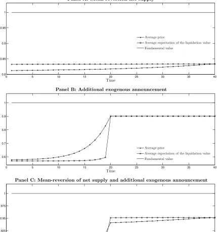
I show that, following an initial release of private exogenous information, either (i) mean-reversion of net supply or (ii) a combination of residual uncertainty with an additional release of exogenous information create a discrepancy between prices and expectations. In both cases, the root cause for this discrepancy between prices and expectations is the existence of short-term speculative trading opportunities. Moreover, I show that prices differ from expectations in a different way depending on whether (i), (ii) or both occur. Mean-reversion of net supply tends to bring expectations closer to fundamentals than prices after the release of private exogenous information. By the contrary, residual uncertainty and an incoming release of exogenous information tends to make prices closer to fundamentals than expectations before the new information is released. Figure 1 previews these results.

Without loss of generality, I assume henceforth that the initial private exogenous information is released at date 1. Since there is only one underlying signal, the funda-mental value of the risky asset (F V) is defined as the expected liquidation value given the direct observation of the underlying signal, and is independent oft. The next lemma provides the expressions for the fundamental value, average price (Eθ(Pt)) and average

expectation of the liquidation value (Eθ,i[E(v|Fti)]≡Eθ

E v|FAI t

). All averages are over the net supply level and investors, and conditional on the underlying signals.

0 5 10 15 20 25 30 35 40 0.8

0.85 0.9 0.95 1

Panel A: Mean-reversion net supply

Time

Average price

Average expectation of the liquidation value Fundamental value

0 5 10 15 20 25 30 35 40

0.6 0.7 0.8 0.9 1

Panel B: Additional exogenous announcement

Time

Average price

Average expectation of the liquidation value Fundamental value

0 5 10 15 20 25 30 35 40

0.875 0.9 0.925 0.95 0.975 1

Panel C: Mean-reversion of net supply and additional exogenous announcement

Time

Average price

Average expectation of the liquidation value Fundamental value

Figure 1: Discrepancy between the average price, the average expectation of the liqui-dation value and the fundamental value. This figure shows the discrepancy between the average price, the average expectation of the liquidation value and the fundamental value when: there is mean-reversion of net supply (panel A); there is an incoming release of additional exogenous information (panel B); and the previous two occur simultaneously (panel C). In all cases, private exogenous infor-mation is released at date 1, and there is residual uncertainty. In panel A,ρ= 0.9andΣ˜s,20= 1010; in

panel B,ρ= 1andΣ˜s,20= 0.1; and in panel C,ρ= 0.9andΣ˜s,20= 0.1. The rest of the

expectation of the liquidation value conditional ons are given by

F V = Ksˆ

Eθ(Pt) =

ˆ

K−pt

Eθ[E(s|Ftc)] +pts

Eθ,i

E v|Fti

= Kˆ1−Γˆt

Eθ[E(s|Ftc)] + ˆKΓˆts

where Kˆ = σv2

σ2

v+σs2 and ˆ

Γt=V ar(v|Fti)

Pt k=1 σ12

i,k, σ 2

i,t ≡Σ˜s,t.

Furthermore, the following holds:

(i) The average price and the average expectation of the liquidation value are biased toward the prior belief about the liquidation value;

(ii) The average price is closer to (further away from) the fundamental value than the average expectation of the liquidation value is if and only if prices exhibit under-(over-)reliance on public information relatively to the optimal statistical weight, i.e.,

ˆ

K−pt<(>) ˆK

1−Γˆt

.

This result establishes the one to one link between the (relative) under-reliance of prices on public information and prices being the best estimator of the fundamental value when there is a single underlying signal. The less weight prices put on public information, i.e. E(st|Ftc), the less they overweight the prior belief about v, and the

closer they are to the fundamental value, compared to average expectations. A similar result is provided by Cespa and Vives (2012). However, this result is specific to the case of a single underlying signal.

4.1

The Base Case: Exogenous Information at a Single Date

and No Mean-Reversion of Net Supply

In order to understand why, and in which direction, the average price deviates from the average expectation of the liquidation value, I start by considering the simplest case: private exogenous information is availableonly at date 1 and there is no mean-reversion of net supply (ρ= 1).

liquidation date, then demand depends only on the expectation of the liquidation value and the current price, that is

X_ti = 1

αξT−t,tE v−Pt|F

i t

,

just like in the static model (in this caseξT−t,t=V ar(v|Fti)

−1 )

In the absence of the arrival of additional exogenous information, the only event with impact on prices are changes in net supply. And although prices do change every period in response to changes in net supply, they do not change in a predictable direction because there is no mean-reversion of net supply change. Therefore, the expected change in net supply and prices is zero. This means that, in every period, investors trade as if they hold their position until the liquidation date. Since, on average, the net supply level is zero, this means that the AI (the investor whose demand has to match the net supply level for the market to clear) has to demand zero. But this only happens if the price matches the AI’s expectation of the liquidation value, that is, if the price coincides with the average expectation of the liquidation value,

Eθ XtAI

= 1

αξT−t,tEθ

E v−Pt|FtAI

=Eθ(θt)

⇔ 1

αξT−t,tEθ

E v|FtAI

−Pt

= 0

⇔ Eθ(Pt) = Eθ

E v|FtAI

=Eθ,i

E v|Fti

.

Therefore, to create a discrepancy between average price and the average expecta-tion of the liquidaexpecta-tion value investors need to engage in short-term trading. This can be achieved either by introducing mean-reversion of net supply, which leads to endogenous production of information, or by allowing the arrival of additional exogenous informa-tion combined with residual uncertainty. This is the plan for the next two subsecinforma-tions and, as we will see, these two changes to the base case will cause the average price to deviated from the average expectation of the liquidation value in different directions.

4.2

Mean-Reversion of Net Supply: Endogenous Information

mean.

Obviously, when averaging over supply shocks, the net supply equals its uncondi-tional mean and there is no net supply changes. But, in this case, do investors believe that net supply is equal to its unconditional mean? The answer is no. And this is the reason why, on average, investors expect price changes that lead them to engage in short-term trading which, in turn, allows the average price to diverge from the average expectation.

To understand why, on average, investors expect net supply (and thus prices) to change when in fact it does not, we need to understand what happens when investors observe private exogenous information. To simplify the exposition, let us focus the attention on the average investor (AI). Like any other investor, the AI has two pieces of information: his private signal for s, s˜i

1 = s+εi1; and the informational equivalent to the contemporaneous equilibrium price, ξ1 = s+

pθ,1

p1 θ1.

4

However, there are three unknowns to the AI: the underlying signal s; the idiosyncratic error of his signal εi

1; and the current net supply level θ1. This means that there is an infinite number of combinations of these three unknowns that can generate the two observations: for a givens˜i, the larger the underlying signal, the smaller the error in the signal (i.e. the less positive or more negative the error is); and for a given price, the larger the underlying signal, the larger the net supply level.5

Therefore, it is impossible to learn the value of

s and θ1 with certainty at date 1. Instead, the AI has to estimate the value of these three unknowns.

The AI always observe s˜AI

1 =s, although he does not know that (since he does not know that he is the AI). And, when averaging over net supply shocks, he, like any other investor, observes ξ1 = s. However, because both signals for s are noisy, the AI gives some weight to his prior belief when forming his posterior belief about s. This means that, on average, his belief aboutsis biased toward the prior, i.e. Eθ

E s|FAI

1 <|s|. This is evident from the expression for the posterior belief aboutsderived for a 3-period model without residual uncertainty (see Barbosa, 2011),

E s|Fi

1

= 1

σ2

v0 + 1

α2_σ4

i,1σ 2

θ

ξ1+ _σ12

i,1˜ si 1 1 σ2 v + 1

α2_σ4

i,1σ 2

θ + 1

σ2

i,1

,Eθ,i

E s|Fi

1

=

1

α2_σ4

i,1σ 2 θ + 1 σ2 i,1 1 σ2 v + 1

α2_σ4

i,1σ 2 θ + 1 σ2 i,1 s

where σi,21 ≡ Σ˜s,1. As a consequence, when averaging over net supply shocks, the

4

When there is a single underlying signal it is convenient use this definition of ξt, in which case the

price function (5) becomesPt=Kˆ −ptE[s|Fc

t] +ptξt. 5

This follows from pθ,1

p1 < 0, which gives us the expected negative relation between supply and

AI believes that the net supply was different from its unconditional mean of zero, Eθ

E θ1|F1AI

6

=E(θ) = 0.6

Specifically, in the 3-period example of Barbosa (2011),

Eθ,i

E θ1|F1i

=−V ar(v|F

i

1)

ασ2

i,1σ2v

s.

However, _Eθ

E θ1|F1AI

6

= _E(θ) = 0 only if: (i) the underlying signal s does not coincide with its prior belief (s 6= 0); (ii) the prior belief aboutsis informative (σ_v2 <∞); (iii) the exogenous information received at date 1 is informative (σ2_i,1 <∞); and (iv) the underlying signal is not learned exactly at date 1 (V ar(v|Fi

1)>0, which requires that

α >0, σ_θ2 >0 and σi,21 >0, i.e. the initial exogenous information has to be private). So, because on average the AI expects a non-zero net supply level when exoge-nous information is released, he expects the net supply to mean-revert in the following periods, which has an impact on future prices. For example, following the release of exogenous information based on a positive underlying signal (s > 0), the AI believes that the net supply was negative. Then he expects the net supply to increase in the following periods as it converges to its unconditional mean of zero. And, as a result, he expects prices to decrease in the short-run. In the 3-period example,

Eθ,i

E θ2−θ1|F1i

= (1−ρ)V ar(v|F

i

1)

ασ2

i,1σv2

s >0

Eθ,i

E ∆P2|F1i

= −V ar(v|F

i

2)V ar(v|F1i) 1−ρ+α2σθ2σi,21

α2σ2_θ σ2

v+α2σθ2σi,21 σv2+σ2i,1 +α2σ2θσi,21σv2

(1−ρ)s <0.

To profit from this expectation, the AI takes a short position. However, since the net supply is in fact zero, his demand has to be zero as well, otherwise the market does not clear. This requires that his hedging demand exactly offsets his short-term speculative demand. But that cannot happen if the price equals his expectation of the liquidation value. This is very easy to see in a 3-period model. Using equation (8) we have

Xti =

1

αξ1,1E P2−P1|F

i t

+ 1

αξ2,1E v−P1|F

i t

.

6

Another way to see this is the following. Consider the realized scenario s, εi

1, θ1= (s,0,0)and

that, without loss of generality,s > 0 =E(v). This scenario implies a deviation of s from its prior mean of 0, but no deviation ofεi

1 and ofθ1from their prior means. All three variables have a normal

prior distribution and, as we know, the only point at which the probability density function of a normal distribution is zero is at its mean. This means that the alternative scenarios−ǫ, ǫ,_pp1

θ,1ǫ

When there is no residual uncertainty it can be shown that ξ1,1 and ξ2,1 are strictly positive (see Appendix A.4). The first term corresponds to the short-term demand, which in our example is negative, and the second to the hedging demand. It is clear that the market clears only if the hedging demand is positive, which means that the date 1 price has to be smaller than the expectation of the liquidation value,

Eθ

E v|FAI t

−P1

= −ξ1,1 ξ2,1E

θ

E P2−P1|FtAI

= V ar(v|F

i

2)V ar(v|F1i)

σ2

v +α2σθ2σi,21 σi,21+ρσ2v

σ2

i,1σv2

σ2

v +α2σ2θσi,21 σ2v+σi,21+α2σθ2σ2i,1σ2v

(1−ρ)s >0.

When there are more than 3 periods, the intuition remains the same. The hedging demand has to be large enough to offset the short-term speculative demand. But once again, that does not happen if the current price equals the AI’s expectation of the liquidation value. If that were the case, the AI would expect some of the future prices to be below (above) the current price, but none above it, if s > 0 (s < 0). For the AI to demand the market clearing zero quantity, he would have to ignore the short-term trading opportunities. Therefore, under assumption 5, the current price has to be below (above) the AI’s expectation of the liquidation value whens >0(s <0), so that the hedging demand offsets the short-term demand. In other words, conditional on s, expectations will have to be closer to fundamentals than prices.

By now it is clear that the AI anticipates short-term trading opportunities only if he expects the current net supply level to differ from its unconditional mean. As we just saw, this is the case at the date of release of private exogenous information. But since there is endogenous production of information, is this still the case in the periods that follow? On average, yes. This is so because endogenous information allows the AI to learn about the liquidation value only gradually, without ever knowing exactly its value. If investors were to learn exactly the liquidation value, they would be able to deduce the level of net supply from prices. And then, on average, they would see that the net supply is zero and would not expect short-term trading opportunities.

But in reality, this is never the case. Each period investors obtain an additional noisy signal for the liquidation value from the contemporaneous price (ξt, which on

average is unbiased i.e. _Eθ(ξt) =v), by comparing their forecast with the realized price.

10 20 30 40 −0.3 −0.2 −0.1 0 0.1 Time

Panel A: Fast mean-reversion of net supply

Eθ£E¡v|FAI

t ¢

−Pt¤

Eθ£E¡θt|FAI

t ¢¤

10 20 30 40

−0.3 −0.2 −0.1 0 0.1 Time

Panel B: Slow mean-reversion of net supply

Eθ£E¡v|FAI

t ¢

−Pt¤, T= 201

Eθ£E¡v|FAI t

¢

−Pt¤, T= 41

Eθ£E¡θt|FAI t

¢¤

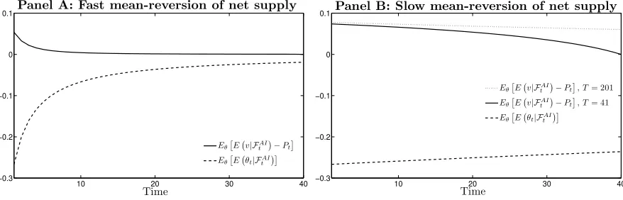
Figure 2: The average expectation of the net supply level and the discrepancy between the average price and the average expectation of the liquidation value. This figure illustrates the relation between the the average expectation of the net supply level and the difference between the average expectation of the liquidation value and the average price when there is mean-reversion of net supply. In both panels,s >0, and so positive values ofEθE v|FAI

t

−Pt

mean that expectations are closer to fundamentals than prices. In panel A the mean-reversion of net supply is fast (ρ= 0), and lots of endogenous information is produced, whereas in panel B the mean-reversion is slow (ρ= 0.9). The rest of the parametrization is common to both panels: T = 41,n= 1,σ_v2= 0.25,Σs= 0,Σ˜s,1= 1, Σs,t˜ = 1010 (1< t≤T−1),σθ2 = 0.1,α= 2,s= 1. The case of a negative underlying signal (s <0)

is the symmetric of the case depicted.

means that, on average, AI’s beliefs about the liquidation value remain biased toward prior beliefs. And this implies that the AI always believes that the contemporaneous net supply level is negative.7

However, the relative weight investors put on prior beliefs when forming posterior beliefs declines as time passes and more prices are observed. Thus, beliefs about the underlying signal and the contemporaneous net supply level become more accurate as time passes, without ever being perfectly accurate. In the 3-period example,

Eθ

E s|Fi

2

=

1

α2_σ4

i,1σ 2

θ + 1

σ2

i,1 +

(1−ρ)2

α2_σ4

i,1σ 2 θ 1 σ2 v + 1

α2_σ4

i,1σ 2

θ + 1

σ2

i,1 +

(1−ρ)2

α2_σ4

i,1σ 2

θ

s >Eθ

E s|Fi

2

Eθ

E θ2|F2i

= −V ar(v|F

i

2)

ασ2

i,1σv2

s >_Eθ

E θ1|F1i

.

The gradual but incomplete convergence of beliefs to the truth implies that the AI always expects short-term trading opportunities to exist, even though the expected profitability of these short-term trading opportunities decreases as time passes. More-over, the riskiness of these short-term trading opportunities increases as the liquidation

7

On average, Eθ(ξt) = v. Since ξt is adapted to Fi

t, we have ξt = E ξt|Fti

and so

EθhEv+pθ,t pt θt|F

i t

i

= v ⇔ EθE θt|Fi t

= pt pθ,t

v−EθE v|Fi

t . If v > 0 and v − EθE v|Fi

t

>0, it then follows thatEθE θt|Fi t

date comes closer, since the chance that a supply shock will not revert completely until the liquidation date increases. Therefore, although average prices are always worse pre-dictors of the fundamental value compared to average expectations, the gap between these two decreases as time passes. This is illustrated in panel A of figure 1 and in figure 2, for the case of a positive underlying signal (the case of a negative underlying signal is the symmetric).

In panel A of figure 2, the mean-reversion of net supply is fast, which generates lots of endogenous information. As a result, there is little uncertainty in the periods close to the liquidation value. In this case, it is the convergence of the average expectation of the net supply level to zero, as opposed to the increased riskiness of short-term trading, the most important factor in the decreased attractiveness of short-term trading as the liquidation date approaches. In panel B the mean-reversion of net supply is low, and the opposite is true: the increase in riskiness is the dominant force. As we can see, the difference between the average expectation and the average price (solid line) converges to zero much faster than it would if the liquidation date took place in a more distant future (dotted line), and much faster than the AI’s expectation of the net supply converges to zero (dashed line).

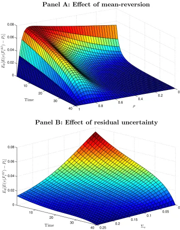
So, we already know that mean-reversion of net supply is crucial to obtain a discrep-ancy between the average price and the average expectation when there is no residual uncertainty. But how do different speeds of mean-reversion and different levels of resid-ual uncertainty affect this result? Figure 3 provides the answer. Panel A shows that an increase in the speed of mean-reversion has a non-monotonic impact in the differ-ence between the average expectation and the average price. This happens because, on the one hand, for a given expectation of the current net supply level, a faster mean-reversion increases the expected profitability of the short-term trading opportunities. But, on the other hand, the faster the mean-reversion, the more endogenous information is produced. The latter means that the expectation of the current net supply level will be closer to zero at all dates, which decreases the expected profitability of the short-term trading. This is specially true in the periods more distant from the initial release of exogenous information, since more endogenous information has been accumulated. The first effect, which tends to increase the divergence between the average expectation and the average price, dominates only whenρis close to 1, otherwise the second effect, which tend to decrease that divergence, dominates.

expec-0 0.2

0.4 0.6

0.8 1

10 20

30 40 0

0.02 0.04 0.06 0.08

ρ

Panel A: Effect of mean-reversion

Time

Eθ

[

E

(

v

|F

A

I

t

)

−

Pt

]

0 0.05 0.1

0.15 0.2

0.25 10

20

30

40 0

0.02 0.04 0.06 0.08

Σs

Panel B: Effect of residual uncertainty

Time

Eθ

[

E

(

v

|F

A

I

t

)

−

Pt

]

Figure 3: Comparative statics on the discrepancy between the average price and the average expectation of the liquidation value when there is mean-reversion of net supply.

This figure shows how the speed of mean-reversion of net supply (panel A) and the level of residual uncertainty (panel B) impacts the difference between the average expectation of the liquidation value and the average price when the underlying signal is positive (the negative case is the symmetric) and there is mean-reversion of net supply. Positive values mean that expectations are closer to fundamentals than prices. In panel Aρ∈[0,1],Σs= 0ands= 1. In panel Bρ= 0.8,Σs∈[0,0.25]andsis adjusted

so that the fundamental value remains unchanged as the level of residual uncertainty changes (higher residual uncertainty requires higher s). The remaining parametrization is common to both panels:

tation and the average price decreases with the level of residual uncertainty.

To sum up, the release of private exogenous information based on an underlying signal that differs from investors’ prior beliefs (s 6= 0) and the mean-reversion of net supply are the two key ingredients to create a discrepancy between the average price and the average expectation of the liquidation value. The former makes the average investor believe that the price movement contemporaneous to the release of exogenous information was partly driven by noise/liquidity demand. And the latter makes the average investor expect liquidity traders to gradually exit the market. This creates an opportunity to profit from liquidity traders on the short-run, which diverts attentions from the long-run. As a consequence, the average price differs from the average expec-tation of the liquidation value: the latter is always closer to the fundamental value than the former.

An alternative way of looking at this is the following. When investors expect to trade in the short-term, they care not only about the final liquidation value, but also about intermediate prices. Since prices reflect the opinions of all other investors about the liquidation value, each investor has to forecast others’ opinions. These opinions reflect both the common prior information (which is public information) and the private signal. As Allen et al. (2006) put it:

“Now suppose that the individual is asked to guess what the average expectation of the asset’s payoff is. Since he knows that others have also observed the same public signal, the public signal is a better predictor of average opinion; he will put more weight on the public signal than on the private signal. Thus if individuals’ willingness to pay for an asset is related to their expectations of the average opinion, then we will tend to have asset prices overweighting public information relative to the private information.”

This over-reliance on public information then causes the average price to deviate more from the fundamental value than the average expectation of the liquidation value.

4.3

Release of Additional Exogenous Information

The second modification to the base case is the release of additional exogenous informa-tion, which I consider here in place of the mean-reversion of net supply. I will analyze a version of the model incorporating these two features simultaneously in the next sub-section. I assume that there are two dates at which exogenous information is released. The generalization to a larger number of information release dates is straightforward. In addition, I assume that the second date of information release is the last trading date (T −1). This is without loss of generality since, as we saw in Section 4.1, when there is no additional exogenous information to be released in the future and no mean-reversion of net supply, the average price and average expectation of the liquidation date coincide at all dates. Therefore, exogenous information is assumed to be released at dates 1 and

T −1.

As we saw previously, investors need to engage in short-term trading for the average price to diverge from the average expectation of the liquidation value. For the former to happen, though, investors need to expect short-term price movements. In this setting, the only thing that can generate predictable short-term price changes is the incoming release of exogenous information. So, let us examine the expected impact of additional exogenous information... on investors’ demands. I will get to prices later on.

Every investor anticipates two effects of the release of additional information: (i) the beliefs about the liquidation value will become more homogeneous which, for a given price, tends to make investors’ demands more homogeneous as well; (ii) beliefs about the liquidation value become more precise, which leads investors to trade more aggressively based on their expectations, thus making their demands more heterogeneous. Therefore, whether the release of additional information makes demands more homogeneous or more heterogeneous, depends on which of these two effects dominate.

Curiously, when there is no residual uncertainty, the two effects exactly offset each other. That is, every investor expects the release of additional exogenous information to have no effect on the demand of every other investor. Investors may expect prices to change though,

E ∆Pt+τ|Fti

=αV ar v|Fi

t+τ−1

−V ar v|Fi t+τ

Xt.

that is,

X_ti = E(v|F

i t)−Pt

αV ar(v|Fi t)

. (10)

Focusing now on our AI, averaging over net supply shocks it follows that, ∀τ

Eθ,i

E ∆Pt+τ|Fti

=αV ar v|FAI

t+τ−1

−V ar v|FiAI

t+τ

Eθ,i(Xt) = 0

and so

Eθ,i

E v|Fi t

=Eθ(Pt).

Therefore, when there is no residual uncertainty, the average price equals the average expectation of the liquidation value at all dates.

When there is residual uncertainty, though, the first effect always dominates the sec-ond, meaning that investors expect demands to become more homogeneous in response to the release of additional exogenous information. This happens because investors receive information about the underlying signal and not about the liquidation value. When there is residual uncertainty, the former is only a noisy signal for the latter. What this means is that, in relative terms, the new information resolves less uncertainty about the liquidation value than it resolves uncertainty about the underlying signal. As a con-sequence, the trading aggressiveness increases less than it would increase if there were no residual uncertainty and the underlying signal coincided with the liquidation value. Hence, the first effect dominates. But the simplest way to illustrate why residual un-certainty leads to more homogeneous demands, is to consider what happens when the incoming exogenous information resolves all uncertainty about the underlying signal. In this case all investors will share the same beliefs. When there is residual uncertainty, the asset remains risky, and so in equilibrium every investor demands the same quan-tity. Obviously, demands become more homogeneous. In contrast, if there is no residual uncertainty, then the asset becomes riskless. This makes investors indifferent between demanding any quantity in equilibrium, and so they can keep their previous demand unchanged and the market still clears.

The latter means that he believes the idiosyncratic error of his signal was positive. That is the AI believes that the majority of investors received less optimistic signals and, in particular, that the average investor his somebody else who has observed a less optimistic signal. Even though there will be some endogenous production of information going on (more on this later), the AI will maintain these qualitative beliefs at all dates until additional exogenous information is released.

Let us start by considering what happens to the average price and average expec-tation at the date immediately before the release of new information, date T −2. As mentioned before, on average the AI believes that the current net supply level is nega-tive. Because he expects demands to become more homogeneous following the release of new information at dateT −1, he expects his own date T −1 demand to decrease and become negative (recall that market equilibrium requires that his demand be zero at dateT −2). Since at dateT −1 we are back to the base case, demands are as in the static model, and given by equation (10). Therefore, if the AI expects to demand a neg-ative quantity, he has to expect a price above his current expectation of the liquidation value, that is,Eθ

E ∆PT|FTAI−2

<0.

Market clearing at date T −2 requires the AI to demand zero. Thus, the short-term demand has to offset the hedging demand that results from the expectation of a negative demand atT−1. The sign of the hedging demand will depend on the precision of the exogenous information released at date T −1. If information is precise enough, the correlation between∆PT−1and∆PT will be positive, resulting in a positive hedging

demand. But hedging demand can also be null or negative if information is not precise enough. Let us consider first the case of negative hedging demand. In this case, the short-term demand has to be positive, which means that Eθ

E ∆PT−1|FTAI−2

> 0. However, under assumption 5, the hedging demand offsets the short-term demand only if Eθ

E ∆PT−1+ ∆PT|FTAI−2

<0, and so we obtain that

Eθ(PT−2)>Eθ

E v|FAI T−2

.

The case of positive or null hedging demand is straightforward. In these cases, market clearing requires a weakly negative short-term demand, which implies that Eθ

E ∆PT−1|FTAI−2

≤0. It is then immediate thatEθ

E ∆PT−1+ ∆PT|FTAI−2

<0 and so Eθ(PT−2) > Eθ

E v|FAI T−2

10 20 30 40 −0.8

−0.6 −0.4 −0.2 0

Panel A: Price discrepancy and expected net supply

Time

Eθ£E¡v|FAI

t ¢

−Pt¤

Eθ£E¡θt|FAI

t ¢¤

10 20 30 40

0.55 0.6 0.65 0.7 0.75

0.8 Panel B: 3 incoming releases of information

Time

Eθ(Pt)

Eθ

£

E¡v|FAI

t ¢¤

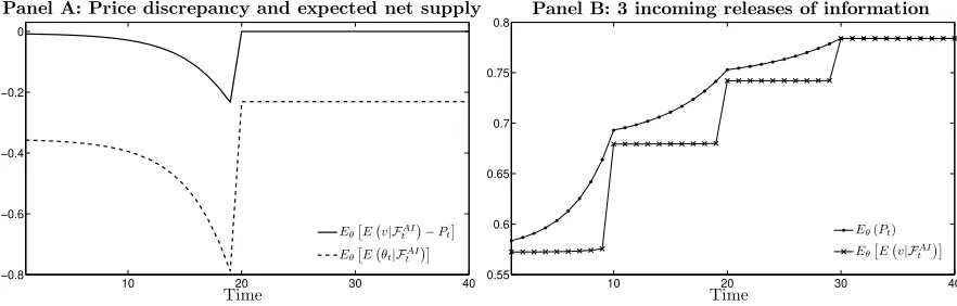
Figure 4: Discrepancy between the average price and the average expectation of the liquidation value. This figure shows how the average expectation of the liquidation value differs from the average price when there is an incoming release of information based on the same underlying signal and the underlying signal is positive (the negative case is the symmetric). Panel A shows the relation between that difference and the average expectation of the net supply level when new information is released at date 20, with Σ˜s,20 = 0.1 and Σ˜s,t = 1010∀t\ {1,20}. Negative values of EθE v|FAI

t

−Ptmean that prices are closer to fundamentals than expectations. Panel B shows that difference when there is more than one incoming release of information, withΣs,˜10= Σ˜s,20= Σs,˜30= 1

andΣ˜s,t= 1010∀t\ {1,10,20,30}. In both panels, the remaining parametrization is the same: T = 41, n= 1,ρ= 1,σ2_v= 0.25,Σs= 0.5,Σ˜s,1= 1,σ2θ= 0.1,α= 2,s= 3.

now believes that the net supply is even more negative than before.8

Therefore, the AI now expects a larger reduction in his demand at dateT −1 than before, which implies that he expects a larger discrepancy between PT−1 and Eθ

E v|FAI T−τ

. And this translates into a bigger difference betweenPT−τ andEθ

E v|FAI T−τ

. Figure 4 provides an illustration. In addition, panel B confirms that, as mentioned in the beginning of this subsection, all the results generalize to the case where there is more than one incoming release of information.

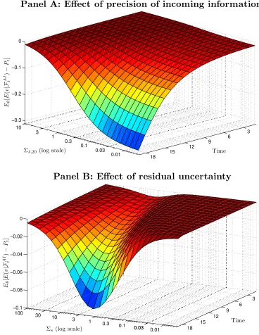
We just saw that the discrepancy between the average expectation and the average price stems from the combination of incoming release of exogenous information and residual uncertainty. The next question is how does that discrepancy change with the precision of incoming information and with the level of residual uncertainty. Obviously, the expected price impact of the incoming information increases with its precision. Thus, unsurprisingly the discrepancy between the average price and the average ex-pectation increases with the precision of the incoming information, as we can see from panel A of figure 5.

In turn, as we can see from panel B, the increase in the level of residual uncertainty has a non-monotonic impact on the difference between the average expectation and the average price. The reason for this is that an increase in the level of residual uncer-tainty produces two effects on the profitability of short-term trading, and thus on the discrepancy between the average price and the average expectation. On the one hand, the higher the level of residual uncertainty, the more homogeneous the demands are expected to become after the release of the new information. As we saw, this tends to increase the expected profitability of short-term trading. But, on the other hand, as the residual uncertainty increases, the relevance of the incoming information decreases, since it resolves a smaller fraction of the overall uncertainty. Therefore, the expected price impact of the new information tends to decrease, which decreases the expected profitability of short-term trading. The first effect dominates only when the residual uncertainty is not too large, reason why initially the discrepancy between the average price and the average expectation increases with the level of residual uncertainty. But then after some point the second effect takes over and this difference starts decreasing with the level of residual uncertainty.

Summing up, the release of additional exogenous information based on the same

8

0.01 0.1

1 3 10

0.3

0.03

3 6 9 12 15 18 −0.3

−0.2 −0.1 0

Time

Panel A: Effect of precision of incoming information

Σs,˜20(log scale)

Eθ

[

E

(

v

|F

A

I

t

)

−

Pt

]

0.01 0.1

1 10

100 30

3

0.3

0.03 0.03

3 6 9 12 15 18 −0.1

−0.08 −0.06 −0.04 −0.02 0

Time

Panel B: Effect of residual uncertainty

Σs(log scale)

Eθ

[

E

(

v

|F

A

I

t

)

−

Pt

]

Figure 5: Comparative statics on the discrepancy between the average price and the average expectation of the liquidation value when there is an incoming release of exoge-nous information. This figure shows how the precision of incoming information (panel A) and the level of residual uncertainty (panel B) impacts the difference between the average expectation of the liquidation value and the average price when the underlying signal is positive (the negative case is the symmetric) and there is an incoming release of exogenous information. Negative values mean that prices are closer to fundamentals than expectations. In panel AΣ˜s,20 ∈[0,10], Σs = 0.5 and s= 3.

I panel B:Σs∈[0,100],Σs,˜20 = 1and sis adjusted adjusted so that the fundamental value remains

underlying signal as previously released private exogenous information, and residual uncertainty, are the two key ingredients to create a discrepancy between the average price and the average expectation, and bring the former closer to the fundamental value than the latter. Together, these two factors lead investors to speculate on the price impact of incoming information, engaging in short-term speculative trading. This diverts attentions from the long-run and allows a divergence in the average price and average expectation of the liquidation value to persist.

As in the case of mean-reversion of net supply (previous subsection), investors care not only about the liquidation value, but also about intermediate prices. For this reason, investors have to forecast the opinions of other investors. But in this case, forecasting the opinions of others does not call for overweighting public information. On the one hand, all investors observed the same public information (the common prior), and a private signal. Although any given investor knows what the public information was, he can only make an inaccurate estimate of what those private signals might have been, hence the tendency to over-rely on public information. But, on the other hand, all investors will observe another private signal related to the private signal already observed. Since the incoming private signal can be forecasted with the previously observed private signal, investors will overweight their private signal when forming their beliefs about others’ beliefs. Therefore, prices will under-rely on public information.

This is what Allen et al. (2006) overlook when they asserted that short-term spec-ulative trading always leads to over-reliance on public information. Even though in their model there is release of exogenous information at all dates, there is no residual uncertainty and net supply mean reverts. This is why they always obtain over-reliance but never under-reliance on public information.

4.4

The General Case: Mean-Reversion of Net Supply and

Re-lease of Additional Exogenous Information

0.01 0.1

1

0.03 0.3

3 10

3 6 9 12 15 18 −0.02

−0.01 0 0.01 0.02

Time

Panel A: Effect of precision of incoming information

Σ˜s,20 (log scale)

Eθ

[

E

(

v

|F

A

I

t

)

−

Pt

]

0.01 0.03

3

0.3

10

1

0.1 3

6 9

12 15

18 0

0.02 0.04 0.06

Σs(log scale)

Panel B: Effect of residual uncertainty

Time

Eθ

[

E

(

v

|F

A

I

t

)

−

Pt

]

residual uncertainty causes under-reliance on public information, their result tells us the conditions in which each of the two effects dominates.

0.85

0.9

0.95

1 3

6 9

12 15

18 −0.15

−0.1 −0.05 0 0.05

ρ

Panel C: Effect of mean-reversion of net supply

Time

Eθ

[

E

(

v

|F

A

I

t

)

−

Pt

]

Figure 6: Comparative statics on the discrepancy between the average price and the average expectation of the liquidation value when there is mean-reversion of net supply and an incoming release of exogenous information. This figure shows how the precision of precision of incoming information (panel A), the level of residual uncertainty (panel B) and the speed of mean-reversion of net supply (panel C) impacts the difference between the average expectation of the liquidation value and the average price when there is an incoming release of exogenous information and mean-reversion of net supply, and the underlying signal is positive (the negative case is the symmetric). In panel AΣ˜s,20∈[0,10], Σs= 0.5 andρ= 0.9. In panel BΣs∈[0,10],Σs,˜20 = 0.2and ρ= 0.9. In

panel Cρ∈ [0.82,1], Σs = 0.25 and Σs,˜20 = 0.2. The remaining parametrization is the same in all

panels: T = 41, n= 1, σ_v2 = 0.25, Σs,˜1= 1, Σs˜i_,t = 1010∀t\ {1,20}, σ2_θ = 0.1, α= 2. In all panels,

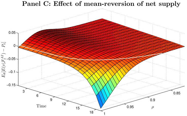
the white line corresponds to the intersection of the surface plot with the plane defined by the average price equal to the average expectation of the liquidation value. Positive (negative) values mean that prices are further away (closer) to fundamentals than expectations.

release of the initial information. This is shown in panel C of figure 1.

Figure 6 shows how changing each of the three relevant parameters, precision of incoming information (Σ˜s,20), level of residual uncertainty (Σs) and speed of

mean-reversion of net supply (ρ), can tilt the balance toward under-reliance or over-reliance on public information.

5

Discrepancy between Average Prices and

Expecta-tions: The Case of Multiple Underlying Signals

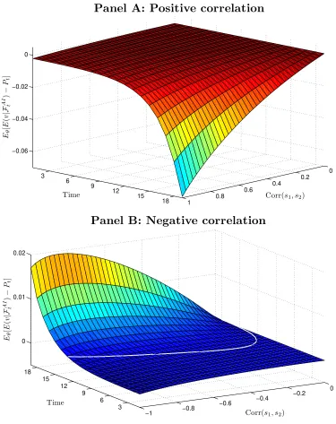
In contrast to the previous section this section, here I consider that different releases of exogenous information are based on different underlying signals. Provided that the two underlying signals are positively correlated, the qualitative results of Section 4.3 remain unchanged, as we can see from panel A of figure 7.

0 0.2 0.4 0.6 0.8 1

3 6

9 12

15 18 0

−0.02

−0.04

−0.06

Corr(s1, s2)

Panel A: Positive correlation

Time Eθ

[

E

(

v

|F

A

I

t

)

−

Pt

]

−1 −0.8

−0.6 −0.4

−0.2 0

3 6 9 12 15 18 0 0.01 0.02

Corr(s1, s2)

Panel B: Negative correlation

Time

Eθ

[

E

(

v

|F

A

I

t

)

−

Pt

]

Figure 7: The correlation between underlying signals and the discrepancy between the average price and the average expectation of the liquidation value. This figures shows how the difference between the average expectation of the liquidation value and the average price changes with the correlation between the signal underlying the past release of information (s1) and

the signal underlying the incoming release of information (s2), when there is no mean-reversion of

net supply. In panel A the correlation ranges from 0 to 1, and in panel B from 0 to -1. In both

panels the parametrization is as follows: T = 41, n= 2, ρ= 1, σ2

v = 0.25, Σs =

0.25 σs1,s2 σs1,s2 0.25

,

Σs,˜1=

1 0 0 110

, Σ˜s,20 =

110 ₀ 0 0.2

, Σ˜s,t=

110 ₀ 0 110

∀t\ {1,20},σ2_θ = 0.1, α= 2,s1 = 1,

s2 = 1. The white line corresponds to the intersection of the surface plot with the plane defined by

reversing later on. This result stems from a different correlation structure between expected price changes and the consequent impact on hedging demands.

In any case, the link between over-(under-)reliance on public information and prices being closer (further away) from fundamentals than expectations is preserved. When correlation is negative prices start by under-relying on public information and then after some point over-rely on public information

Now I switch the attention to how the existence of multiple underlying signals change the results of Section 4.2. As we saw in Section 4.2, when there is mean-reversion of net supply, prices under-rely on public information after the last release of exogenous information, and therefore prices are further away from fundamentals than expectations (see panel A and C of figure 1). However, when there are multiple underlying signals, this is no longer true. Even though prices under-rely on public information after the last information release, they may be either closer of further away from fundamentals than expectations. It all depends on the value of the underlying signals.

Before I proceed, I need to provide the definition of fundamental when there is more than one underlying signal. The date t fundamental value is now the expectation of the liquidation obtained from the direct observation of all underlying signals for which exogenous information was already released by datet. This means that the fundamental value changes whenever exogenous information for a new underlying signal is released for the first time.

From now on, let us focus on the case of two distinct underlying signals. Generalizing from lemma 6, we have that, after the release of the second and last exogenous informa-tion, the fundamental value, average price and average expectation of the liquidation value are given by

F Vt = Kˆs

= a1s1+a2s2

Eθ(Pt) = Kˆs+

ˆ

K−_pˆ_t{Eθ[E(s|Fc

t)]−s}

= F Vt+b1,t{Eθ[E(s1|Ftc)]−s1}+b2,t{Eθ[E(s2|Ftc)]−s2}

Eθ,i

E v|Fti

= Kˆs+ ˆKI2−Γˆt

{Eθ[E(s|Ftc)]−s}

= F Vt+c1,t{Eθ[E(s1|Ftc)]−s1}+c2,t{Eθ[E(s2|Ftc)]−s2}

a function of s2, we find that they will eventually cross with each other at some point. But, for prices to be further away from fundamentals than expectations in all scenarios, the three variables have to cross at the same point. This happens if and only if there is a s2 that solves the following system of equations

 



b1,t{Eθ[E(s1|Ftc)]−s1}+b2,t{Eθ[E(s2|Ftc)]−s2}= 0

c1,t{Eθ[E(s1|Ftc)]−s1}+c2,t{Eθ[E(s2|Ftc)]−s2}= 0

,

that is, we need b1,t

b2,t =

c1,t

c2,t orEθ[E(s1|F

c

t)]−s1 = 0 . However, generically the former

does not hold, even though b1,t > c1,t and b2,t > c2,t (over-reliance on public

informa-tion), and so the system of equations is solved only when both signals coincide with the prior belief on the liquidation value.9

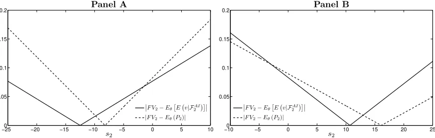
Therefore, if the first underlying signal does not coincide with its unconditional mean, then there are some values of the second underlying signal that bring the average price closer to the fundamental value than the average expectation. In other words over-reliance on public information is no longer a synonym of prices being further away from fundamentals than expectations.

Figure 8 illustrates the situation. In panel A the fundamental value is more sensitive tos2 than the average expectation, and in turn the latter is more sensitive to s2 than the average price. In this case there is a bounded region ofs2values for which prices are closer to fundamentals than expectations. In contrast, in panel B the average expec-tation is more sensitive to s2 than the average price and the fundamental value. Now there is an unbounded region of s2 values for which prices are closer to fundamentals than expectations.

6

Other Implications

The model developed in this paper delivers two other implications worth noting. The first is the apparent leakage of inside information in the periods preceding the release of exogenous information, which we can see from panels B and C of figure 1. Prices appear to be move in anticipation and direction of the new information release. How-ever, we know that in this model prices move in anticipation to the new information, but in the direction of previous information. Investors trade in anticipation to the impact of new information, and in doing so use their information more aggressively, which impounds more of the existing information into prices. Moreover, this is only

9

−250 −20 −15 −10 −5 0 5 10 0.05

0.1 0.15 0.2

s2

Panel A

¯ ¯F V2−Eθ

£

E¡v|FAI

2 ¢¤¯¯

|F V2−Eθ(P2)|

−100 −5 0 5 10 15 20 25

0.05 0.1 0.15

0.2 Panel B

s2

¯ ¯F V2−Eθ

£

E¡v|FAI

2 ¢¤¯¯

|F V2−Eθ(P2)|

Figure 8: Distance of average expectation of the liquidation value and average price to the fundamental value, as a function of the second underlying signal. This plot shows the distance of the average expectation of the liquidation value and of the average price to the fundamental value as a function of the second underlying signal (s2). These distances are computed at the date the

information based on that underlying signal is released. The fundamental value, average expectation and average price are linear functions of s2, and so cross at most once. In panel A, the average

expectation and average price cross at the rightmost intersection of the difference lines, whereas in

panel B they cross at the leftmost intersection. In panel A Σs,˜2 =

110 0 0 0.4

, and in panel B

Σs,˜2=

110 ₀ 0 0.3

. The rest of the parametrization is identical in both panels: T = 4,n= 2,ρ= 0,

σ_v2= 0.25,Σs=

0.25 0 0 0.25

,Σ˜s,1=

1 0 0 110

,Σ˜s,3=

110 0 0 110

,σ_θ2= 0.1, α= 2,s1= 1.

the case when investors have private information about an underlying signal that is positively correlated with that of the incoming information. Therefore, prices can and will sometimes move in the opposite direction of the new information. However, as long as the underlying signal of new and old information are positively correlated, good news tend to be folowed by good news and bad news by bad news. Thus, most of the time the price movement in anticipation to the release of new information is in the right direction, making it look like leakage of inside information.

of Cespa (2002), who finds the opposite relation when the economy is populated by short-term investors.

7

Conclusion

In this paper I show how the existence of short-term trading causes a divergence between the average price and the average expectation of the fundamental value. When investors engage in short-term trading, they care about intermediate prices. This embeds higher-order expectations into prices which cause a discrepancy betw