Munich Personal RePEc Archive
The folk rule through a painting
procedure for minimum cost spanning
tree problems with multiple sources
Bergantiños, Gustavo and Navarro, Adriana
Universidade de Vigo
25 January 2019
Online at
https://mpra.ub.uni-muenchen.de/94312/
The folk rule through a painting procedure for
minimum cost spanning tree problems with multiple
sources
✩G. Berganti˜nos, A. Navarro-Ramos∗
Economics, Society and Territory. Facultad de Economa, Campus Lagoas-Marcosende, s/n, Universidade de Vigo, Vigo, Pontevedra, Spain
Abstract
We consider minimum cost spanning tree problems with multiple sources. We propose a cost allocation rule based on a painting procedure. Agents paint the edges on the paths connecting them to the sources. We prove that the painting rule coincides with the folk rule. Finally, we provide an axiomatic characterization.
Keywords: minimum cost spanning tree problems with multiple sources, painting rule, axiomatic characterization.
1. Introduction
We study situations where a group of agents need services provided by several sources. Agents need to be connected, directly or indirectly, to all sources. Every connection is costly. Situations of this kind are called minimum cost spanning tree problems with multiple sources and are extensions of the classical minimum cost spanning tree problem (where there is a single source).
The first issue addressed is to find the least costly networks connecting all agents with all sources. Obviously, such a network is a tree. It can also be found in polynomial time using the same algorithms as in the classical problem (e.g., Kruskal (1956) and Prim (1957)).
The second issue addressed is how to allocate the cost of the tree obtained among the agents. Several papers have studied this issue in minimum cost span-ning tree problems, but as far as we know only three have considered it in the
✩This work is partially supported by the Spanish Ministerio de Econom´ıa y
Competi-tividad [grant number ECO2014-52616-R]; Xunta de Galicia [grant number GRC 2015/014], Fundaci´on S´eneca de la Regi´on de Murcia [grant number 19320/PI/14]; and Consejo Nacional de Ciencia y Tecnolog´ıa - CONACyT [grant number 438366].
∗Corresponding author
case of multiple sources. Rosenthal (1987) and Kuipers (1997) study a situation slightly different from this paper, whereas Berganti˜nos et al. (2017) study the same situation as we present here. Rosenthal (1987) considers situations where all sources provide the same service and agents want to be connected to at least one of them. He considers a cooperative game and studies the core of that game. Kuipers (1997) considers situations where each source offers a different service and each agent needs to be connected to a subset of the sources. He also considers a cooperative game and seeks to determine under what conditions the core is non-empty. Berganti˜nos et al. (2017) study the same situation as in this paper. They extend different definitions of the folk rule, defined for classical minimum cost spanning tree problems, to the case of multiple sources. They also present some axiomatic characterizations of the folk rule.
In classical minimum cost spanning tree problems the folk rule is one of the most important rules. It has been studied in several papers, including Berganti˜nos and Kar (2010), Berganti˜nos et al. (2010, 2011, 2014), Berganti˜nos and Vidal-Puga (2007, 2009), Branzei et al. (2004), and Tijs et al. (2006).
Our paper is closely related to that of Berganti˜nos et al. (2014). They study a general framework of connection problems involving a single source, which contains classical minimum cost spanning tree problems. They propose a cost allocation rule, called the painting rule because it can be interpreted through a painting story. The idea is the following: start with a treet; for each agent, identify the unique path intfrom that agent to the source. Agents start painting the first edge on that path. Following a protocol, an agent continues painting until all edges on her path have been painted. They also give some axiomatic characterizations of the painting rule. They prove that the painting rule coincides with the folk rule in classical minimal cost spanning tree problem. Thus, they obtain a new way of computing the folk rule and a new axiomatic characterization.
The first objective of this paper is to extend the definition of the painting rule to the case of minimum cost spanning tree problems with multiple sources. The main problem that arises when doing this is that given a tree and an agent, several paths in the tree could connect the agent to a source. In order to avoid this problem, we define a two-phase procedure: In Phase 1, given a treet, we compute a tree t∗ with the same cost as t such that t∗ is also a tree when it
is restricted to the set of sources. Notice that for each agent there is a unique path int∗connecting the agent with the set of all sources. In Phase 2 we apply
the ideas of the painting rule to the treet∗. This extension of the painting rule is not straightforward because it could depend on the treetconsidered initially and the tree t∗ computed in Phase 1, which is not determined solely byt. In
Proposition 2 we prove that for each treetandt∗ considered, the painting rule
always coincide with the folk rule. Thus, the painting rule is independent of the treest andt∗ considered.
are quite standard in the literature and are defined as in the classical minimum cost spanning tree problem. Cost monotonicity says that if the connection cost between two nodes increases, no agent can be better off. Symmetry says that agents with the same connection costs to other nodes must pay the same. Cone-wise additivity says that the rule should be additive on the cost function when it is restricted to cones. The isolated agents property is inspired by the property (also called isolated agents) introduced in Berganti˜nos et al. (2014). Nevertheless, the extension is not so straightforward as with the previous ones. An agent is isolated when all her connection costs are the same and she does not benefit from connecting to the sources through the rest of the agents. If all sources can be connected to one another for free, then an isolated agent should only pay her connection cost to any node. Equal treatment of source costs is a property defined only in the case of multiple sources. It is introduced in Berganti˜nos et al. (2017) and states that if the connection cost between two sources increases then all agents must be affected in the same way.
The paper is organized as follows. Section 2 introduces minimum cost span-ning tree problems with multiple sources. Section 3 introduces the painting rule. Section 4 gives the axiomatic characterization.
2. The minimum cost spanning tree problem with multiple sources
We consider situations where a group of nodes N (called agents) wants to be connected to a set of suppliersM (called sources).
LetN={1, ..., n}be the finite set of agents andM ={a1, ..., am} the finite
set of sources. There is acost matrix C= (cij)i,j∈N∪M overN∪M representing
the cost of the direct link between any pair of nodes, with cji =cij ≥ 0 and
cii = 0, for all i, j ∈N∪M. We denote by CN∪M the set of all cost matrices
overN∪M.
Aminimum cost spanning tree problem with multiple sources(briefly, a prob-lem) is a triple (N, M, C) whereN is the set of agents,M is the set of sources and C ∈ CN∪M is the cost matrix. If c
ij ∈ {0,1}, for all i, j ∈ N ∪M, then
(N, M, C) is called asimple problem.
Anedge is a non-ordered pair (i, j) such thati, j ∈N ∪M. Sometimes we writeij instead of (i, j). Anetwork gis a subset of edges. The cost associated with a networkg is defined as
c(N, M, C, g) = X
(i,j)∈g
cij.
When there are no ambiguities, we writec(g) orc(C, g) instead ofc(N, M, C, g). Given a networkg and any pair of nodesiand j, apath from ito j ing is a sequence of distinct edgesgij ={(ih−1, ih)}qh=1 satisfying that (ih−1, ih)∈g
for allh= 1, ..., q, i=i0 andj=iq. Acycleis a path fromito iwith at least
two edges. A tree is a graph without cycles that connects all the elements of
Two nodesi, j areconnected ing if there exists a path fromito j. We say thatS ⊆N∪M is aconnected component ong if every i, j∈S are connected ingandSis maximal,i.e., for eachT∈N∪M withS(T there existk, l∈T,
k6=l, such thatkandl are not connected ing.
Let (N, M, C) be a simple problem. We denote byg0,C the network induced
by the edges with zero cost. Namely,g0,C={(i, j) :i, j∈N∪M andc ij= 0}.
We say thati, j∈S⊆N∪M are (C, S)-connected ifiand j are connected in
g0,C. We say thatS is aC-component ifS is a connected component on g0,C.
The first issue addressed in the literature is how to find a tree with the lowest associated cost (which is not necessarily unique). This problem is polynomial and the algorithms of Kruskal (1956) and Prim (1957) enable such a tree, which is called minimal tree (mt), to be computed. We denote by m(N, M, C) the cost of anymt in (N, M, C).
Let (N, M, C) be a problem and t a minimal tree in (N, M, C). For each
i, j∈N∪M we denote bytij the unique path intjoiningiandj. Bird (1976)
defines theminimal network associated with the minimal treetas the problem (N, M, Ct), wherect
ij = max(k,l)∈tijckl. It is well known thatC
tis independent
of the chosent. Then, theirreducible problem(N, M, C∗) of (N, M, C) is defined
as the minimal network associated with any minimal tree of (N, M, C). After obtaining a minimal tree, the second issue addressed is how to divide its cost among the agents. A cost allocation rule (briefly, a rule) is a mapping
f that associates a vectorf(N, M, C)∈RN with each problem (N, M, C) such
thatP
i∈Nfi(N, M, C) =m(N, M, C). Thei-th element off(N, M, C) denotes
the payment of agenti∈N.
One of the most popular rules in the classical minimum cost spanning tree problem (mcstp) is the folk rule. Berganti˜nos et al. (2017) extend the definition of the folk rule to the problem with multiple sources and provide several ways to obtain it. One of them is through cone-wise decomposition.
Norde et al. (2004) prove that every classicalmcstpcan be written as a non-negative combination of classical simple problems. What follows is an adapta-tion of this result to our context.
Lemma 1. For each problem(N, M, C), there exists a positive numberm(C)∈ N, a sequence {Cq}m(C)
q=1 of simple cost matrices and a sequence {xq}
m(C)
q=1 of
non-negative real numbers satisfying three conditions:
(1) C=
m(C)
P
q=1 xqCq.
(2) For eachq∈ {1, . . . , m(C)}, there exists a networkgq such thatcq ij = 1if
(i, j)∈gq andcq
ij= 0 otherwise.
(3) Take q ∈ {1, . . . , m(C)} and {i, j, k, l} ⊂ N ∪M. If cij ≤ ckl, then
cqij ≤cqkl.
Let (N, M, C) be a simple problem and P = {S1, ..., Sp} the partition of
Fi(N, M, C) =
|Sk ∈P :Sk∩M 6=∅| −1
|N| , ifS(i, P)∩M 6=∅
1
|S(i, P)|+
|Sk∈P :Sk∩M 6=∅| −1
|N| , otherwise,
whereS(i, P) is the element ofP to whichibelongs to. Then, the folk rule for a general problem (N, M, C) is defined as
F(N, M, C) =
m(C)
X
q=1
xqF(N, M, Cq).
3. The painting procedure
Given a fixed treet, Berganti˜nos et al. (2014) provide an algorithm to define a rule through a painting procedure in the classicalmcstp. They motivate it as follows.
“ In order to illustrate the procedure used to obtain the rule, assume that the nodes represent the houses of the different agents and the edges are the canals which connect them to an irrigation point. These canals need painting and there is only one machine to do this for each one. The machines cannot be moved to another canal and all of them work at the same speed. At every stage, each agent is assigned to an edge while the path from his house to the source has not been completely painted. The canals inthave painters assigned to them if the painting has not been completed. In each step, the agents assigned to an edge which is not completely painted share equally the time the painting machine is in operation. This can be read as their paying the same cost in that segment. At stage 1, each agent is assigned to the first edge in the unique path intfrom his house to the source. At stages, each agent is assigned to the first unpaid edge in this unique path. If all edges in such a path have already been paid for in the previous stages, then this agent has finished his job. The procedure ends when all edges have been paid for completely.”
We seek to apply the procedure described above to the case of multiple sources. The main problem that arises is that with multiple sources, given a tree t and an agent i, several paths in t could connect agent i to a source in
M. Assume that in the treetall sources are directly connected to one another (namelytM, the restriction ofttoM, is also a tree). In this case, there is only
one path int to connect each agent to the nearest source.
Our idea for extending the definition of Berganti˜nos et al. (2014) to the case of multiple sources is the following. First, given a problem (N, M, C) and an
mt tin (N, M, C), we compute a treet∗ in (N, M, C∗) with the same cost ast
such thatt∗
M is also a tree. Second, we divide the cost oft∗\t∗M using the same
procedure as in Berganti˜nos et al. (2014) and the cost of t∗
M is divided equally
We now give an example where we explain the above procedure intuitively. It is presented formally below.
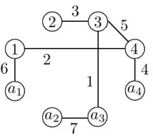
Example 1. Let N = {1,2,3,4}, M = {a1, a2, a3, a4}, c3a3 = 1, c14 = 2,
c23 = 3, c4a4 = 4, c34 = 5, c1a1 = 6, ca2a3 = 7 and cij = 10 otherwise. The
[image:7.612.252.361.204.303.2]minimal treet for this problem is represented in Figure 1.
Figure 1: Minimal tree for (N, M, C).
Notice that the sources are not directly connected to one another. Every agent (except for agent 2) has several paths in t connecting her to a source. For instance, agent1could connect to sourcea1 through path {(1, a1)} or could connect to sourcea4 through path{(1,4),(4, a4)}.
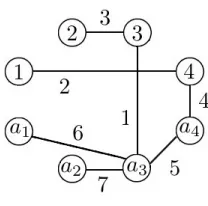
We now construct the tree t∗. We first connect sources a1 and a31. We
remove fromt the most expensive edge on the unique path in t joining a1 and
a3, which is edge (1, a1). We add to t the edge (a1, a3) and we change its cost from 10 to 6 (the cost of edge(1, a1)).
We now connect sources a3 anda4. We remove fromt the most expensive edge on the unique path int joininga3 anda4, which is edge (3,4). We add to
tthe edge (a3, a4)and we change its cost from 10 to 5 (the cost of edge(3,4)). Figure 2 shows the modified tree.
In this tree, each agent has a unique path to the set of sources. The path for agent 1 is{(1,4),(4, a4)}, for agent 2 it is {(2,3),(3, a3)}, for agent 3 it is
{(3, a3)} and for agent 4 it is {(4, a4)}. Then, the original idea of the painting procedure can be applied.
Stage 1. Agent 1 selects edge (1,4), agent 2 selects (2,3), agent 3 selects (3, a3), and agent4 selects(4, a4). Thus, agent3paints edge (3, a3)completely and agents 1, 2 and 4 paint one unit of their edges. Thus, agent 3 is already connected to sourcea3 and she is removed from the procedure.
Stage 2. Agents1, 2 and 4 select the same edges as in Stage 1. Edge(1,4) is completely painted by agent 1. One more unit of edges (2,3) and (4, a4) is painted by agent2 and4, respectively.
1
Figure 2: Alternative tree.
Stage 3. Agent 2 keeps selecting edge (2,3) and agents1 and4 select edge (4, a4). Agent 2 paints one unit of edge (2,3). Agents 1 and4 paint 1
2 of edge
(4, a4). Thus, edge(2,3)is completely painted and agent2is therefore connected to sourcea3 (through agent3) and she is removed from the procedure.
Stage 4. Agents1 and 4 keep selecting edge(4, a4). Each agent paints 12 of edge (4, a4), which is now completely painted. Then, both agents are connected to sourcea4 and removed from the procedure.
[image:8.612.141.528.407.533.2]Stage 5. The edges connecting the sources ((a1, a3), (a2, a3) and (a3, a4)) are painted by all agents.
Table 1 summarizes this procedure.
Agent→ Agent 1 Agent 2 Agent 3 Agent 4
Stage↓ Edge Amount Edge Amount Edge Amount Edge Amount Stage 1 (1,4) 1 (2,3) 1 (3, a3) 1 (4, a4) 1
Stage 2 (1,4) 1 (2,3) 1 (4, a4) 1
Stage 3 (4, a4) 12 (2,3) 1 (4, a4) 12
Stage 4 (4, a4) 12 (4, a4) 12
Stage 5 t∗
M 6+7+54 t
∗
M 6+7+54 t
∗
M 6+7+54 t
∗
M 6+7+54
Total 15
2
15 2
11 2
15 2
Table 1: Summary of the painting procedure.
We now formally introduce the procedure explained in Example 1. We con-sider a two-phase procedure. In the first phase, given anymt t, we construct a treet∗ with the same cost astand where all the sources are connected to one
another. In the second phase we apply the painting procedure as in Berganti˜nos et al. (2014).
Phase 1: Constructing the tree
components induced bytM.
We consider an algorithm to construct a minimal tree t∗ of the irreducible
problem (N, M, C∗).
We start witht0=t. Assume that stageβ is defined, for allβ ≤δ−1.
Stageδ: We have two cases,
• P(tδM−1) ={M}. The algorithm ends andt∗=tδ−1.
• P(tδ−1
M )6={M}. We define
E(tδ−1) ={(ih−1, ih)}qh=1
as the unique path from Sδ
r=1Sr to Sδ+1 in tδ−1, with i0 ∈ Sδr=1Sr,
iq ∈Sδ+1,i1∈/Sδr=1Sr andiq−1∈/ Sδ+1.
Let (i, j) be the most expensive edge inE(tδ−1) (if there are several edges,
then select just one). Namely,
cij = max
(k,l)∈E(tδ−1){ckl}.
We now define,
tδ=tδ−1\(i, j)∪(i0, iq).
This process is completed in a finite number of stages (exactly at m(t)−1 stages and 1 ≤ m(t) ≤ m). The tree t∗ is a mt for (N, M, C∗). Besides
c(C∗, t∗) =c(C, t) andt∗
M is also a tree.
Notice that given a tree t, several trees t∗ could be obtained through this
procedure.
We now formally apply Phase 1 to Example 1. We start with
t0=t={(1, a1),(1,4),(4, a4),(2,3),(3, a3),(3,4),(a2, a3)}.
Stage 1:
• P(t0
M) ={{a1},{a2, a3},{a4}}. Then
E(t0) ={(a1,1),(1,4),(4,3),(3, a3)}.
The most expensive edge inE(t0) is (1, a1). Thus
t1={(a1, a3),(1,4),(4, a4),(2,3),(3, a3),(3,4),(a2, a3)}.
Stage 2:
• P(t1
M) ={{a1, a2, a3},{a4}}. Then
E(t1) ={(a3,3),(3,4),(4, a4)}.
The most expensive edge inE(t1) is (3,4). Thus
Stage 3:
• P(t2
M) ={{a1, a2, a3, a4}}. Then the algorithm ends andt∗=t2.
We know formally define the second phase of our procedure. This phase is obtained by applying the same ideas as in the painting procedure of Berganti˜nos et al. (2014).
Phase 2: Painting the tree.
Let t∗ be an mt in (N, N, C∗) satisfying that t∗
M is a tree over M and
c(N, M, C∗, t∗) =m(N, M, C). By Phase 1 we know that such tree exists. We
take
• e0
i (C, t∗) = ∅for all i ∈N. In general, eδi(C, t∗) denotes the edge of t∗
assigned to agent i at stageδ. Agenti will pay part of the cost of this edge.
• c0(C, t∗) = 0 andcδ(C, t∗) represents the part of the cost of each edge that
it is paid at stageδ.
• p0
i(C, t∗) = 0 for alli ∈N. In general, pδi(C, t∗) is the cost that agent i
pays at stageδ.
• E0(C, t∗) = t∗\t∗
M and Eδ(C, t∗) is the set of unpaid edges oft∗\t∗M at
stageδ.
When no confusion arises we will writeeδ
i,eδi(C) oreδi(t∗) instead ofeδi(C, t∗).
We will do the same withcδ(C, t∗),pδ
i(C, t∗) andEδ(C, t∗). Assume that stage
β is defined, for allβ ≤δ−1. Stageδ:
• For each i ∈ N, leteδ
i be the first edge in the unique path in t∗ from i
to M belonging to Eδ−1. If all edges in such path are not inEδ−1, take eδ
i =∅.
• For each (i, j)∈Eδ−1 we define
Nδ
ij={k∈N :eδk = (i, j)}
and
cδ = min
(
cij− δ−1
X
r=0
cr: (i, j)∈Eδ−1
)
.
• For eachi∈N, we define
pδi =
cδ
N
δ eδ
i
, ifeδ i 6=∅
• We define
Eδ =
(
(i, j)∈Eδ−1:
δ
X
r=0
cr< cij
)
.
This procedure ends when we find a stage γ(C, t∗) (γ(C), γ(t∗) orγ when
no confusion arises) such that Eγ = ∅. Since E0 = t∗\t∗
M, Eδ+1 ⊂ Eδ and
Eδ+16=Eδ,γis finite.
Stage γ+ 1. The cost of all edges ont∗
M,c(t∗M) =
P
(i,j)∈t∗
Mc
∗
ij, is divided
equally among all agents. Then,
pγi+1=c(t
∗
M)
|N| .
For each problem (N, M, C), each mt t, and each i ∈ N, we define the panting rulefiP,t as
fiP,t(N, M, C) =
γ+1
X
δ=1 pδ
i(C, t
∗).
Note that this definition depends on treest andt∗ considered.
We now formally apply Phase 2 to Example 1. We start with:
• e0
1,e02, e03,e04=∅.
• c0= 0.
• p0
1,p02,p03,p04= 0.
• E0={(1,4),(4, a4),(2,3),(3, a3)}.
Stage1:
• e1
1= (1,4),e12= (2,3), e13= (3, a3) ande14= (4, a4).
• N1
14={1},N231 ={2},N31a3={3} andN
1
4a4 ={4}.
• c1= min{c14, c23, c3
a3, c4a4}= min{2,3,1,4}= 1.
• p1
1,p12,p13,p14= 1.
• E1={(1,4),(4, a4),(2,3)}.
Stage2:
• e2
1= (1,4),e22= (2,3), e23=∅ande24= (4, a4).
• N2
14={1},N232 ={2}andN42a4={4}.
• c2= min{c14−1, c23−1, c4
a4−1}= min{2−1,3−1,4−1}= 1.
• p2
• E2={(2,3),(4, a4)}.
Stage3:
• e3
1= (4, a4),e32= (2,3),e33=∅ande34= (4, a4).
• N233 ={2}andN43a4={1,4}.
• c3= min{c23−2, c4
a4−2}= min{3−2,4−2}= 1.
• p3
1= 12,p32= 1, p33= 0 andp34=12.
• E3={(4, a4)}.
Stage4:
• e4
1= (4, a4),e42=∅,e43=∅ande44= (4, a4).
• N4
4a4 ={1,4}.
• c4= min{c4
a4−3}= min{4−3}= 1.
• p4 1= 12,p
4
2= 0, p43= 0 andp44=12.
• E4=∅. Thus,γ= 4.
Stage5: For eachi∈N,
p5i =
c(t∗
M)
4 =
18 4 =
9 2. Then,
f1P(N, M, C) = 1 + 1 +
1 2 +
1 2 +
9 2 =
15 2 ,
f2P(N, M, C) = 1 + 1 + 1 + 0 +
9 2 =
15 2 ,
f3P(N, M, C) = 1 + 0 + 0 + 0 +
9 2 =
11 2 ,
f4P(N, M, C) = 1 + 1 +
1 2 +
1 2 +
9 2 =
15 2 .
We now show that the solution does not actually depend on the minimal treet considered initially and the treet∗ defined in Phase 1. To that end, we
introduce two propositions.
Proposition 1. Let(N, M, C)and(N, M, C′)be two mcstp with multiple sources
satisfying that there is an orderσover the set of edges ofN∪M such that for alli, j, k, l∈N∪M satisfying thatσ(i, j)< σ(k, l), thencij ≤ckl andc′ij≤c′kl.
Lett be a minimal tree inC,C′, andC+C′. Then,
Proof. Applying Phase 1 to t, we can obtain a common mt t∗ for (N, M, C∗),
(N, M, C′∗) and (N, M, C∗+C′∗).
We now compute Phase 2. First, consider the case when for all i, j, k, l ∈
N ∪M satisfying that σ(i, j) < σ(k, l), then cij < ckl and c′ij < c′kl. Thus
cij +c′ij < ckl+c′kl. For all i ∈ N, let iM ∈ N ∪M denote the immediate
successor ofiin the unique path fromitoM in t∗. Without loss of generality,
we assume thatciiM < cjjM wheni < j, for alli, j∈N. Then,
Stage 1:
• ∀i∈N,e1
i(C) =e1i(C′) =e1i(C+C′) = (i, iM).
• ∀i∈N,N1
iiM(C) =Nii1M(C′) =Nii1M(C+C′) ={i}.
• c1(C) = min
i∈N{ciiM}=c11M,
c1(C′) = min
i∈N{c
′
iiM}=c′11M and
c1(C+C′) = min
i∈N{ciiM+c
′
iiM}=c11M+c′11M.
• ∀i∈N,p1
i(C) =c11M,p1i(C′) =c′
11M andp1i(C+C′) =c11M+c′
11M.
• E1(C) =E1(C′) =E1(C+C′) ={(i, iM)}|M| i=2.
Then, for alli∈N,p1
i(C+C′) =p1i(C) +p1i(C′).
Stage 2:
• ∀i∈N\1,e2
i(C) =e1i(C),e2i(C′) =e1i(C′) ande2i(C+C′) =e1i(C+C′).
If 1M ∈ M then e2
i(C) = e2i(C′) = ei2(C+C′) = ∅. If 1M ∈/ M then
e2
i(C) =e2i(C′) =ei2(C+C′) =e11M(C).
Then,∀i∈N,e2
i(C) =e2i(C′) =e2i(C+C′).
• N2
iiM(C) =Nii2M(C′) =Nii2M(C+C′), for alli∈N\{1}.
• c2(C) = min
i∈N\{1}{cii
M−c1(C)}=c22M−c11M,
c2(C′) = min
i∈N\{1}{c ′
iiM−c1(C′)}=c′22M−c′11M and
c2(C+C′) = min
i∈N\{1}{cii
M+c′iiM−c1(C+C′)}=c22M+c′22M−(c11M+
c′11M).
• ∀i∈N,p2
i(C) =
c22M−c11M
|N2
e2 i(C)|
, p2
i(C′) =
c′
22M −c′11M
|N2
e2 i(C
′)| and
p2
i(C+C′) =
c22M+c′22M −(c11M+c′11M)
|N2
e2 i(C+C
′)| .
• E2(C) =E2(C′) =E2(C+C′) ={(i, iM)}|M|
i=2.
Then∀i∈N, p2
Repeating this argument, we can prove thatγ(C) =γ(C′) =γ(C+C′) and
that for each stageδ= 1, ..., γ and for everyi∈N, we have thatpγi(C+C′) =
pγi(C) +pγi(C′). Besides, for everyi∈N,pγ+1
i (C) =
c(t∗
M)
|N| ,p
γ+1
i (C′) =
c′(t∗
M)
|N|
andpγi+1(C+C′) =c(t∗M) +c′(t∗M)
|N| . Thus,
fP,t(N, M, C+C′) =fP,t(N, M, C) +fP,t(N, M, C′).
Now, consider the general case when, ifσ(i, j)< σ(k, l), thencij ≤ckl and
c′ij ≤c′kl. LetCεandC′ε be two cost functions such that:
• For eachi, j∈N∪M,cij−ε≤cεij≤cij+εandc′ij−ε≤cij′ε ≤c′ij+ε
• Ifσ(i, j)< σ(k, l) thencε
ij < cεkl andc′ijε < c′klε.
• tis a minimal tree inCε, C′ε, andCε+C′ε.
Notice that Cε and C′ε satisfy the condition in the first case studied. So,
fP,t(N, M, Cε+C′ε) =fP,t(N, M, Cε) +fP,t(N, M, C′ε).
Finally, taking into account the definition of the rule fP,t, we have that
limε→0fP,t(N, M, Cε) =fP,t(N, M, C), limε→0fP,t(N, M, C′ε) =fP,t(N, M, C′)
and limε→0fP,t(N, M, Cε+C′ε) =fP,t(N, M, C+C′). Thus,
fP,t(N, M, C+C′) =fP,t(N, M, C) +fP,t(N, M, C′).
We now prove that for each problem (N, M, C) and every minimal treetthe painting rule associated witht coincides with the folk rule. Thus, the painting rule is well defined and is independent of the minimal tree t and the tree t∗
computed in Phase 1.
Proposition 2. For every problem (N, M, C) and every minimal tree t for (N, M, C),
fP,t(N, M, C) =F(N, M, C).
Proof. By Lemma 1, we know thatC=
m(C)
P
q=1
xqCqwhere for eachq, (N, M, Cq)
is a simple problem. Besides t is a minimal tree for each (N, M, Cq). By
Proposition 1 and the definition of the folk ruleF, it is enough to prove that
fP,t(N, M, Cq) =F(N, M, Cq) when (N, M, Cq) is a simple problem andt is a
minimal tree in (N, M, Cq).
Lett∗ be a tree obtained on Phase 1. For alli∈N, letiM ∈N∪M denote
the immediate successor of i in the unique path from i to M in t∗. Now, we
apply the procedure of Phase 2: Stage 1: Takei∈N.
• ∀i∈N,e1
i(Cq, t∗) = (i, iM).
• ∀i∈N,N1
Let P = {S1, ..., Sp} be the partition of N ∪M in Cq-components. We
consider several cases:
Case 1: S(i, P)∩M 6=∅, for alli∈N. Then,
• c1(Cq, t∗) = 0. • ∀i∈N,p1
i(Cq, t∗) = 0.
• E1(Cq, t∗) =∅.
Then,γ= 1 and∀i∈N,
p2i(Cq, t∗) =
|Sk :Sk∩M 6=∅| −1
|N| .
Thus,∀i∈N,
fiP,t(N, M, Cq) =
|Sk:Sk∩M 6=∅| −1
|N| =F(N, M, C
q).
Case 2: |S(i, P)|= 1, for alli∈N. ThenS(i, P)∩M =∅,∀i∈N. Now
• c1(Cq, t∗) = 1.
• ∀i∈N,p1
i(Cq, t∗) = 1 =
1
|S(i, P)|.
• E1(Cq, t∗) =∅.
As in the first case,γ= 1 and∀i∈N
p2i(Cq, t∗) = |Sk :Sk∩M 6=∅| −1
|N| .
Therefore
fiP,t(N, M, Cq) = 1
|S(i, P)|+
|Sk :Sk∩M 6=∅| −1
|N| =F(N, M, C
q).
Case 3: Otherwise.
• c1(Cq, t∗) = 0. • ∀i∈N,p1
i(Cq, t∗) = 0.
• E1(Cq, t∗) ={(i, iM)∈E0:cq
iiM = 1} 6=∅.
Stage 2:
• Leti∈N. IfS(i, P)∩M 6=∅, then e2
i(Cq, t∗) =∅. IfS(i, P)∩M =∅,
there exists a uniquej∈S(i, P) such that (j, jM)∈E1. Thuse2
i(Cq, t∗) =
• N2
e2 i(C
q, t∗) =S(i, P).
• c2(Cq, t∗) = 1. • For eachi∈N,
p2i(Cq, t∗) =
0, ifS(i, P)∩M 6=∅
1
|S(i, P)|, otherwise.
• E2(Cq, t∗) =∅.
In this case,γ= 2 and ∀i∈N
p3i(Cq, t∗) =
|Sk :Sk∩M 6=∅| −1
|N| .
Then,
fiP,t(N, M, Cq) =
|Sk :Sk∩M 6=∅| −1
|N| , ifS(i, P)∩M 6=∅
1
|S(i, P)| +
|Sk:Sk∩M 6=∅| −1
|N| , otherwise.
Therefore,fiP,t(N, M, Cq) =Fi(N, M, Cq), for alli∈N.
Since the rule coincides with the folk rule, which does not depend on the treetchosen, the rule can be denoted byfP instead offP,t.
Berganti˜nos et al. (2017) extend the folk rule formcstpwith multiple sources using four approaches: As the Shapley value of the irreducible game (Berganti˜nos and Vidal-Puga (2007)), as an obligation rule (Tijs et al. (2006) and Berganti˜nos and Kar (2010)), as a partition rule (Berganti˜nos et al. (2010, 2011)), and through a cone-wise decomposition (Branzei et al. (2004) and Berganti˜nos and Vidal-Puga (2009)). Thus, the painting rule is a new way of calculating the extension of the folk rule to this context. The main advantage of this approach is that it makes it very clear that the allocation of an agent given by the folk rule depends only on her path to the sources and the connection cost between them in the irreducible problem.
4. An axiomatic characterization
adding a new one called equal treatment of source costs. The definition of the properties of cost monotonicity, symmetry, and cone-wise additivity in the case of multiple sources is the same as in the classical case. The definition of isolated agents is not straightforward. Equal treatment of source costs is a property defined only in the case of multiple sources.
A rulef formcstp with multiple sources satisfies:
Cone-wise additivity (CA). Let (N, M, C) and (N, M, C′) be two mcstp with multiple sources satisfying that there is an order σ over the set of edges of
N∪M such that for all i, j, k, l∈N∪M satisfying thatσ(i, j)< σ(k, l), then
cij ≤ckl andc′ij≤c′kl. Thus,
f(N, M, C+C′) =f(N, M, C) +f(N, M, C′).
CA says that the rule should be additive on the cost functionC when re-stricted to cones.
Cost monotonicity (CM). For all (N, M, C) and (N, M, C′) such that C ≤C′,
then
f(N, M, C)≤f(N, M, C′).
CM says that if a certain number of connection costs increase and the rest (if any) remain the same, no agent should end up better off.
Symmetry (SYM). For all (N, M, C) and all i, j ∈ N such that cik = cjk,
∀k∈(N∪M)\{i, j}, then
fi(N, M, C) =fj(N, M, C).
If two agents are symmetrical with respect to their connection costs,SY M
says that they should pay the same.
The next property is inspired by the isolated agents property introduced in Berganti˜nos et al. (2014) for source connection problems.
An agent i∈N is calledisolated in a problem (N, M, C) ifcij =x, for all
j∈(N∪M)\{i}andcjk≤x, for allj, k∈(N∪M)\{i}. Notice that if agenti
is isolated, then agentidoes not benefit from connecting to the sources through agents inN\{i}.
Isolated agents (IA). For all (N, M, C) such that for allk, l∈M, there is a path fromktol,gkl, such thatc(gkl) = 0,
fi(N, M, C) =x,
for every isolated agenti∈N.
If there is a way of connecting all sources to one another for free (not nec-essarily directly), an isolated agent should only pay her connection cost to any node.
Equal treatment of sources costs (ETSC). For each pair of problems (N, M, C) and (N, M, C′) such that there existk, l ∈ M, k 6=l, such thatc
kl < c′kl and
cij =c′ij otherwise, then for eachi, j∈N
This property was introduced in Berganti˜nos et al. (2017). It says that if the cost between two sources increases, then all agents should be affected in the same way.
In the next theorem, we present the characterization of the painting rule.
Theorem 1. The painting rulefP is the unique rule satisfying CA, CM, SYM,
IA and ETSC.
Proof. First we prove that the painting rule satisfies the five properties. Berganti˜nos et al. (2017) proved that the folk rule satisfies CA CM, SYM and ETSC. By Proposition 2,fP satisfiesCA CM, SYM andETSC.
We now prove that fP satisfies IA. Let i ∈ N be an isolated agent for a
problem (N, M, C). Let t be a minimal tree for (N, M, C). We can taket in such a way that no agent inN\{i} is connected to any source through agenti. Namely, for eachj∈N\{i}and eachk∈M,i /∈tjk.
Since there is a path at cost zero to join together every two sources, the tree obtained in Phase 1,t∗, is such thatc(t∗
M) = 0.
We now apply Phase 2. Since no agent is connected to the source through agent i and cik = x ≥cjk, ∀j, k ∈ (N ∪M)\{i}, we have that, for eachδ =
1, ..., γ, eδ
i = (i, iM) andeδj 6= (i, iM), for allj∈N\{i}.
Then,
fP
i (N, M, C) =ciiM+
c(t∗
M)
|N| =x+ 0 =x.
Thus,fP satisfiesIA.
We now prove the uniqueness. Let f be a rule satisfying the properties of Theorem 1. ByCA, it is enough to prove thatf =fP in simple problems.
Let (N, M, C) be a simple problem and P = {S1, ..., Sp} the set of C
-components. Consider the next cost function:
c′ij =
(
cij, if{i, j} ∩N 6=∅
0, otherwise.
We have a simple problem (N, M, C′) such that all sources are connected to
one another at cost zero andC≥C′.
For eachSk ∈P such thatSk∩M =∅, we define a pair of cost function as
follows:
ck ij=
(
1, if{i, j} ∩Sk 6=∅
0, otherwise
and
c′k ij =
(
c′
ij, if{i, j} ∩Sk 6=∅
We first analyze how f works on (N, M, Ck) and (N, M, C′k). Let S k ∈P
withSk∩M =∅and i∈N.
• On (N, M, Ck). Ifi∈S
k,iis an isolated agent. ByIA,fi(N, M, Ck) = 1,
for alli∈Sk. Besides,m(N, M, Ck) =|Sk|. Since all agents inN\Sk are
symmetric,fi(N, M, Ck) = 0, for alli /∈Sk. This is,
fi(N, M, Ck) =
(
1, ifi∈Sk
0, otherwise.
• On (N, M, C′k). We have thatC′k≤Ck. Ifi /∈S
k, byCM,fi(N, M, C′k)≤
fi(N, M, Ck) = 0. It is straightforward to see that if a rule satisfiesCM
and SYM, then it should be non-negative. Then, fi(N, M, Ck) = 0 if
i /∈Sk. All agents onSk are symmetric andm(N, M, C′k) = 1. Thus,
fi(N, M, C′k) =
1
|Sk|
, ifi∈Sk
0, otherwise.
Takei∈N and letS(i, P) denote theC-component to whichibelongs. We consider two cases.
• S(i, P)∩M =∅. SinceC′≥C′k andCM,
fi(N, M, C′)≥fi(N, M, C′k) =
1
|S(i, P)|.
• S(i, P)∩M 6=∅. Since a rule satisfying CM and SYM should be non-negative
fi(N, M, C′)≥0.
Taking into account thatm(N, M, C′) =|Sk ∈P :Sk∩M =∅|and
X
i∈N
fi(N, M, C′)≥
X
i∈N|S(i,P)∩M=∅
1
|S(i, P)| =|Sk∈P :Sk∩M =∅|,
we conclude that
fi(N, M, C′) =
1
|S(i, P)|, ifS(i, P)∩M =∅
0, otherwise.
Finally, notice that the cost functions C and C′ are as the definition of
ETSC. Then, for alli, j∈N,
Fixi∈N,
|N|[fi(N, M, C)−fi(N, M, C′)] =
X
j∈N
[fj(N, M, C)−fj(N, M, C′)]
=X
j∈N
fj(N, M, C)−
X
j∈N
fj(N, M, C′)
=|P| −1−(|P| − |Sk∈P :Sk∩M 6=∅|)
=|Sk ∈P :Sk∩M 6=∅| −1.
Thus,
fi(N, M, C) =
|Sk∈P :Sk∩M 6=∅| −1
|N| +fi(N, M, C ′)
=
|Sk ∈P :Sk∩M 6=∅| −1
|N| +
1
|S(i, P)|, ifS(i, P)∩M =∅ |Sk ∈P :Sk∩M 6=∅| −1
|N| , otherwise.
Therefore, f(N, M, C) = F(N, M, C). By Proposition 2, f(N, M, C) =
fP(N, M, N).
Next we prove that all properties are needed in the previous characterization. CA is independent of the other properties. Consider the rule fe defined
in Berganti˜nos et al. (2017) when they prove that CA is independent of the properties they use in Theorem 2. fe satisfies all properties butCA.
CM is independent of the other properties. Given a problem (N, M, C), let
t be amt of (N, M, C) andt∗ a mt of (N, M, C∗) obtained through Phase 1.
We now consider the following classical mcstp (N0, C), where c0i = max{c∗kl :
(k, l)∈t∗ij for somej ∈M andk, l∈N} andcij =c∗ij, for alli, j∈N.
For a classical problem with a singlemt, Bird (1976) proposed a rule called the Bird rule. This rule is obtained by requiring each agent to pay the total cost of the first edge in her unique path to the source. Dutta and Kar (2004) extended the Bird rule when there is more than onemt (an extension we denote asB). This rule is the average of the allocations given by the Bird rule on all the minimal trees associated with Prim’s algorithm.
We now extend it to our setting in the following way:
fB(N, M, C) =B(N0, C) +c(t
∗
M)
|N| .
fB satisfies all properties butCM.
SYM is independent of the other properties. For each problem (N, M, C) and eachδ= 1, ..., n+m−1, let (iδ, jδ) denote the edge selected by Kruskal’s
algorithm until stageδ(included). BesidesP(gδ) denotes the partition ofN∪M
in connected components induced bygδ.
Given a partitionP we define the functionαas
αi(P) =
ifS(i, P)∩M =∅ |Sk∈P :Sk∩M 6=∅| −1
|N| + 1, andi≤j,∀j∈S(i, P)
|Sk∈P :Sk∩M 6=∅| −1
|N| , otherwise,
Thus we define the rulefα such that for each problem (N, M, C) and each
i∈N,
fiα(N, M, C) = n+m−1
X
δ=1
ciδjδ[αi(P(gδ−1))−αi(P(gδ))].
fαsatisfies all properties butSYM.
IA is independent of the other properties. Let E be the rule in which the cost of the minimal tree is divided equally among all agents. Namely, for each problem (N, M, C) and eachi∈N,
Ei(N, M, C) =
m(N, M, C)
|N| .
This rule satisfies all properties butIA.
ETSC is independent of the other properties. Let (N, M, C) be a problem. If N = {1,2} and M = {a1, a2}, let us define the sets N′ = {1,2, a2} and
M′={a1}. Then, for every i∈N, we define the rule
fi(N, M, C) =
fP
i (N′, M′, C) +
fP a2(N
′, M′, C)
2 , ifN ={1,2}andM ={a1, a2}
fP
i (N, M, C), otherwise.
This rule satisfies all properties butETSC.
We end this paper by mentioning other properties mey by the rule. These properties are introduced in Berganti˜nos et al. (2017).
Independence of irrelevant trees (IIT). For each (N, M, C) and (N, M, C′), if
they have a common minimal treetsuch that cij =c′ij for each (i, j)∈t, then
f(N, M, C) =f(N, M, C′).
This property requires the cost allocation chosen by a rule to depend only on the edges that belong to a minimal tree.
Core selection (CS). For each (N, M, C) and eachS⊆N,P
i∈Sfi(N, M, C)≤
m(S, M, C).
CS implies that no coalition of agents would be better off by constructing their own minimal tree.
Separability (SEP). For each (N, M, C) and each S ⊆ N, if m(N, M, C) =
fi(N, M, C) =
(
fi(S, M, C), ifi∈S,
fi(N\S, M, C), ifi∈N\S.
Two subsets of agents,SandN\Scan be connected to all the sources either separately or jointly. This property implies that if the minimal costs in two situations are the same, agents will pay the same in both circumstances. Population monotonicity (PM). For each (N, M, C), eachS ⊂T ⊆N and each
i∈S,fi(S, M, C)≥fi(T, M, C).
If new agents join the problem, then no agent in the original problem should be worse off.
These properties are not completely independent. The following proposition summarizes the relations between the properties seen in this paper.
Proposition 3. (i) CM implies IIT. (ii) CS implies AI.
(iii) SEP implies AI.
(iv) PM implies SEP, CS and IA.
Proof. (i) It appears in Berganti˜nos et al. (2017).
(ii) It is easy to see that CS implies IA noticing that, if i ∈ N is an isolated agent in (N, M, C), then m(N, M, C) = m(N\{i}, M, C) +x. Since
P
j∈N\{i}fj(N, M, C) ≤m(N\{i}, M, C) and fi(N, M, C) ≤x, we have that
fi(N, M, C) =x.
(iii) It is similar to Case (ii).
(iv) Berganti˜nos et al. (2017) prove thatPM impliesSEP andCS. By (ii), PM also impliesIA.
Berganti˜nos et al. (2017) also provide two characterizations of the folk rule in minimum cost spanning tree problems with multiple sources. As in Theorem 1, they useCA, SYM, and ETSC. In both cases they also use IIT and com-plete one characterization with CS and the other with SEP. Thus, the three characterizations are unrelated. Namely, no characterization is a consequence of another.
Apart from this, the proof of uniqueness in the characterization of this paper and the proof of uniqueness in the characterizations of Berganti˜nos et al. (2017) are also unrelated. In all three cases the first step is the same. ByCA we can consider only simple games. But now the arguments are completely different. In this paper we consider the problemsC′,C′k, andCk and depending on how
References
Berganti˜nos, G., Chun, Y., Lee, E., Lorenzo, L., 2017. The folk rule for minimum cost spanning tree problems with multiple sources. Mimeo, Universidade de Vigo.
Berganti˜nos, G., G´omez-R´ua, M., Llorca, N., Pulido, M., S´anchez-Soriano, J., 2014. A new rule for source connection problems. European Journal of Oper-ational Research 234 (3), 780–788.
Berganti˜nos, G., Kar, A., 2010. On obligation rules for minimum cost spanning tree problems. Games and Economic Behavior 69 (2), 224–237.
Berganti˜nos, G., Lorenzo, L., Lorenzo-Freire, S., 2010. The family of cost mono-tonic and cost additive rules in minimum cost spanning tree problems. Social Choice and Welfare 34 (4), 695–710.
Berganti˜nos, G., Lorenzo, L., Lorenzo-Freire, S., 2011. A generalization of obli-gation rules for minimum cost spanning tree problems. European Journal of Operational Research 211 (1), 122–129.
Berganti˜nos, G., Vidal-Puga, J., 2007. A fair rule in minimum cost spanning tree problems. Journal of Economic Theory 137 (1), 326–352.
Berganti˜nos, G., Vidal-Puga, J., 2009. Additivity in minimum cost spanning tree problems. Journal of Mathematical Economics 45 (1-2), 38–42.
Bird, C. G., 1976. On cost allocation for a spanning tree: a game theoretic approach. Networks 6 (4), 335–350.
Branzei, R., Moretti, S., Norde, H., Tijs, S., 2004. The p-value for cost sharing in minimum cost spanning tree situations. Theory and Decision 56 (1), 47–61.
Dutta, B., Kar, A., 2004. Cost monotonicity, consistency and minimum cost spanning tree games. Games and Economic Behavior 48 (2), 223–248.
Kruskal, J. B., 1956. On the shortest spanning subtree of a graph and the trav-eling salesman problem. Proceedings of the American Mathematical society 7 (1), 48–50.
Kuipers, J., 1997. Minimum cost forest games. International Journal of Game Theory 26 (3), 367–377.
Norde, H., Moretti, S., Tijs, S., 2004. Minimum cost spanning tree games and population monotonic allocation schemes. European Journal of Operational Research 154 (1), 84–97.
Rosenthal, E. C., 1987. The minimum cost spanning forest game. Economics Letters 23 (4), 355–357.