Joint Rock Coefficient Estimation Based on Hausdorff Dimension

ISSN Online: 2160-0384 ISSN Print: 2160-0368

DOI: 10.4236/apm.2017.711037 Nov. 15, 2017 615 Advances in Pure Mathematics

Joint Rock Coefficient Estimation Based on

Hausdorff Dimension

Dalibor Martišek

Institute of Mathematics, Faculty of Mechanical Engineering, Brno University of Technology, Brno, Czech Republic

Abstract

The strength of rock structures strongly depends inter alia on surface irregu-larities of rock joints. These irreguirregu-larities are characterized by a coefficient of joint roughness. For its estimation, visual comparison is often used. This is rather a subjective method, therefore, fully computerized image recognition procedures were proposed. However, many of them contain imperfections, some of them even mathematical nonsenses and their application can be very dangerous in technical practice. In this paper, we recommend mathematically correct method of fully automatic estimation of the joint roughness coeffi-cient. This method requires only the Barton profiles as a standard.

Keywords

Hausdorff Dimension, Self-Similarity, Self-Affinity, Box Counting Method, Power Function Method, Barton Profile, JRC Index

1. Introduction

A shape of geological discontinuities plays an important role in influencing the stability of rock masses. Many approaches have been used for its determination. The method of Barton and Choubey (1977) is well known in geotechnical prac-tice. These authors introduced the method which is able to calculate the shear strength τ of rock joints as

tan log

n r

n

JCS JRC

τ σ ϕ

σ

 

=  + ⋅



⋅ 

 (1) where JRC is the joint roughness coefficient, JCS is the joint compressive strength, ϕr is the residual friction angle, and σn is the normal stress.

The method of Barton and Choubey [1] is well known in geotechnical

prac-How to cite this paper: Martišek, D. (2017) Joint Rock Coefficient Estimation Based on Hausdorff Dimension. Advances in Pure Mathematics, 7, 615-640.

https://doi.org/10.4236/apm.2017.711037

Received: September 11, 2017 Accepted: November 12, 2017 Published: November 15, 2017

Copyright © 2017 by author and Scientific Research Publishing Inc. This work is licensed under the Creative Commons Attribution International License (CC BY 4.0).

DOI: 10.4236/apm.2017.711037 616 Advances in Pure Mathematics tice-a visual comparison a fracture rock surface to be analysed with the standard Barton profiles is preferred way for determining JRC values.

A quick and easy estimate is probably one of the main reasons for this prefe-rence. However, this method is very subjective. Therefore, objective methods for JRC estimation are searched—see [2] [3] [4] [5] [6] for example. Unfortunately, some published papers contain many inaccuracies and even mathematical non-senses. Application of some published “indicators of similarity” may be very dangerous in civil engineering. We refer to some of them and we recommend a mathematically correct method of fully automatic estimation of the JRC index in the following text.

2. Some Errors of Present Methods Based on Fractal

Dimension

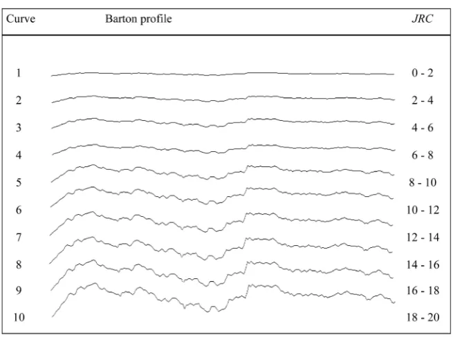
As was said in Introduction, subjective visual comparison a fracture rock surface to be analyzed with the standard Barton profiles (see Figure 1) is preferred way for determining JRC values. Objective methods for JRC are searched, unfortu-nately, many of them are incorrect.

Many researchers believe that the surface roughness of rock joints needs to be characterized using scale invariant parameters such as fractal parameters. Several researchers have suggested using the fractal dimension to quantify rock joint roughness (see [7]-[13] for example).

In [14], there is “derived” a “direct relationship” between the JRC index and fractal dimension D

(

)

50 1

JRC≈ ⋅ D− (2)

[image:2.595.210.538.464.708.2]

However, it is a nonsense as the following example illustrates.

DOI: 10.4236/apm.2017.711037 617 Advances in Pure Mathematics Example: A fractal dimension is namely affine invariant, i.e. each bijective af-fine transformation of the profile has the same dimension as an original. The profile p x

( )

in Figure 2 was generated as a fractional Brownian motion and

for every x is P x

( )

= ⋅4 p x

( )

. To easily determine the dimension of the

result-ing fractal, a random number must be generated by the Gaussian distribution

( )

0;1

N and the i-th iteration step variations σ_i have to be adjusted in

accor-dance with

2

2 0

2

2

i Hi

σ

σ = ₍₃₎

where H∈ 0;1 is so called Hurst exponent.

Due to affine invariance, both profiles have the same dimension (D=1.5) and should have the same roughness therefore. This is evidently not true. More-over, JRC of both profiles is JRC≈25 according to (1). This is also not true.

In [14] [15], another „direct relationship” between dimension and JRC was published:

2

1 1

0.87804 37.7844 16.9304

0.015 0.015

D D

JRC= − + ⋅_ − _− ⋅_ − _

    (4)

[image:3.595.205.539.444.727.2]

This relationship is often cited (see [16] [17] [18] [19] for example) but it is quite false. Equation (4) gives a totally nonsensical results for Barton profiles as will be shown in 2.5 (see the last column of Table 3).

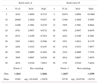
Table 1. Hausdorff dimension and grid measure of the original Koch curve A and its af-fine representation B estimated by box-counting method and power-function method. Used affinity is

[ ] [

x y; → x; 2y

]

.

Koch curve A Koch curve B

ε N (ε) ln(ε) ln(p) ε N (ε) ln(ε) ln(p)

5 4322 1.6094 8.3715 5 32474 1.6094 10.3882

10 20449 2.3026 9.9257 10 13364 2.3026 9.5003

15 12296 2.7081 9.4170 15 7978 2.7081 8.9844

20 8701 2.9957 9.0712 20 5470 2.9957 8.6070

25 6512 3.2189 8.7814 25 4222 3.2189 8.3481

30 5201 3.4012 8.5566 30 3351 3.4012 8.1170

35 4250 3.5553 8.3547 35 2718 3.5553 7.9077

40 3585 3.6889 8.1845 40 2316 3.6889 7.7476

45 3049 3.8067 8.0226 45 2014 3.8067 7.6079

50 2674 3.9120 7.8913 50 1743 3.9120 7.4634

Power. f. Box-counting Power. f. Box-counting

Dim. 1.2621 1.2662 1.2627 1.2599

[image:4.595.210.537.77.137.2]

DOI: 10.4236/apm.2017.711037 618 Advances in Pure Mathematics Figure 2. The profile p x

( )

was generated as a fractional Brownian motion. Due to af-fine invariance, the profiles p x

( )

; P x

( )

have the same dimension but evidently dif-ferent roughness.

We can often read that for computing of fractal dimension, it is necessary to decide whether the object is self-similar or self-affine (see [20] [21] [22] [23]). It is said that “the computation of fractal dimensions of self-affine fractals requires modified computational methods” [14] [20] and their dimensions D have to be computed by others methods than the dimension of self-similar curves. Alleged reason is “different scaling” in the x-and y-directions which changes its dimen-sionality (see [14] for example). However, it is a deep mistake. One example for all: The curve B in Figure 3 contains two its copies with the same scaling (red and pink). These copies required “non-modified” method. However, the same curve contains two copies with different scaling (green and blue). These copies required “modified” method. Can we use the modified or the non-modified me-thod for its dimensionality estimation?

3. Hausdorff Measure and Hausdorff Dimension

Hausdorff defined the first dimension that allows non-integer values. Hausdorff s-dimensional outer measure of a set A is defined as

( )

( )

(

)

; ; ;

1 lim inf

n i

s s

n i n i

n A A

i I

H A diam A diam A

n

∗

→∞ ⊆ _∈

 

=  ≤ 



∑



 (5)

where I is an at most countable index set. Restriction of ( )s

H to the sets

mea-surable with ( )s

H

∗ _{(H-measurable sets) is called Hausdorff s-dimensional} measure of the set A. The number

( )

{

{ }

( )

( )

}

{

{ }

( )

( )

}

0 0

sup d inf 0

H

d

D A = d∈+ ∞ H A = ∞ = d∈+ ∞ H A = (6)

is called Hausdorff dimension of the set A.

Mandelbrot [24] defined fractal as a set which Hausdorff dimension is sharply greater than the topologic dimension. Ever after several dimension which allows non-integer values was defined (see [25] for example). Each of them is called the fractal dimension.

For estimation of the Hausdorff dimension of sets which are constructed on digital devices, so called grid measure and grid dimension are used. The grid s-dimensional outer measure is defined as

( )

( )

(

)

;

; ;

1 lim inf

n i

s s

n i n i

n A A

i I

G A diam A diam A

n

∗

→∞ ⊆ _∈

 

= _ = _



∑



DOI: 10.4236/apm.2017.711037 619 Advances in Pure Mathematics

[image:5.595.242.505.76.181.2]

(a) (b)

Figure 3. “Different scaling” in x- and y-directions can change the self-similar set (a) to self-affine set (b). However, “different scaling” in x- and y-directions can change the self-affine (b) to self-similar set (a).

Its restriction ( )s

G to the sets measurable with ∗G( )s (G-measurable set) is called the grid measure. The grid dimension (G-dimension) of the set A is de-fined as

( )

{

{ }

( )

( )

}

{

{ }

( )

( )

}

0 0

sup d inf d 0

G

D A = d∈+ ∞ G A = ∞ = d∈+ ∞ G A = (8)

The G-dimension is suitable for digital data and since the limit condition n→ ∞ in Formula (7) cannot be realized, the limit is omitted and the Formula (7)is replaced with the approximate equality

( )

( )

(

)

; ; ;

1 inf

n i

s s

n i n i

A A i I

G A diam A diam A

n

∗

⊆ _∈

 

≈ _ = _



∑



 (9)

4. Box Counting and Power-Function Method

For the infimum to be computed in (9), only those sets An i; are taken to the union An i; for which An i; A≠ ∅. Due to the fact that only bounded sets (or more precisely their approximations containing finite elements) can be represented in the computer, the system

{ }

An i; is always finite. Let us denote its

cardinality by N n

( )

. The measured approximations are always G-measurable.

In software implementations of the measurement, used metric is a square metric, where the diameter of a square is equal to its side. According to Formula (9) we obtain for measure in Hausdorff dimension

( )

( )

( )

(

)

( )

( )

;

1 1

1

N n N n

D

D D

n i D

i i

G A diam A N n n

n

−

= =

≈

∑

=

∑

= ⋅ ₍₁₀₎

Therefore,

( )

( )D D

N n ≈G ⋅n (11)

Applying the logarithm on both sides of the approximate equality (11) we ob-tain

( )

( )

lnN n ≈ ⋅D lnn+lnGD (12)

Measuring with a specified n, a N n

( )

is obtained for a covering of the

measured set. The values D and ( )D

DOI: 10.4236/apm.2017.711037 620 Advances in Pure Mathematics

( )

ln ln N n D n

≈ ₍₁₃₎

and even define the dimension as the limit of that fraction, i.e.

( )

ln lim ln B n N n D n →∞

= ₍₁₄₎

This dimension and the method for its measurement are known as the box counting.

Note that n is the reciprocal value of the diameter of covering sets, which is often marked as ε. Therefore, if we denote the cardinality N n

( )

of the

cover-ing of the set to be measured as N

( )

ε

, we obtain

( )

( )D

( )

D

N

ε

≈G A ⋅

ε

− (15)

from (11)

( )

( )

( )

lnN

ε

≈ − ⋅D ln

ε

+lnGD A (16)

from (12) or

( )

1 0 ln lim ln B N D ε ε ε− → +

= ₍₁₇₎

from (14) respectively.

To calculate this dimension for the fractal F, it is necessary to insert this frac-tal into an evenly spaced grid and count how many squares (2D case) or boxes (3D case) are required to cover the set. The box-counting dimension is calcu-lated by seeing how this number changes as we make the grid finer by applying a box-counting algorithm.

It is possible to shown that the theoretically defined box counting dimension (14) is equal to the Hausdorff dimension—see Formula (8). A problem is that the dimension (14) has to be estimated with the least-square method form the linear function (12). If we denote the power function (11) as

( )

D

f x = ⋅G x , sum

of its residues is

( )

( )

2

Σ

n

R = _N n −f n _ , while sum of residues for the linear

function (12) is _*

( )

( )

2

Σ ln ln

n

R = _ N n − f n _ . Of course R*nRn . Thus the

box-counting method systematically overestimates residues of low values and unde-restimates residues of its high values. Moreover, negative values of the difference

( )

( )

lnN n −lnf n have lower weights than positive values. This somehow

low-ers the tangent of the straight line as thus the value of the estimated dimension. This problem can be overcome by searching for the power function (11) in-stead of the linear function (12). The least square method requires in this case minimization of the function

(

)

(

)

2

, D

n

f N D =

∑

N− ⋅G n (18)

This leads to the equation

(

)

2

(

2

)

ln ln 0

D D D D

n n n n

Nn n n − Nn n n =

∑

∑

∑

∑

(19)

DOI: 10.4236/apm.2017.711037 621 Advances in Pure Mathematics

5. Self-Similarity and Self-Affinity

Many technical papers describe the fractals. We can read that the fractals can be either self-similar or self-affine and the original box counting method is a self-similar method and it provides accurate results only for self-similar profiles. Natural rock joint profiles are self-affine, therefore, the box-counting method is not useable for their fractal dimension—see [27] for example. However, these af-firmations are very inaccurately. It is said that self-affine curves, in contrast to self-similar ones, are not identically scaled in x- and y-directions (see [14] [20] [21] [22] for example). This “definition” is unprofessional and very narrow (re-stricted). Many others fractals are self-affine.

A self-affine fractal is any fractal F, for which there exist affine mappings ; 1; 2; ;

i i n

ϕ =  so it holds

( )

1 1

n n

i i

i i

F ϕ F F

= =

=



=



₍₂₀₎

If all affinities ϕi are the similarities then the self-affine fractal is

concur-rently self-similar. It means that the self-similarity is a special case of the self-affinity, i.e. each self-similar set is self-affine concurrently.

In Euclidean space, each affinity is given by

i i

X′ =F ⋅X+v (21)

where Fi is any square matrix and v is any vector. If

T 2

i⋅ i =

λ

⋅

F F I (22)

(where I is the identity matrix) then the affinity is called the similarity, number λ is its coefficient. Except self-similar and self-affine fractals, there exist sets which are neither self-similar nor self-affine (Mandelbrot set for exam-ple).

According of the definition of the Hausdorff dimension is

( )

( )

(

)

; ; 1 0 inf nk k s

n i n i

A A

D

k I

H A diam A diam A

n

⊆ _∈

 

< = _ ≤ _< ∞



∑



 (23)

If a set A is self-similar and λ λ1; 2;;λp are coefficients of the similarities

i

ϕ from (20), and for each i≠ j is H( )D

(

ϕ

i

( )

A 

ϕ

j

( )

A

)

=0 then

( )

( )

(

)

(

)

( )_{( )} ; ; 1 1 inf inf diam nk k nk D k D

n i n i

A A k I p D D i A A H A D i

H A diam A diam A

n A λ ⊆ _∈ ⊆ ₌   =  ≤    =

∑

∑

   (24)

It means that

( )

( )

( )

( )

1 p D i i D D

H A H A λ

=

= ⋅

∑

₍₂₅₎

1 2 1

D D D

p

λ

+

λ

+ +

λ

= (26)

DOI: 10.4236/apm.2017.711037 622 Advances in Pure Mathematics 1 2 ln 1 1 ln

D D D D

p

p

p D

λ

λ

λ

λ

λ

+ + +_ = ⋅ = ⇒ = ₍₂₇₎

Example: the Koch curve is self-similar with four copies of itself, each scaled by the factor one third, its dimension is ln 4

ln 3

D= . The Sierpinski triangle or Sierpinski square are also self-similar with three copies scaled by one half or eight copies scaled by one third respectively, their dimensions are ln 3

ln 2

D= or

ln 8 ln 3

D= respectively.

For H-measure of any fractal, the H-measure of its covering C _nk

kA

=



is determinative. This covering consists of cubes in case of square metric. The measure of self-affine fractals (19) is equal to the sum of measures its affine copies ϕi. Each affinity ϕi transforms a cubical covering C to the set of

parallelepipeds

ϕ

_i

( )

C . We have to find how the volume of cube will change by its transform to the parallelepiped.

Each cube is given by orthonormal vectors a=

(

a a a1; 2; 3

)

; b=

(

b b b1; ;2 3

)

;

(

c c c1; ;2 3

)

=

c which are transform to linearly independent vectors a′=

(

a a a1′ ′ ′; 2; 3

)

;

(

b b b1; ;2 3

)

′= ′ ′ ′

b ; c′=

(

c c c₁′ ′ ′; ;_{2 3}

)

by bijective affinity ϕ_i, i.e.

T T T T T T

; ;

i i i

′ = ⋅ ′ = ⋅ ′ = ⋅

a F a b F b c F c (28)

or

T T T T

; ;

i i i

′= ⋅ ′= ⋅ ′= ⋅

a a F b b F c F c (29)

where Fi is the matrix of the affinty ϕi. This implies

(

1 2 3

) (

1 2 3

)

1112 2122 3132

(

(

1

) (

2

) (

3

)

)

13 23 33

; ; ; ; ; ; ; ; ;

z z z

a a a a a a z z z

z z z

 

 

′ ′ ′ = ⋅_{ }=

 

 

a f a f a f (30)

By analogy

(

b b b1′ ′ ′ =; ;2 3

) (

(

b f; 1

) (

; b f; 2

) (

; b f; 3

)

)

(31)

(

c c c1′ ′ ′ =; ;2 3

) (

(

c f; 1

) (

; c f; 2

) (

; c f; 3

)

)

(32)

Volume of the parallelepiped which is given by vectors a b c′ ′ ′; ; is equal to the scalar triple product. Therefore, we obtain

(

) (

) (

)

(

) (

) (

)

(

) (

) (

)

1 2 3 1

1 2 3 1

1 2 3 1

1 2 3 11 21 31 1 2 3 12 22 32 1 2 3 13 23

2 3 2 3 2 3 33 ; ; ; ; ; ; ; ; ;

a a a

b b b

c c c

a a a f f f

b b b f f f

c c c f f f

′ ′ ′

′ ′ ′ =

′ ′ ′

= ⋅

a f a f a f

b f b f b f

c f c f c f

(33)

from (30), (31), (32). Therefore

(

)

T

(

)

(

)

; ; det i ; ; det i ; ;

DOI: 10.4236/apm.2017.711037 623 Advances in Pure Mathematics It is possible to obtain

(

;

)

det i

( )

;

S a b′ ′ = F⋅S a b

for the area of the parallelogram in two-dimensional space. The diameter of cube (or square) which have the same volume (or area) in square metric is

(

)

3 3

diamAnk′ = detFi ⋅V a b c; ; = detFi ⋅diamAnk (35)

or

( )

diamAnk′ = detFi ⋅S a b; = detFi ⋅diamAnk (36)

respectively.

For the H-measure of a self-affine fractal A which contains p affine copies of itself, we obtain

( )

( )

(

)

(

)

(

)

(

)

(

)

( )_{( )}

(

)

( )

( )

; 1 1 1 1

inf diam diam

1

inf det diam diam

1

inf det diam diam

inf diam det

d nk k nk k nk k nk k D D

n i nk

A A

k I

D

i nk nk

A A

k I

p D _D

i nk nk

A A

i k I

p D D D D nk i A A

k I i

H A

p

i

H A A A

n A A n A A n A H A ⊆ _∈ ⊆ _∈ ⊆ _{= ∈} ⊆ _{∈ =} =   =  ≤      = _ ⋅ ≤ _       = _{  } ≤ _     = =

∑

∑

∑

∑

∑

∑

∑

F F F     

(

et

)

D i F i.e. ( )

( )

( )

( )

(

)

1 det

D D p D

i i

H A H A

=

=

∑

F (37)

Therefore

(

)

1 det 1 p D i i= =

∑

F (38)

and

(

3

)

1 det 1 p D i i= =

∑

F (39)

in three-dimensional space by analogy.

DOI: 10.4236/apm.2017.711037 624 Advances in Pure Mathematics Bijective affine transform (scaling in one direction for example) changes the measure of the transformed set but it does not change its dimensionality. For these measurement, the same methods may be used (without any modification). We estimated the dimensionality and measure of the Koch curve (see Figure 3), i.e. namely the self-similar original A and further its self-affine scaling

[ ] [

]

: ; ; 2

B x y → x y . The box counting method and power function method with

the same parameters are used in both cases. Both curves have been generated as image with resolution 4096 4096× pixels. Results of these measurement are summarised in Table 1 and graphically represented in Figure 4 (box counting) and Figure 5 (power function). For both curves (self-similar and self-affine), approximately the same dimension has been measured (D≈1.26) using two methods (box counting and power function) with the same parameters (ε=5,10,, 50) and withouth any modification. Theoretical dimension is

ln 4

2.261859 ln 3

D= =  in both cases.

Straightlines (in case of the box counting) or power curves (in case of the power function) differs in shifting (extension) in vertical direction only. By this shifting (extension), set measure in corresponding fractal dimension is determined. Remind that the measure is the length in case of D=1 which is

measured in linear micrometers (μm1_{) for example. In case of D=2, the} measure is caled the area which is measured in square micrometers (μm2_{) for} example. In case of Koch curve which dimension is ln 4

ln 3

D= , we must measure

in micrometers powered by ln 4

ln 3

[image:10.595.211.539.470.688.2]

D= . If we presume that the pixel is a square with a side 1 μm then the measure of the curve A is

[image:11.595.210.536.72.284.2]

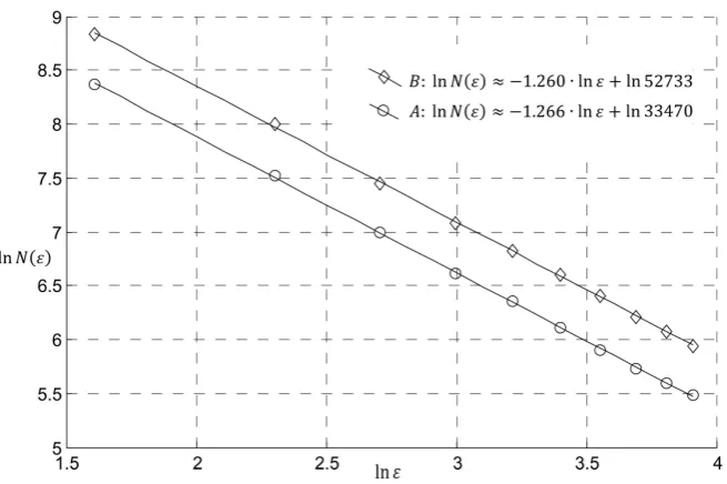
DOI: 10.4236/apm.2017.711037 625 Advances in Pure Mathematics Figure 5. Hausdorff dimension and grid measure of the Koch curve A and its affine re-presentation B. Power-function method, used affinity is

[ ] [

x y; → x; 2y

]

.

( )

( )

(

)

exp 10.4184 33470 m

D D

G A ≈ ≈ µ (40)

according to box counting method and

( )D

( )

_{33365 m}D

G A ≈ µ (41)

according to power function method. For the affine representation B of the curve A, these values are

( )D

( )

_{exp 10.8730}

(

)

_{52733 m}D

G B ≈ ≈ µ (42)

according to box counting method and ( )

( )

52739 m

D D

G B ≈ µ (43)

according to power function method.

For testing of the power function method, following fractals has been chosen: Koch curve, Sierpinski triangle and Sierpinski square (see previous example). The subsequent set (triangle) is constructed as the union of three affine copies of itself, matrices of the affinities—see Equation (21)—are

1 2 3

0.36 0.48 0.36 0.48 0.28 0

; ;

0.48 0.36 0.48 0.36 0 0.28

− −

     

=_{ } =_{ } =_{ }

− − −

     

F F F (44)

(vectors vi are irrelevant for its dimension) then it implies from (38)

(

det 1

) (

det 2

)

(

det 3

)

1

D

D D

+ + =

F F F (45)

in our case

DOI: 10.4236/apm.2017.711037 626 Advances in Pure Mathematics This triangle is self-affine, however it also holds

T T 2 T 2

1 1 = 2 2 =0.6 ⋅ ; 3 3 =0.28 ⋅

F F F F I F F I (47)

It means that this fractal is not only self-affine but also self-similar. It consists of two contractions with λ λ1= 2=0.36 and one contraction with λ =3 0.28.

Therefore, we can also use Equation (26)

0.6D+0.6D+0.28D=1 (48) It is the same equation as (46) and gives the same result. This fractal is illu-strated in Figure 6 on the left and it is called “subsequent triangle” in Table 2.

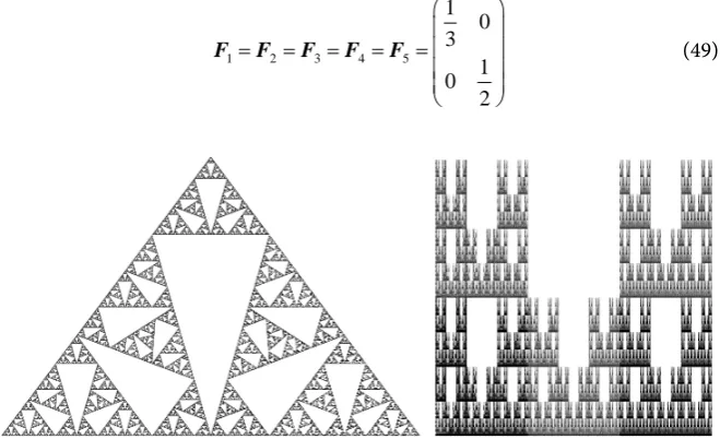
As the next fractal, a self-affine set is constructed (see Figure 6 on the right, it is named as “self-affine square” in Table 2). It contains five affine copies of itself, matrices of the affinities are

1 2 3 4 5

1 0 3

1 0

2

 

 

 

= = = = =

 

 

 

[image:12.595.209.539.261.462.2]

F F F F F (49)

Figure 6. The self-affine triangle and self-affine square.

Table 2. The theoretical dimension of some self-similar and self-affine fractals and the dimension estimated by the power function method.

self- theoretical Dimension _estimated error (%)

Koch curve -similary ln 4 1.2 5

ln 3≈ 618 1.26377 0.152

Sierpinski triangle -similary ln 3 1.5 6

ln 2≈ 849 1.58466 0.019

Sierpinski square -similary ln 8 1.8 9

ln 3≈ 927 1.88729 0.291

Subsequent triangle -similary 1.62234 1.62342 0.067

Self-affine square -affine 1.79649 1.79134 0.287

Barnsley fern -affine 1.76462 1.76249 0.121

Tree -affine 1.81616 1.80511 0.612

[image:12.595.212.540.527.728.2]

DOI: 10.4236/apm.2017.711037 627 Advances in Pure Mathematics its dimension is

(

)

5

1

1 ln 5

det 1 5 1 2 1.796488

6 ln 6

D D

i i

D

=

 

= ⇒ ⋅_ _ = ⇒ = ⋅ ≈

 

∑

M  (50)

Sixth set in Table 2 is the Barnsley fern (see Figure 7 on the left), it has the af-finity matrices

1 2 3 4

0.01 0 0.2 0.2 0.1 0.3 0.83 0.05

; ; ;

0 0.2 0.3 0.2 0.3 0.2 0.05 0.83

− −

       

=_{ } =_{ } =_{ } =_{ }

−

       

F F F F (51)

According to (37) its dimension is D=1.764625

Seveth tested fractal is a tree (see Figure 7 in the middle) with matrices

1 2

3 4

0.195 0.488 0.462 0.414

; ;

0.344 0.443 0.252 0.361

0.058 0.070 0.637 0 ;

0.453 0.111 0 0.501

−

   

=_{ } =_{ }

−

   

− − −

   

=_{ } =_{ }

−

   

F F

F F

(52)

and dimension D=1.816162

The last fractal-“sea horse” has matrices

1 2

0.8 0.3 0.3 0.3

;

0.3 0.8 0.4 0.3

−

   

=_{ } =_{ }

− − −

   

F F (53)

and dimension D=1.796166 (see Figure 7 on the right).

In Table 2, we can compare these theoretical dimensions of previous eight sets with the dimension which was estimated by the power function method. Data was generated by the IFS method (original resolution 4096 4096× pixels). It is clear that the results of this method are sufficiently precise for both types of fractals.

[image:13.595.212.537.581.701.2]

7. Estimation of Hausdorff Dimension of Barton Profiles

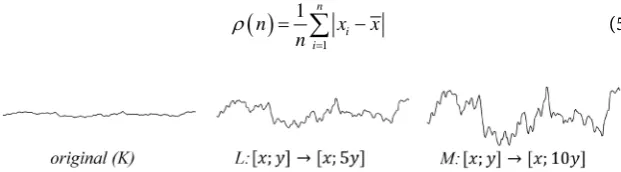
Some authors alerts, that any fractal dimension itself cannot be used for rough-ness modelling (see [7] [28] [29] [30] for example). It is also clear from the ex-ample in Section 2 and from Figure 2. We illustrate this fact also in the case of the Barton Profile.

DOI: 10.4236/apm.2017.711037 628 Advances in Pure Mathematics In Figure 8, we can see the original of fourth Barton profile (K) and its scal-ings L:

[ ] [

x y; → x;5y

]

; M:

[ ] [

x y; → x;10y

]

. These three profiles have been

measured by the power function method with the same parameters.

These measurement are graphically represented in Figure 9. For all three profiles, approximately the same dimension has been measured.

8.

JRC

Estimators

As is clear from previous text, JRC depends not only on the fractal dimension, but also on its statistical variability. Remember that the important variability characteristics are:

The square root of average of the squared differences from the mean, i.e.

( )

(

)

2

1

1 n i i

n x x

n σ

=

=

∑

− (54)

where n is the number of elements of the set, xi are its elements and x is

arithmetic mean (standard deviation) and the arithmetic mean of absolute val-ues of differences between elements of statistical sets and their arithmetic mean, i.e.

( )

1

1 n i i

x x

n n

ρ

=

[image:14.595.217.528.337.423.2]

=

∑

− ₍₅₅₎

Figure 8. The fourth Barton profile and its affine copies.

[image:14.595.214.531.434.670.2]

DOI: 10.4236/apm.2017.711037 629 Advances in Pure Mathematics (average deviation).

The Hurst exponent is directly related to the fractal dimension, which meas-ures the smoothness of a surface, or, in our case, the smoothness of a rock pro-files. The relationship between the fractal dimension D and the Hurst exponent H, is given by

1

H= + −n D (56)

where n is the topological dimension of the measured set (see (59) for example). The Equation (56)—see [31] or [32] for proof—enables to compare the rough-ness in different topological dimensions and also to compare the standard Bar-ton 2D profile with the real 3D profiles to be measured. Therefore, a roughness estimator can be designed to be able to determine the JRC in different topologi-cal dimensions, i.e. the JRC of fractal curves and the JRC of fractal surfaces as well. Therefore, it works with the Hurst exponent for which values is H∈ 0;1 in both cases instead the fractal dimension for which is D∈ 1; 2 in case of the fractal curves and D∈ 2;3 in case of the fractal surfaces.

The JRC is given not only by the Hurst exponent but also by heights of curve or surface irregularities. These irregularities can be quantified using the standard deviation (54) or average deviation (55).

Increasing irregularities heights denotes increasing of the JRC and conversely. Therefore, the standard deviation (53) or average deviation (55) must be placed to numerator of expression to be found. Thus, corresponding formulas are:

E H

σ

σ

= ₍₅₇₎

(standard deviation estimator)

E H

ρ

ρ

= ₍₅₈₎

(average deviation estimator), σ and ρ are given by (54), (55).

For JRC estimation of any profile or surface, so called characteristic functions

( )

JRC_σ E_σ ; and JRC_ρ

( )

E_ρ have been constructed. Each of them has been

de-signed to pass through the origin of the coordinate system (if surface variability is equal to zero then surface is completely smooth horizontal plane, Hurst expo-nent is equal to one and JRC=0). Each of them must be non-negative and in-creasing (as the JRC). Each of them must describe a dependence of the JRC on

E_σ or Eρ respectively and has been found using of the least squares method.

9. Estimation of the Characteristic Functions

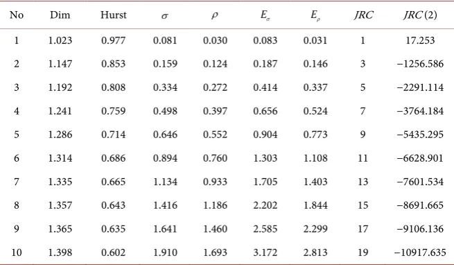
In this section, Hausdorff dimension of all standard Barton profiles has been es-timated using power function method and values of E_σ ; E_ρ for the standard Barton profiles have been measured. Results of these measurements are summa-rized in Table 3.

For JRC estimation of any profile or surface, so called characteristic functions

( )

[image:16.595.210.538.126.317.2]

DOI: 10.4236/apm.2017.711037 630 Advances in Pure Mathematics Table 3. Hausdorff dimensions, Hurst exponents, standard deviations, average devia-tions, standard deviation estimators and average deviation estimators of the standard Barton profiles. In the last column, “JRC” assigned to corresponding dimension by present used and often cited expression (4).

No Dim Hurst σ ρ Eσ Eρ JRC JRC (2)

1 1.023 0.977 0.081 0.030 0.083 0.031 1 17.253

2 1.147 0.853 0.159 0.124 0.187 0.146 3 −1256.586

3 1.192 0.808 0.334 0.272 0.414 0.337 5 −2291.114

4 1.241 0.759 0.498 0.397 0.656 0.524 7 −3764.184

5 1.286 0.714 0.646 0.552 0.904 0.773 9 −5435.295

6 1.314 0.686 0.894 0.760 1.303 1.108 11 −6628.901

7 1.335 0.665 1.134 0.933 1.705 1.403 13 −7601.534

8 1.357 0.643 1.416 1.186 2.202 1.844 15 −8691.665

9 1.365 0.635 1.641 1.460 2.585 2.299 17 −9106.136

10 1.398 0.602 1.910 1.693 3.172 2.813 19 −10917.635

signed to pass through the origin of the coordinate system (if surface variability is equal to zero then surface is completely smooth horizontal plane, Hurst expo-nent is equal to one and JRC=0). Each of them must be non-negative and in-creasing (as the JRC). Each of them must describe a dependence of the JRC on

E_σ or Eρ respectively and has been found using of the least squares method.

Equations of these functions are

( )

0.651

9.186

JRC_σ E_σ = ⋅E_σ (59)

(see Figure 10)

( )

0.612

10.095

JRC_ρ E_ρ = ⋅E_ρ (60)

(see Figure 11).

10. Estimation of the

JRC

Index of Real Samples

All geological data used in this paper has been acquired by prof. Tomáš Ficker from the Faculty of Civil Engineering of our university. All the samples are spe-cimens of limestone (locality Brno-Hády, Czech Republic). All processing and visualization of these data have been made by original author’s software. For more information of these reconstructions and visualizations see [33] [34] [35] [36].

[image:17.595.215.532.71.295.2]

DOI: 10.4236/apm.2017.711037 631 Advances in Pure Mathematics Figure 10. The JRC as function of standard deviation estimator E_σ—see (59).

Figure 11. The JRC as function of average deviation estimator E_ρ—see (60).

However, the JRC may have different values along different orientations on a rock surface. In this case, we can choose the direction of the JRC estimation. The profile curve is generated for selected direction and its Hausdorff dimension is measured by power function method according to (11). There is D∈

( )

1; 2 ,

2

n= in expression (56) and also H∈

( )

0;1 in expressions (57), (58) which serves for JRC estimation. This JRC we call the directional JRC.

The global JRC has been estimated for the samples A B C D; ; ; from Figure

[image:17.595.213.535.332.548.2]

DOI: 10.4236/apm.2017.711037 632 Advances in Pure Mathematics

(A) (B)

[image:18.595.213.536.78.337.2]

(C) (D)

[image:18.595.253.496.383.499.2]

Figure 12. The limestone samples under tests. 3D reconstruction from the series of par-tially focused images (see [33] [34] [35] [36] for more information).

Figure 13. Directions that were used for estimation of the directional JRCs of the samples ; ; ;

A B C D. The profiles marked as blue on the left are illustrated on the right.

Results of these measurements are summarized in Table 4 and Table 5 and graphically represented in Figures 14-19. In Figure 14 we can see dimension estimation of the profile with direction 0˚ on the sample A, the profile with di-rection 90˚ on the sample B, the profile with didi-rection 100˚ on the sample C and the profile with direction 200˚ on the sample D using box counting method. In Figure 15, there are illustrated estimation of the same profiles using power func-tion method.

[image:19.595.212.539.129.717.2]

DOI: 10.4236/apm.2017.711037 633 Advances in Pure Mathematics Table 4. Hausdorff dimensions estimated by power function method, Hurst exponents, standard deviations, average deviations and directional JRCs of the samples A B, . Aver-aged values on these quantities are in the second last row, corresponding values of the global JRCs are in the last row.

Angle Sample A Sample B

Dim Hurst σ ρ JRCσ JRCρ Dim Hurst σ ρ JRCσ JRCρ

[image:20.595.212.537.128.724.2]

DOI: 10.4236/apm.2017.711037 634 Advances in Pure Mathematics Table 5. Hausdorff dimensions estimated by power function method, Hurst exponents, standard deviations, average deviations and directional JRCs of samples C D, . Averaged values on these quantities are in the second last row, corresponding values of 3D surface are in the last row.

Angle Sample C Sample D

Dim Hurst σ ρ JRCσ JRCρ Dim Hurst σ ρ JRCσ JRCρ

0˚ 1.318 0.682 3.994 4.156 13.149 12.306 1.087 0.913 2.765 3.232 8.579 8.852 10˚ 1.459 0.541 3.319 3.689 13.564 13.185 1.109 0.891 3.404 3.933 9.970 10.119 20˚ 1.494 0.506 2.909 3.495 12.992 13.275 1.161 0.839 3.511 4.508 10.578 11.403 30˚ 1.455 0.545 3.500 3.411 13.968 12.514 1.157 0.843 3.517 4.607 10.555 11.518 40˚ 1.401 0.599 3.888 4.073 14.063 13.158 1.156 0.844 4.151 4.693 11.743 11.640 50˚ 1.372 0.628 4.749 4.507 15.526 13.598 1.150 0.850 4.427 4.776 12.192 11.718 60˚ 1.399 0.601 4.283 4.656 14.945 14.246 1.117 0.883 4.449 4.821 11.932 11.514 70˚ 1.346 0.654 4.284 4.504 14.137 13.253 1.116 0.884 4.057 4.713 11.232 11.349 80˚ 1.293 0.707 4.260 4.166 13.402 12.064 1.105 0.895 3.730 4.286 10.549 10.631 90˚ 1.415 0.585 3.120 3.356 12.385 11.872 1.132 0.868 2.953 3.397 9.248 9.406 100˚ 1.481 0.519 2.142 2.488 10.491 10.645 1.094 0.906 4.227 4.147 11.351 10.346 110˚ 1.385 0.615 1.939 2.104 8.809 8.670 1.086 0.914 5.082 4.872 12.721 11.350 120˚ 1.396 0.604 1.865 1.846 8.689 8.099 1.103 0.897 5.948 6.555 14.253 13.741 130˚ 1.419 0.581 1.783 1.809 8.656 8.190 1.047 0.953 7.430 10.987 15.831 18.124 140˚ 1.474 0.526 1.609 1.819 8.636 8.729 1.142 0.858 8.048 11.253 17.850 19.603 150˚ 1.398 0.602 1.705 1.797 8.220 7.986 1.059 0.941 9.160 12.247 18.281 19.509 160˚ 1.338 0.662 2.288 2.540 9.345 9.295 1.062 0.938 8.338 10.554 17.234 17.857 170˚ 1.357 0.643 2.630 2.903 10.420 10.256 1.061 0.939 6.999 8.614 15.376 15.776 180˚ 1.270 0.730 3.976 4.447 12.550 12.307 1.050 0.950 5.728 7.242 13.408 14.104 190˚ 1.279 0.721 4.487 4.769 13.679 12.933 1.082 0.918 6.110 6.520 14.293 13.510 200˚ 1.256 0.744 3.871 3.862 12.179 11.164 1.076 0.924 6.594 7.103 14.948 14.170 210˚ 1.341 0.659 2.901 2.715 10.938 9.709 1.104 0.896 7.429 9.604 16.480 17.344 220˚ 1.389 0.611 2.006 1.724 9.038 7.712 1.044 0.956 9.084 12.200 17.998 19.277 230˚ 1.464 0.536 1.476 1.475 8.069 7.599 1.059 0.941 9.968 12.504 19.312 19.758 240˚ 1.293 0.707 2.257 2.359 8.878 8.539 1.047 0.953 9.273 12.537 18.282 19.641 250˚ 1.359 0.641 2.206 2.253 9.322 8.813 1.061 0.939 6.954 7.819 15.318 14.881 260˚ 1.299 0.701 2.556 3.251 9.680 10.432 1.126 0.874 4.916 4.973 12.810 11.803 270˚ 1.258 0.742 2.704 3.393 9.675 10.343 1.156 0.844 3.479 2.549 10.476 8.038 280˚ 1.269 0.731 3.062 3.612 10.589 10.841 1.168 0.832 2.007 1.992 7.402 6.981 290˚ 1.283 0.717 3.271 4.590 11.189 12.685 1.203 0.797 1.653 1.454 6.711 5.918 300˚ 1.229 0.771 4.576 6.858 13.262 15.480 1.223 0.777 2.021 2.052 7.771 7.407 310˚ 1.273 0.727 5.372 7.117 15.294 16.415 1.219 0.781 2.294 2.474 8.410 8.274 320˚ 1.255 0.745 5.775 7.138 15.770 16.198 1.131 0.869 2.798 3.073 8.924 8.845 330˚ 1.224 0.776 5.668 6.636 15.178 15.120 1.154 0.846 2.435 2.700 8.303 8.315 340˚ 1.298 0.702 4.931 5.576 14.793 14.452 1.111 0.889 2.514 2.735 8.205 8.128 350˚ 1.376 0.624 4.124 4.400 14.221 13.445 1.089 0.911 2.406 2.584 7.849 7.736 Aver. 1.350 0.650 3.319 3.708 11.825 11.542 1.112 0.888 4.996 5.953 12.399 12.461

[image:21.595.210.535.69.292.2]

DOI: 10.4236/apm.2017.711037 635 Advances in Pure Mathematics Figure 14. Graphical representation of profile dimension estimation: sample A, direction 0˚, sample B, direction 90˚, sample C direction 100˚, sample D, direction 200˚ (box counting method).

Figure 15. Graphical representation of profile dimension estimation: sample A, direction 0˚, sample B, direction 90˚, sample C direction 100˚, sample D, direction 200˚ (power function method).

1) Directional JRC_σ is marked as red solid

2) Directional JRCρ is marked as green solid

3) Average of directional JRC_σ is marked as red dashed

4) Average of directional JRCρ is marked as green dashed

5) Global JRC_σ is marked as blue

[image:21.595.212.534.351.571.2]

[image:22.595.213.534.75.355.2]

DOI: 10.4236/apm.2017.711037 636 Advances in Pure Mathematics Figure 16. Directional JRC_σ and JRC_ρ, average of directional JRC_σ and JRC_ρ,

global (3) JRC_σ and JRC_ρ of the sample A.

Figure 17. Directional JRC_σ and JRC_ρ, average of directional JRC_σ and JRC_ρ,

[image:22.595.213.533.408.687.2]

[image:23.595.212.535.74.354.2]

DOI: 10.4236/apm.2017.711037 637 Advances in Pure Mathematics Figure 18. Directional JRCσ and JRCρ, average of directional JRCσ and JRCρ, global (3D) JRC_σ and JRC_ρ of the sample C.

[image:23.595.212.535.407.688.2]

DOI: 10.4236/apm.2017.711037 638 Advances in Pure Mathematics

11. Conclusions

This article showed that the fractal dimension does not dependent on scaling. Therefore, there exists no direct relationship between the fractal dimension and JRC, any fractal dimension itself cannot be used for roughness modelling. JRC depends not only on the fractal dimension, but also on other variables. In this paper, statistical variability of the surface has been used. Increasing irregularities heights denote increasing of the JRC and conversely. Therefore, the standard deviation or average deviation must be placed to numerator of the JRC estima-tor.

The JRC estimator is designed to be able to determine the JRC in different to-pological dimensions, i.e. the JRC of fractal curves and the JRC of fractal surfaces as well. Therefore, Hurst exponent was used instead the fractal dimension. In-creasing dimension denotes inIn-creasing roughness and deIn-creasing Hurst expo-nent. Conversely-decreasing dimension denotes decreasing roughness and in-creasing Hurst exponent. For this reason, Hurst exponent must be placed to de-nominator of the JRC is estimator.

The estimator enables fully automatic estimation of the isotropic (global) joint roughness coefficient (this assumes independence on the direction) and also anisotropic (directional) joint roughness coefficient (which value depends on the direction). In case of the isotropic JRC, the estimator works with whole surface which is topologically two-dimensional, in case of the anisotropic JRC, the esti-mator works in chosen direction, i.e. with topologically one-dimensional profile. The average of the anisotropic JRC estimated for 360˚ with step 10˚ is approx-imately equal to the isotropic (global) JRC.

Acknowledgements

This work was supported by the Project LO1202 by financial means from the Ministry of Education, Youth and Sports under the National Sustainability Pro-gramme I.

The author thanks to prof. Tomáš Ficker from the Faculty of Civil Engineer-ing of Brno University of Technology for the provided data.

References

[1] Barton, N. and Choubey, V. (1977): The Shear Strength of Rock Joints in Theory and Practice. Rock Mechanics, 10, 1-65. https://doi.org/10.1007/BF01261801 [2] Tse, R. and Cruden, D.M. (1979) Estimating Joint Roughness Coefficients.

Interna-tional Journal of Rock Mechanics and Mining Sciences, 16, 303-307. https://doi.org/10.1016/0148-9062(79)90241-9

[3] Maerz, N.H., Franklin, J.A., and Bennett, C.P. (1990) Joint Roughness Measurement Using Shadow Profilometry. International Journal of Rock Mechanics and Mining Sciences, 27, 329-343. https://doi.org/10.1016/0148-9062(90)92708-M

[4] Hong, E.-S., Lee, I.-M. and Lee, J.-S. (2006) Measurement of Rock Joint Roughness by 3D Scanner. Geotechnical Testing Journal, 29, 1-8.

DOI: 10.4236/apm.2017.711037 639 Advances in Pure Mathematics Rough Rock Joints. International Journal for Numerical and Analytical Methods in Geomechanics, 32, 1385-1403. https://doi.org/10.1002/nag.678

[6] Fardin, N., Stephansson, O. and Jing, L. (2001) The Scale Dependence of Rock Joint Surface Roughness. International Journal of Rock Mechanics and Mining Sciences, 38, 659-669. https://doi.org/10.1016/S1365-1609(01)00028-4

[7] Brown, S.R. and Scholz, C.H. (1985) Broad Band Width Study of the Topography of Natural Rock Surfaces. Journal of Geophysics Research, 90, 12575-12582.

https://doi.org/10.1029/JB090iB14p12575

[8] Miller, S.M., McWilliams, P.C. and Kerkering, J.C. (1990) Ambiguities in Estimat-ing Fractal Dimensions of Rock Fracture Surfaces. In: Balkema, A.A., Ed., Proceed-ings of the 31st U.S. Symposium, Colorado School of Mines, Rotterdam, June 18-20 1990, 471-478.

[9] Power, W.L. and Tullis, T.E. (1991) Euclidean and Fractal Models for the Descrip-tion of Rock Surface Roughness. Journal of Geophysical Research, 96, 415-424. https://doi.org/10.1029/90JB02107

[10] Huang, S.L., Oelfke, S.M. and Speck, R.C. (1992) Applicability of Fractal Characte-rization and Modeling to Rock Joint Profiles. International Journal of Rock Me-chanics and Mining Science, 29, 89-98.

https://doi.org/10.1016/0148-9062(92)92120-2

[11] Poon, C.Y., Sayles, R.S. and Jones, T.A. (1992) Surface Measurement and Fractal Characterization of Naturally Fractured Rocks. Journal of Physics D: Applied Phys-ics, 25, 1269-1275.https://doi.org/10.1088/0022-3727/25/8/019

[12] Odling, N.E. (1994) Natural Fracture Profiles, Fractal Dimension and Joint Rough-ness Coefficients. Rock Mechanics, 27, 135-153.

https://doi.org/10.1007/BF01020307

[13] Den Outer, A., Kaashoek, J.F. and Hack, H.R.G.K. (1995) Difficulties with Using Continuous Fractal Theory for Discontinuity Surfaces. International Journal of Rock Mechanics and Mining Science, 32, 3-10.

https://doi.org/10.1016/0148-9062(94)00025-X

[14] Ficker, T. (2016) Fractal Properties of Rock Joint Coefficients. International Journal of Rock Mechanics & Mining Science, 94, 27-31.

https://doi.org/10.1016/j.ijrmms.2017.02.014

[15] Lee, Y.H., Carr, J.R., Barr, D.J. and Haas, C.J. (1990) The Fractal Dimension as a Measure of the Roughness of Rock Discontinuity Profiles. International Journal of Rock Mechanics and Mining Sciences, 27, 453-464.

https://doi.org/10.1016/0148-9062(90)90998-H

[16] Li, Y. and Huang, R. (2015) Relationship between Joint Roughness Coefficient and Fractal Dimension of Rock Fracture Surfaces. International Journal of Rock Me-chanics and Mining Sciences, 75, 15-22.

https://doi.org/10.1016/j.ijrmms.2015.01.007

[17] Sanei, M., Faramarzi, L., Goli, S., et al. (2015) Development of a New Equation for Joint Roughness Coefficient (JRC) with Fractal Dimension: A Case Study of Bakh-tiary Dam Site in Iran. Arabian Journal of Geosciencies, 8, 465-475.

https://doi.org/10.1007/s12517-013-1147-3

[18] Li, Y., Oh, J., Mitra, R., et al. (2017) A Fractal Model for the Shear Behaviour of Large-Scale Opened Rock Joints. Rock Mechanics and Rock Engineering, 50, 67-79. https://doi.org/10.1007/s00603-016-1088-8

DOI: 10.4236/apm.2017.711037 640 Advances in Pure Mathematics https://doi.org/10.1137/S0036144501394387

[20] Feder, J. (1988) Fractals. Plenum Press, New York.

[21] Maliverno, A. (1990) A Simple Method to Estimate Fractal Dimension of a Self-Affine Series. Geophysical Research Letters, 17, 1953-1956.

https://doi.org/10.1029/GL017i011p01953

[22] Bovil, C. (1996) Fractal Geometry in Architecture and Design. Birkhäuser, Boston. https://doi.org/10.1007/978-1-4612-0843-3

[23] Stamps, A.E. (2002) Fractals, Skylines, Nature and Beauty. Landscape and Urban Planning, 60, 163-184.https://doi.org/10.1016/S0169-2046(02)00054-3

[24] Mandelbrot, B.B. (1967) How Long Is the Coast of Britain? Statistical Self-Similarity and Fractional Dimension. Science, 156, 636-638.

https://doi.org/10.1126/science.156.3775.636

[25] Hastings, H. and Sugihara, G. (1993) Fractals—A User’s Guide for the Natural Sciences. Oxford University Press, Oxford.

[26] Martišek, D. and Druckmüllerová, H. (2014) Power-Function Method of Fractal Dimension Estimation. 20th International Conference of Soft Computing Mendel Brno, 26-27 June 2014, 147-152.

[27] Kulatilake, P.H.S.W., et al. (2006) Natural Rock Joint Roughness Quantification through Fractal Techniques. Geotechnical and Geological Engineering, 24, 1181-1202. https://doi.org/10.1007/s10706-005-1219-6

[28] Power, W.L. and Tullis, T.E. (1991) Euclidean and Fractal Models for the Descrip-tion of Rock Surface Roughness. Journal of Geophysical Research, 96, 415-424. https://doi.org/10.1029/90JB02107

[29] Brown, S.R. (1987) A Note on the Description of Surface Roughness Using Fractal Dimension. Geophysical Research Letters, 14, 1095-1098.

https://doi.org/10.1029/GL014i011p01095

[30] Brown, S.R. (1995) Simple Mathematical Model of a Rough Fracture. Journal of Geophysical Research, 100, 5941-5952.https://doi.org/10.1029/94JB03262

[31] Mandelborot, B. (1982) The Fractal Geometry of Nature. W. H. Freeman, San Fran-cisco.

[32] Turcotte, D.L. (1992) Fractals and Chaos in Geology and Geophysics. Cambridge University Press, Cambridge.

[33] Martišek, D. (2002) The 2-D and 3-D Processing of Images Provided by Conven-tional Microscopes. Scanning, 24, 284-296.https://doi.org/10.1029/94JB03262 [34] Martišek, D. and Druckmüllerová, H. (2014a) Multifocal Image Processing.

Ma-thematics for Applications, 3, 77-90.https://doi.org/10.13164/ma.2014.06

[35] Martišek, D., et al. (2015) High-Quality Three-Dimensional Reconstruction and Noise Reduction of Multifocal Images from Oversized Samples. Journal of Elec-tronic Imaging, 24, Article ID: 053029.https://doi.org/10.1117/1.JEI.24.5.053029 [36] Martišek, D. and Druckmüllerová, H. (2017) Registration of Partially Focused