Munich Personal RePEc Archive
Firm Heterogeneity and the Pattern of
RD Collaborations
Billand, Pascal and Bravard, Christophe and Durieu, Jacques
and Sarangi, Sudipta
Virginia Tech
August 2018
Online at
https://mpra.ub.uni-muenchen.de/89247/
Firm Heterogeneity
and the Pattern of R&D Collaborations
1Pascal Billand
a, Christophe Bravard
b, Jacques Durieu
b, Sudipta Sarangi
caUniversit´e de Lyon, Lyon, F-69003, France ; Universit´e Jean Monnet, Saint-Etienne, F-42000, France;
CNRS, GATE Lyon St Etienne, Saint-Etienne, F-42000, France; pascal.billand@univ-st-etienne.fr
b Universit´e Grenoble-Alpes, GAEL, GATE Lyon St Etienne; christophe.bravard@univ-grenoble-alpes.fr,
jacques.durieu@univ-grenoble-alpes.fr
cDIW Berlin and Department of Economics, Virginia Tech Blacksburg VA 24061 - 0316, USA;
ssarangi@vt.edu.
August 2018
Abstract
We consider an oligopoly setting in which firms form pairwise collaborative links in R&D with other firms. Each
collaboration generates a value that depends on the identity of the firms that collaborate. First, we provide properties
satisfied by pairwise equilibrium networks and efficient networks. Second, we use these properties in two types of
situation (1) there are two groups of firms, and the value of a collaboration is higher when firms belong to the same
group; (2) some firms have more innovative capabilities than others. These two situations provide clear insights
about how firms heterogeneity affects both equilibrium and efficient networks. We also show that the most valuable
collaborative links do not always appear in equilibrium, and a public policy that increases the value of the most
valuable links may lead to a loss of social welfare.
JEL classification: C70, L13, L20;
Key Words: Networks, R&D collaborations, link value heterogeneity.
1
1
Introduction
R&D collaboration among firms is now quite widespread, especially in industries characterized by
rapid technological change like pharmaceutical, chemical and IT industries. Interestingly vast
ma-jority of these collaborations are bilateral (see for instance Hagedoorn, 2002), prompting questions
about the structural features of the network of R&D collaborations and their impact on industry
performance (Powell et al. 2005). The architecture of these networks is typically asymmetric.
More-over, it is often possible to find the simultaneous co-existence of firms having intense collaborations
with other firms engaging minimally in collaborative activities (Powell et al. 2005). Another key
feature that comes across from the empirical literature is that the identities of the collaborating
firms is important for understanding the resulting networks (see for instance Vonrotas and Okamura,
2009, Vonortas, 2015).
Keeping these stylized facts in mind, our paper develops a model of R&D collaboration among
horizontally related firms where the outcome of the collaboration depends on the characteristics or
identity of the firm (as shown in Mowery et al. 1998 and Gomes-Casseres, Hagendorn and Jaffe,
2006). The paper incorporates an interesting trade-off: while interfirm collaboration lowers costs
of production, it also serves to increase competition among rival firms. Following Goyal and Joshi
(2003; henceforth GJ), we set up a two oligopoly stage model where firm establish their collaborative
links in stage 1 and compete in stage 2. The pairwise collaborative links for R&D purposes in our
model require a commitment of resources on the part of the collaborating firms, viewed as the costs
of link formation, and lead to lower production costs. The cost-reducing impact of collaborations
is link-specific to capture the identity of the firms in question.2
We begin by examining the classic homogeneous product model of quantity competition and
identify properties of the equilibrium and efficient networks for this case. This helps to establish
results for our main question of interest: what is the architecture of stable and efficient networks?
Given that our model allows for link specific heterogeneity, a systematic technique is needed to
obtain insights about the pattern of collaborations that will occur in equilibrium networks and
welfare-maximizing networks. We do this by introducing two stylized frameworks where we limit
the heterogeneity in the cost-reduction parameter in a systematic way. These frameworks allow to
take into consideration two types of heterogeneity that are often cited as playing an important role
in the choice of collaborative partners and the result of collaborations (see among others Mowery et
al., 1998, Gomes-Casseres, et al., 2006, Vonortas and Okamura, 2009, Vonortas and Zirulia, 2015,
Blum et al., 2017).
(1) In the Insider-Outsider framework (I-O framework), we assume that firms belong to two
distinct groups and the value of a collaboration between two firms is higher if these firms belong to
the same group than if they belong to different groups. This allows us to have two possible levels
of cost-reduction. Such an heterogeneity highlights the role of different kinds of proximities (e.g.,
technical, geographical, ...) between firms in the choice and the value of interfirm collaboration.
(2) In the High and Low innovative firms framework (H-L framework), we assume that firms
either have high or low innovative potential. The value of collaboration between high innovative
potential firms is higher than the corresponding value between two low innovative potential firms.
The cost of production when a firm with innovative potential collaborates with a firm having low
innovative potential lies in between the other two costs. Thus in this framework, we have three
different cost reduction parameters. This framework relies on the well-established facts that firms
differ in their posture toward innovation and that firms with a more dynamic posture toward
innovation are more attractive as collaborative partners.3
Architectures that arise in equilibrium networks in these two frameworks are either of a
group-dominant type or of a hierarchical type.4 We then identify the architectures of efficient networks
3The I-O framework can be seen as an horizontal heterogeneity and the H-L framework as a vertical heterogeneity.
We thank one of the referees for this distinction.
4In a group-dominant type architecture, there are sets of firms such that firms belonging to a set are linked with
in the I-O and H-L frameworks.5 We establish that in both frameworks efficient networks are of a
nested split graph/network type.6 Finally, we go beyond the linear oligopoly model and demonstrate
how our results can be generalized to a larger class of games that includes both the differentiated
Cournot and Bertrand oligopoly models.
Our paper is a contribution to the study of network formation and cooperation in oligopolies.
The model of collaborative networks we present is inspired by recent research on R&D networks
and is most directly related to GJ (2003). The authors assume that collaborative R&D links
are homogeneous, that is they have the same value in terms of their cost-reducing impact. Our
model depart from this assumption, and considers by allowing for the value of the cost-reducing
parameter to vary across links, and provides a systematic way to obtain insights under links cost
heterogeneity. Additionally, since our model incorporates the identity of the collaborating firms, we
find that the pattern of equilibrium networks is asymmetric, which is closer to reality. In the GJ
model, in equilibrium, either all firms are similar (form a complete network or an empty network),
or there are two groups of firms (in the group-dominant network). However, in the latter case, firms
belonging to a group have the same number of links, therefore have the same marginal cost and
competitiveness in the market. The introduction of link-specific heterogeneity in our paper implies
a much greater variability in the degree of competitiveness among firms. In particular, with just
two different sets of link values, hierarchical architectures already emerge in equilibrium.
Finally, our model also allows us to give some interesting insights over public policy. In the paper,
we find that the most valuable links are not always formed in equilibrium networks. This implies
that more profitable innovations do not always occur in equilibrium. However we show that public
intervention aimed at promoting the most valuable links can be counterproductive.
Our paper also relates to Westbrock (2010) who provides architectures of efficient networks for
5Note that while we only consider two types of firms in the I-O and H-L frameworks, our results are qualitatively
preserved when we allow for a greater number of firm types. 6
homogeneous link values. Billand et al. (2015) refine his result and show that efficient networks are
nested split graphs using conditions on individual firm payoffs rather than aggregate payoffs.7 Our
paper finds the conditions on individual payoffs when link values are heterogeneous.
We now briefly point out some other papers to which our work relates as well. Goyal and
Moraga-Gonzales (2001), Goyal, Moraga-Gonzales, and Konovalov (2008) analyze the interaction
between the effort of firms on collaborative links and the effort of firms on other R&D projects,
under link cost heterogeneity. Our paper also complements the work of K¨onig et al. (2012) who
examine stability and efficiency of R&D networks in a model with network dependent spillovers.
The presence of both direct and indirect spillovers in the analysis of K¨onig et al. is an important
feature of their model that distinguishes it from the GJ’s framework. Not surprisingly, in their
paper, because of the benefits from indirect links, every firm in a connected component has the
same profit.
The rest of the paper is organized as follows. In section 2, we present the model setup. In section
3, we provide the results for a market with homogeneous products under quantity competition. In
section 4, we propose a generalized framework which allows us to deal with differentiated oligopolies.
In section 5, we conclude and also discuss the differences between our framework and heterogeneous
link formation costs.
2
Model setup
Network definitions. We consider an industry with a set N ={1, . . . , n} of firms. In the game we model, every firm first announces its intended R&D collaboration links: si,j = 1 means that
firm iintends to form a collaborative link with firm j, andsi,j = 0 otherwise. Firms only play pure
of firm i. The set S =×j∈NSj is the set of strategy profiles of firms. A link ij between two firmsi
and j is formedif and only if si,j =sj,i= 1. A strategy profile s={s1, s2, ..., sn} therefore induces
a network g[s]. For expositional simplicity we will often omit the dependence of the network on the
underlying strategy profile. A network g is a formal description of the pairwise links, representing R&D collaboration, that exist between the firms. If firms i and j are linked in g, we say ij ∈ g, and we say ij 6∈g otherwise. The number of links in g is denoted by|g|.
Let g(i) be the set of firms with whom i has formed a link. The cardinality of g(i), denoted by
|g(i)|, is called the degree of firm i. We denote byN(g) the set of firms that are involved in at least one link in g. We set g−i as the network formed when firm i and its links are deleted, g+ij as the
network obtained when the link ij is added to g, andg−ij as the network obtained when the link
ij is removed fromg.
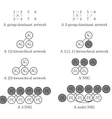
Network architectures. The empty network is the network with no links. The complete network is the network where every firm iis linked with each other firm. In the paper, we also find other equilibrium network architectures, some of them are illustrated in Figure 1. In the figure,
every circle represents a set of firms who have the same neighbors; these firms have formed the same
number of links. If a circle is shaded in white, then firms belonging to the set associated to this
circle are all linked together, while there are no links between these firms when the circle is shaded
in grey. Moreover, a line between two sets of firms, say N1 and N2, indicates that there is a link
between any two firms i∈ N1 and j ∈ N2.
In a group-dominant network, there is a set of firms that are all linked together and there are no
other links. In a 2-group-dominant network, there is a partition ofN(g) in two sets, such that firms that belong to a set are linked together, but there are no other links.
In a 2|2-hierarchical network there is a partition of N(g), {N1,N2,N3,N4}, such that firms that
belong to a set are all linked together, and firms in N1 and N2 are linked together. Moreover,
j ∈ N4, and there are no other links. Firms in N1 and N2 are called influential firms, and firms in
N3 and N4 are called influenced firms. In a 1|2-hierarchical network there is a partition of N(g),
{N1,N2,N3}, such that firms that belong to a set are all linked together, each firmi∈ N1 is linked
with every firm in j ∈ N2 ∪ N3 and there are no other links. Firms that belong to N1 are called
influential firms. A 1|(1,1)-hierarchical networkis similar to a 1|2-hierarchical network except that there are no links between firms in N3.
In the paper, we find that efficient networks are nested split graph (NSG) types. Basically, in
a NSG, the neighborhood of a node is contained in the neighborhoods of the nodes with higher
degrees.8 The nested property implies that there is a partition of firms (D
0, D1, . . . , Dm) such that
firms which belong to Dℓ, ℓ∈ {0, . . . , m−1}, have a lower degree that firms which belong to Dℓ+1.
In a 2-NSG there is a partition of N(g), {N1,N2}, such that firms in each set form a NSG. The
NSG property implies that there is a partition of firms in group k, k = 1,2, (Dk
0, D1k, . . . , Dmk) such
that firms which belong to Dk
ℓ have a lower degree that firms which belong to D k
ℓ+1. A multi-NSG
is a 2-NSG, with firms in N1 and firms in N2 forming a NSG, and each firm i∈ D41 (D42) is linked
with all firms i′ that are linked with a firm j ∈ D1
3 (D32). A group-NSG is similar to a multi-NSG
except that there are no links between firms in N2.
Values of links. To capture heterogeneity inherent in R&D collaboration, we assume that each R&D collaboration is valued differently by the firms. Since R&D collaborations (viewed as
link) reduce costs for the firm, we assume that different R&D collaborations can reduce costs to
different extents. This captures the idea that the innovation targeted by one link is different from
the innovation targeted by another link. Let vi,j >0 be the exogenously given value of the linksij
for the firm i. We assume that a link between two collaborating firms i and j has the same value for the two firms involved, that is vi,j = vj,i, and we set ¯v = max{vi,j}. In the following, we say
that link ij is more valuablethan link i′j′ if v
i,j > vi′,j′.
1 2
3 4
5 6
7 8
1 2
3 4
5 6
7 8
A group-dominant network A 2-group-dominant network
1
N3 N2
N1
N2
N1
N3
A 1|2-hierarchical network A 1|(1,1)-hierarchical network
1
N4 N2
N1
N3 D3 D4
D1 D2 D0
A 2|2-hierarchical network A NSG
D1
3 D41 D23 D42
D1 1 D21
D1 0
D2
1 D22 D20
D1
3 D41 D23 D42
D1 1 D21
D1 0
D2
1 D22 D20
[image:9.612.108.469.189.571.2]A 2-NSG A multi-NSG
We associate with each firm i a number Vi(g) = P
ij∈g(i)vi,j representing its “flow degree”. We
set V(g) =Pij∈g,i>jvi,j the sum of the flow degree of firms, and V(g−i) =V(g)− Vi(g) the sum of
the flow degree of firms in network g−i.
Structure of the game. The game played by the firms consists of two stages.
1. Stage 1: Firms simultaneously choose the collaborative links they intend to form in order to
decrease their marginal cost.
2. Stage 2: Firms play a simultaneous oligopoly game, given the network formed in the first
stage.
Pairwise equilibrium network. We use the notion of pairwise equilibrium network defined by Goyal and Joshi (2006) to characterize the architectures of the networks formed by profit maximizing
firms.
First, we define a Nash equilibrium. Let S−i =×j∈N\{i}Sj be the joint strategy set of all firms
except i, withs−i a typical member ofS−i, and letπi⋆(g[si,s−i]) be the oligopoly equilibrium profit of
firmiin the second stage, given the strategy profiles= (si, s−i) played by the firms in the first stage.
The strategy si ∈Si is said to be a best response of firm i tos−i ∈S−i ifπi⋆(g[si,s−i])≥πi⋆(g[s
′
i,s−i]),
for all s′
i ∈Si. The set of firm i′s best responses to s−i is denoted by BRi(s−i). A strategy profile
s ∈S is said to be a Nash equilibrium if si ∈ BRi(s−i), for all i ∈N. In the following, to simplify
notation we replace π⋆
i(g[s]) by πi⋆(g).
Definition 1 (Goyal and Joshi, p. 324, 2006) A network g is a pairwise equilibrium network if the following conditions hold:
1. There is a Nash equilibrium strategy profile which supports g.
Observe that a pairwise equilibrium network is a refinement of Nash equilibrium: it is a Nash
equilibrium where there does not exist a pair of firms with an incentive to form a link.
Efficient network. We define social welfare as the sum of consumers surplus, CS, and total profit of firms: W(g) =CS(g) +Pi∈Nπ⋆
i(g).
Definition 2 An efficient network is a network that maximizes social welfare.
3
Homogeneous Cournot Game
In this section, we consider the textbook linear oligopoly model. To simplify the analysis, following
much the literature, we assume that the marginal cost function of a firm decreases linearly with its
flow degree:
ci(g) =γ0−γ
X
j∈g(i)
vi,j =γ0−γVi(g), (1)
whereγ >0,γ0 > γ(n−1)¯v. In Equation 1, the flow degree,Vi(g), can be interpreted as the impact
of the innovations from the collaborative links in lowering firm i’s marginal costs.
Demand and profit functions. We assume the following linear inverse demand function:
p=α−X
i∈N
qi, α≥0,
where p is the market price of the good andqi is the quantity sold by firm i.
Given any network g, the Cournot equilibrium output is:
q⋆
i(g) =
α−γ0+nγVi(g)−γ P
j∈N\{i}Vj(g)
In this section, we assume that we haveα−γ0 >2γ(n−1)2v¯(labeled C1), ensuring strictly positive
output for every firm. We can write the Cournot equilibrium output as follows:
qi⋆(g) =a+bVi(g)−cV(g−i),
where a= (α−γ0)/(n+ 1), b =γ(n−1)/(n+ 1), and c= 2γ/(n+ 1).
The second stage Cournot gross profit of firm i is given by:
Π⋆
i(g) =ϕ(Vi(g),V(g−i)) = (a+bVi(g)−cV(g−i))2. (2)
We assume that a collaborative link requires a fixed investment f >0. Thus, the second stage Cournot profit of firm iis given by
π⋆
i(g) = Π ⋆
i(g)− |g(i)|f.
The consumer surplus is equal to
CS(g) = 1/2 X
i∈N
q⋆i !2
= 1/2
n(α−γ0) + 2γV(g)
n+ 1
2
=φ(V(g)),
Given the extent of heterogeneity allowed in the model, it should be clear that we have many
degrees of freedom which can make it easy to generate many different results. Moreover, this makes
it possibly difficult to obtain insights about what drives the structural properties of equilibrium
and efficient networks. Hence to obtain systematic insights about what heterogeneity may add to
the problem, we introduce two different scenarios based on stylized facts that restrict the set of
collaboration values in a meaningful way.
frame-work), we assume that there are two groups of firms, N1
IO andNIO2 , and the value of a link between
two firms iandj is higher when they belong to the same group. It is useful to define Nk
IO(g)⊂NIOk ,
k ∈ {1,2}, the set of firms in Nk
IO that have formed links in network g. Moreover, we denote by
N12
IO(g) the set of firms which have formed inter-group links. We set vi,j = vI for all i, j ∈ NIOk ,
k ∈ {1,2}, and vi,j = vO < vI for all i ∈ NIOk , j ∈ Nk
′
IO, k 6= k′. The assumption, vO < vI is
in touch with empirical studies. For instance, Gomes-Casseres, Hagedoorn and Jaffe (2006) show
that technological, geographical and business similarities between partners have a positive impact
on the value of collaboration. Likewise, adopting a resource-based view of the firm, Mowery et al.
(1998) argue that some level of technological overlap is required to facilitate knowhow exchange
and development. Finally, Vonortas and Zirulia (2015), show that pre-existing knowledge in the
partner’s field of expertise, and cognitive proximity is required for effective communication and
ability to learn from a collaboration.
In the second scenario, called the High and low innovative firms model with cost re-duction (H-L framework)9, we assume that there are two groups of firms, NH and NL, with
|NH|=|NL|. Firms which belong toNH have a higher innovative potential, that is a higher ability
to innovate and to exploit innovations. Let Nk(g)⊂Nk, k∈ {H, L}, be the set of firms inNk that
have formed links in network g. Moreover, we define NHL(g) as the set of firms in H which have
formed links with firms in L ing. We set vi,j =vH for alli, j ∈NH,vi,j =vL for alli, j ∈NL, and
vi,j = vM for all i ∈ Nk, j ∈ Nk
′
, k 6= k′, and assume that vH > vM > vL. Again this distinction
is a reasonable assumption given what we find in reality. For instance, in an early paper Miller
and Friesen (1982) argue that some firms are conservative with regard to pursuing innovation (low
innovators) while others are more aggressive with regard to innovation (high innovators). Likewise,
Blundel, Griffith and van Reenen (1999) using a sample of British firms find that firms with a
greater market share are simultaneously the more innovative ones. We assume that the value of
9
a collaboration is higher between high potential innovative firms. If a high and low innovative
potential collaborate, then we assume that the value of the links lies between the two ranges.
3.1
Pairwise Equilibrium Networks
We begin our analysis with the characterization of equilibria. All the proofs are given in Appendix.
The first proposition provides some conditions satisfied by pairwise equilibrium networks without
any restrictions on the heterogeneity of link value. This proposition is divided into two parts. First,
we provide a condition that leads firm i to have formed a link, with value vi,j, when it has also
formed a link with a value v. This condition is based on the comparison between
• the ratio of the values of links v and vi,j,
• and the ratio of the average slope of the gross profit function ϕ over [Vi(g),Vi(g) +vi,j] and
over [Vi(g)−v,Vi(g)].
Second, we provide a condition that leads firm i′ to have formed a link, with value v
i′,j′, when
another firm has formed a link with value v. This condition is based on the comparison between the average slope of ϕ over [Vi(g),Vi(g) +v],when i faces V(g−i) links, and the average slope of ϕ
over [Vi′(g),Vi′(g) +vi′,j′] wheni′ facesV(g−i′) links. Moreover, this condition allows us to identify
a set of situations, defined as the flow degrees of firm i′ in g and the values of links, in which firm
i′ has an incentive to form links with such values when she facesV(g −i′).
In order to present this proposition, we introduce: (i) the set (Vi(g), v;V(g−i))≥ of pairs (Vi(g′), v′)
which provide to firm i a marginal profit higher or equal to the pair (Vi(g), v), given the sum of
flows degree V(g−i);10 and (ii) the average of the derivative of function ϕ at (x+h, y) and (x, y),
¯
ϕ′
1(x, y;h) =
ϕ′
1(x+h,y)+ϕ′1(x,y)
2 .
11 Finally, let Mv(g) = {i ∈ N : there exists ij ∈ g such that v
i,j =
10i.e. (V
i(g), v;V(g−i))≥={(X, x) ∈R2+:ϕ(X+x,V(g−i))−ϕ(X,V(g−i))≥ϕ(Vi(g) +v,V(g−i))
−ϕ(Vi(g),V(g−i))}.
11In the appendix, we establish that in our context, the average slope of
φover [x, x+h], giveny, is captured by ¯
v}.
Proposition 1 Let g be a pairwise equilibrium network. We assume that firm i belongs to the set
Mv(g) and firm j belongs to the set Mv′
(g), with v ≥v′.
1. If
v vi,j
≤ ϕ¯
′
1(Vi(g),V(g−i);vi,j)
¯
ϕ′
1(Vi(g)−v,V(g−i);v)
, (3)
then there is a link between firms i and j in g.
2. Suppose that there is a link between i and j in g with vi,j = v, and Vj′(g) ≥ Vi′(g), and Vi(g)− v = V. Moreover, suppose that Vi′(g) = V, and vi′j′ = v′ ≥ v, and vi′j′ satisfies
¯
ϕ′
1(Vi′(g),V(g−i′);v′)≥ϕ¯′1(Vi′(g),V(g−i′)−v;v). Then i′j′ ∈g.
Suppose now that vi′j′ 6=v′, and Vi′(g) 6=Vi(g)−v. If (Vi′(g), vi′,j′)∈ (V, v′;V(g−i′))≥, then,
i′j′ ∈g.
Because the ratio of the average of the slopes measures the convexity of ϕ, the first part of the proposition states that the more ϕ is convex in the benefit of link formation, the less vi,j can be
relatively to v in a pairwise equilibrium network which does not contain a link between i and j.12
Consider now network g where i, i′ and j are not linked, network g′ = g+ij, V
i(g) = Vi′(g), and
vi,j = vi′,j = v. The second part of the proposition states that if firm i forms a link with firm j,
then firm i′ does not always have an incentive to form a link with j in g′. Let us illustrate this
point through an example.
Example 1 We assume that a = 10, b = 2 c = 1, and f = 23. Consider that g is such that
Vi(g) = 3, V−i(g) = 4 and i has formed a link with value 0.5. If Vi′(g) = 2.5, then firm i′ has an
12
incentive to form a link with j′ only when v
i′,j′ ≥ 0.5217. It is worth noting that firms i′ has the
same total flow than i when the latter added the link with value 0.5.
We now present a corollary that captures important features of pairwise equilibrium networks.
First, if firm i has formed a link with valuevi,j, then it has an incentive to form a link with a value
v ≥ vi,j. It follows that if a link between two players is at least as valuable than any other link
they have formed, then the link between the players must exist in the pairwise equilibrium network.
Second, if firm j has formed a link with value v, when it has a total flow equal to Vj(g), theni has
an incentive to form a link with value vi > v when it has a total flow Vi(g)≥ Vj(g).
Corollary 1 Let g be a pairwise equilibrium network. We assume that firm i belongs to the set
Mv(g) and firm j belongs to the set Mv′
(g), with v ≥v′.
1. If vi,j ≥v, then i and j are linked in g.
2. If Vj′(g)≥ Vi′(g)≥ Vi(g) and vi′,j′ ≥v, then i′ and j′ are linked in g.
It follows from Corollary 1 that if a link between two firms is at least as valuable than any other
link they have formed, then the link between these firms must exist in the pairwise equilibrium.
We now use the results obtained in Proposition 1 and Corollary 1 to provide the architectures of
pairwise equilibrium networks in the I-O and H-L frameworks.
Corollary 2 Suppose that the assumptions of the I-O framework are satisfied. If g is a non-empty pairwise equilibrium network, then it is a group-dominant network, or a 2-group-dominant network,
or a 2|2-hierarchical network, or a 1|2-hierarchical network. Moreover,
1. if g is a 2-group-dominant network, then each component consists of firms which belong to the same group Nk
IO, k∈ {0,1};
2. if g is a 2|2-hierarchical network, then for any k∈ {1,2}, some firms in Nk
IO(g) have formed
links only with all other firms in Nk
with firms in NIO−k(g), with −k ∈ {1,2} \ {k};
3. if g is a 1|2-hierarchical network, then firms in Nk
IO(g), k ∈ {1,2}, have formed links with all
other firms in Nk
IO(g). Moreover, some firms in NIOk (g) have formed links with all other firms
in NIO−k(g), with −k ∈ {1,2} \ {k}.
Note that in equilibrium, firms inNk
IO,k∈ {1,2}, which have formed links with firms inN\NIOk
are also linked with all firms in Nk
IO that have formed links.
Corollary 3 Suppose that the assumptions of the H-L framework are satisfied. Ifg is a non-empty pairwise equilibrium network, then it is a group-dominant network, or a 2-group-dominant network,
or a 1|2-hierarchical network, or a 1|(1,1)-hierarchical network. Moreover,
1. if g is a 2-group-dominant network, then each component consists of firms which belong to the same group Nk, k ∈ {H, L}, and we have |NH(g)|<|NL(g)|;
2. if g is a 1|2-hierarchical network, then some firms inNH(g) have formed links only with firms
in NH(g), and every firm in NL(g) has formed links with all firms in NL(g) and some firms
in NH(g). Moreover, we have |NH(g)\NHL(g)|<|NL(g)|;
3. if g is a1|(1,1)-hierarchical network, then every firm inNH(g)has formed links with all other
firms that have formed links, and some firms in NL(g) have formed links only with firms in
NH(g).
Note that in a 1|2-hierarchical network or a 1|(1,1)-hierarchical network, influential firms belong to NH. Moreover, Proposition 1 allows us to provide additional information. For instance, letg be
a 2 group-dominant pairwise equilibrium network, where NH(g) = 3, NL(g) = 4, a = 10, b = 3/4,
c= 1/4, vH = 1 andvL = 1/2. Then, due to point 1 of Proposition 1, we have vM ∈[0.94,1].
Corollaries 2 and 3 show that once we allow for two different values of links, pairwise equilibrium
group-dominant type result is in line with some empirical studies (see Mowery et al., 1998,13 Vonortas and
Okamura, 200914). These studies find that firms similar−in a technological sense or a geographical
proximity sense − are more likely partners. As a result, the networks formed by firms will consist
of groups of (relatively similar) firms, densely connected internally, with few links between firms
belonging to different groups.
There is also empirical evidence for hierarchical structures. Vonortas and Okamura (2013) examine
the ICT sector using data from the last two rounds of the European Research Framework Program.
They find that there is a small group of hub firms that are crucial for keeping the network together
while another group of non-hub firms provides significant networking activity.
We now show by means of an example a interesting aspect of the H-L framework: there exist
parameter ranges where the most valuable links may not always be formed.
Example 2 Suppose that the assumptions of the H-L framework are satisfied withNL={1, . . . ,4}
and NH ={5, . . . ,8}, a = 10, b = 3
4, and c= 1
4. Let v
L = 2.5, vM = 2.7, and vH = 3. If f = 35,
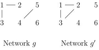
then networkg drawn in Figure 2 is a pairwise equilibrium network, where the links that can reduce costs the most do not exist in g.
1 2
3 4
5 6
7 8
Figure 2: Pairwise equilibrium network without the most valuable links
Given this outcome, one could easily imagine that in order to improve efficiency of the
equi-librium, public authorities may device policies that help the firms with the most valuable links to
improve the value of these links, say by providing additional resources. However the next example
shows that such a policy can lead to an equilibrium where the links that are formed are less valuable
13The authors use a sample of joint ventures taken from the Cooperative Agreements and Technology Indicators
database, a dataset that contains information on over 9000 alliances
and, as a result, the social welfare is lower. To simplify the construction of the example, we deal
with groups of links instead of groups of firms regarding the differences in the value of links. We
assume that because of the public policy, the value of the most valuable links is kv¯ instead of ¯v, with k > 1.
Example 3 Let N = {1, . . . ,6}, a = 490 7 , b =
5 7, c =
2 7, v
2 = 0.9, v1 = 0.8918244, and f =
89.752038. Suppose vi,j = v2 for ij ∈ {12,13,45}, vi,j = v1 for ij = 23, and vi,j = 0 for all other
links. Networkg in Figure 3 is the unique pairwise equilibrium network. Ifk = 1.000111, then, due to the public policy, network g′ in Figure 3 becomes the unique pairwise equilibrium network. We
can check that the total firms’ profit and the consumers’ surplus are higher in g′ than in g. Thus,
in this example, increasing the value of the most valuable links leads to an equilibrium where less
valuable links are formed, and social welfare is lower.
1 2
3 4
5
6
1 2
3 4
5
6
[image:19.612.217.376.394.474.2]Network g Network g′
Figure 3: Example of non-monotonicity
We now explain the intuition behind Example 3. First, the link 23, which is not the most
valuable, is not formed in g but is formed in g′. This result follows from the convexity of the
function φ with Vi(g): the increase in the value of the links 12 and 13 makes the formation of the
link 23 more attractive for firms 2 and 3. Second, one of most valuable links, the link 45 is formed
in g but is not formed in g′. This results from two opposing forces affecting the incentives to form
the link 45: (1) the value of the link 45 is higher, that makes this link more profitable; (2) the
lower than the second one.
Example 3 establishes that there are situations where an increase in the value of the most
profitable links by public authorities can be counterproductive since it leads to a decrease in the
social welfare. Thus it is important to have a precise idea concerning the properties of networks
that maximize the social welfare, and this is done next.
3.2
Efficient Networks
We begin with a proposition which establishes that in an efficient network if firm i has formed a link with firm j, then firm i has also formed a link with all firms that (a) have a lower marginal cost than j, and (b) whose collaboration with i has a higher value than the collaboration between
i and j.
Proposition 2 Let g be an efficient network that contains a link between firms i and j. If cj(g)≥
cj′(g) and vi,j ≤vi,j′, then there is a link between firms i and j′ in g.
The intuition behind Proposition 2 is as follows. First, suppose that firmj′ has a marginal cost
that is lower than j in g. Straightforward calculations show that if the linkij′ has the same value
as the link ij, then the addition of ij′ in g implies an increase in welfare that is higher than the
increase in welfare associated with the addition of the link ij in g−ij. Second, if the link ij′ has
a higher value than the link ij, then it is equivalent to a situation where the link ij′ has the same
value as the link ij, and a costless link is added to firmsiand j′. This link allows them to decrease
their marginal cost. Since the marginal cost of some firms decrease and the marginal cost of other
firms is unchanged, the welfare increases.
We now use Proposition 2 to identify the architectures of efficient networks in different situations.
Efficient networks in the framework of cost-reducing collaboration in a homogeneous Cournot game
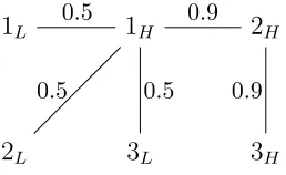
has been studied by Westbrock (Proposition 1, 2010) in situation where links have the same value.
1L 1H
2L 3L
2H
3H
0.5 0.9 0.9 0.5
[image:21.612.232.361.117.196.2]0.5
Figure 4: Relationship between flow degree and firms degree in efficient networks
framework are NSG. Here we extend the analysis to the I-O and H-L frameworks where links
have different values.
Corollary 4 Suppose that the assumptions of the I-O framework are satisfied. If g is a non-empty efficient network, then it is a NSG, or a 2-NSG, or a group-NSG, or a multi-NSG.
Corollary 5 Suppose that the assumptions of the H-L framework are satisfied. Ifg is a non-empty efficient network, then it is a NSG, or a group-NSG, or a multi-NSG. Moreover, if g[NH] =∅, then
g[NL] =∅.
We observe that in both the I-O and H-L frameworks, efficient networks are variations of NSG.
We now give the intuition behind this result. Consider Figure 4 in the H-L framework. The flow
degree of firm 1H is 2.4 and the flow degree of firm 2H is 1.8; the degree of 1H is 4 while the degree
of 2H is 2. By Proposition 2, network g cannot be an efficient network since firm 1H has to add a
link with firm 3H. The resulting network is a NSG which is a candidate to be an efficient network.
Since NSG are defined thanks to a property on degrees, this illustrates that the requirement on flow
degree for efficiency translates to a requirement on degrees.
The H-L framework provides an easy way to see the possibility of conflict between pairwise
equilibrium networks and efficient networks. In particular, in an efficient network, firms in NL will
not form links when it is not worthwhile for firms in NH to form links. By contrast, there are
Moreover, Lemma 1 (in Appendix) provides an interesting result for public authorities in the
H-L framework. Indeed, let g be a two-group-dominant pairwise equilibrium network. It results from Lemma 1 that social welfare can be increased if the R & D collaborative links formed by firm
i ∈NL with a subset of firms in AL⊂ NL in g are replaced by links formed by firm j ∈NH with
firms in AL⊂NL.
Conflict between pairwise equilibrium networks and efficient networks also arises in the I-O
framework, and public authorities can act to increase social welfare. For instance, consider a
group-dominant network such that the group-dominant group, as well as the set of isolated firms, contains firms
which belong to the two groups. It is easy to show that this network can be a pairwise equilibrium
network for some values of the parameters. The following proposition shows how social welfare
can be increased in this case. In this proposition, we denote by C(g) the dominant group in the group-dominant network g, and by Nk
IO(C(g)) the set of firms in the dominant group C(g) which
belong to group k,k = 1,2.
Proposition 3 Let g be a group-dominant network such that 0 < N1
IO(C(g)) < NIO1 and 0 <
N2
IO(C(g)) ≤ NIO2 . Wlog suppose NIO1 (g) ≥ NIO2 (g). Suppose i ∈ NIO1 \ NIO1 (C(g)) and j ∈
N2
IO(C(g)). Let g′ be a group-dominant network such that C(g′) = C(g)∪ {i} \ {j}. We have
W(g′)> W(g).
Moreover, when the size of the two groups are equal, that isN1
IO =NIO2 , we obtain the following
corollary.
Corollary 6 SupposeN1
IO =NIO2 . Letg be a group-dominant network such that0< NIO1 (g)< NIO1
and 0 < N2
IO(g) < NIO2 . Wlog suppose NIO1 (g) ≥ NIO2 (g). Let g′ be a a group-dominant network
such that N1
4
Results for a Larger Class of Oligopoly Games
In this section, we establish results for cases where the profit function satisfies some general
prop-erties. These properties are satisfied not only by our previous model, but also by models of
cost-reducing collaboration in differentiated (Cournot and Bertrand) oligopolies. In the following, we
assume that the gross profit function of firm i depends on its flow degree and the flow degree generated by the links in which firm i is not involved:
Πi(g) =σ(Vi(g),V(g−i)). (4)
We assume that the profit function of firm i is πi(g) = Πi(g)− |g(i)|f, where f > 0 is the cost of
link formation.
Broadly speaking, for a given value, v, two types of externality effects arise in our context: an externality across flow degree generated by the links in which firm i is involved, and an externality across flow degree generated by the links in which firmiis not involved. This motivates the following definitions.
Definition 3 The profit function,σ, is strictly convex in its first argument if for ally, σ(x+v, y)−
σ(x, y)> σ(x, y)−σ(x−v, y) for all x and v such that x≥v >0.
This definition means that for a given value of links, the higher the flow degree generated by
the links in which firm iis involved, the higher is the incentive of firm i to form an additional link. The next definition captures externality across flow degree of different firms.
Definition 4 The gross profit function,σ, is strictly sub-modular if for all x > v, and for ally′ > y
σ(x+v, y′)−σ(x, y′)< σ(x+v, y)−σ(x, y).
This definition means that for a given value of links, the higher the flow degree generated by the
link.
First, we state a proposition that provides necessary conditions for a pairwise equilibrium
net-work. This result complements the work of Goyal and Joshi (Proposition 3.1, p. 327, 2006), when
we allow heterogeneity in the values of the links. It is worth noting that our result highlights the
fact that a pairwise equilibrium network does not always contain the most valuable links.
Proposition 4 Suppose that the gross payoff function is given by (4) where σ is strictly increasing and strictly convex in its first argument, and sub-modular. Let g be a pairwise equilibrium network, with ij ∈g and ij′ ∈/ g. Then, V
j(g)>Vj′(g) or vi,j > vi,j′.
Proposition 4 states that it is not possible to have a situation where simultaneously (a) two unlinked firms i′, j′ have a cost competitive advantage, and (b) the link between them is more
valuable than the links that have already been formed.
We now provide two examples of more general oligopoly models that satisfy the conditions of
Proposition 4. For both examples, we assume that the cost function is given by equation 1.
Example 4 Differentiated Cournot Oligopoly. Suppose each firmifaces the following linear inverse demand function: pi = α −qi − β
P
j6=iqj, where pi is the price of the product sold by firm
i, α > 0, and β ∈ (0,1). In the Cournot equilibrium, the gross profit for firm i is given by: Πd
i(g) =θ(Vi(g),V(g−i)) = (a1+a2Vi(g)−a3 V(g−i))2, with a1,a2, and a3 as positive parameters.15
Moreover, to ensure that each firm produces a strictly positive quantity in equilibrium, assume that
a1 > a3V(g−i) for all V(g−i).
Example 5 Differentiated Bertrand Oligopoly. Suppose the demand function is similar to those given in Example 4. In the Bertrand equilibrium, the gross profit for firm i is given by: ΠB
i (g) =
θi(Vi(g),V(g−i)) =λ(a1 +a2Vi(g)−a3V(g−i))2, with λ, a1, a2, and a3 as positive parameters.
It is worth noting that Example 3 was based on the fact that the profit function is convex in
its first argument and sub-modular. It follows that when σ satisfies these two properties, as in Examples 4 and 5, a policy designed to increase the value of the most valuable links may lead
to equilibrium networks that do not have them, while equilibrium networks obtained without this
policy may have these links in equilibrium. This suggests caution regarding public policy aimed at
promoting R&D collaboration.
To study efficient networks, we need an additional condition on σ regarding the role played by the links of other firms in the profit function of each firm.
Definition 5 The gross profit function, σ, is strictly convex in its second argument if for all x,
v >0, σ(x, y+v)−σ(x, y)> σ(x, y)−σ(x, y−v) for all y.
It is worth noting that Examples 4 and 5 satisfy this convexity property. Moreover, for efficient
networks we also need two simple additional monotonicity preserving type assumptions, the first
one on the consumer surplus part (Property PCS), the second one on the social welfare (Property
PW).
Property PCS:Let the marginal cost of firmsℓandℓ′ be lower than the marginal cost of firms
j and j′ respectively. Suppose that first we decrease the marginal cost of j and j′ by v, then we
decrease the marginal cost of ℓ and ℓ′ byv. Then, the change in the consumer surplus is higher in
the second case than in the first case.
Note that Property PCS is satisfied by the demand functions presented in this paper, for cost
function given by (1).
Property PW implies that for a given network, it is always efficient to increase the value of the
links formed by the firms.
The next proposition establishes that if (a) two firmsj andj′ have higher flow degree than firms
i and i′ respectively, and (b) the value of the link jj′ is sufficiently high with regard to those ofii′,
then in an efficient network firms j and j′ are linked when firmsi and i′ are linked.
Proposition 5 Let g be a non-empty efficient network with Vi(g) ≤ Vj(g) and Vi′(g) ≤ Vj′(g).
Suppose σ is strictly convex in its first and second arguments, σ is sub-modular, and the properties PCS and PW are satisfied. If there exists a link between firms i and i′ and v
i,i′ ≤ vj,j′, then there
exists a link between firms j and j′.
Note that if we set j =i, then we can obtain a result in line with Proposition 2.
Proposition 5 shows that two elements play a role in the existence of a link between two firmsi
and j in an efficient network: the first one is the flow of knowledge that accrues to these two firms due to their collaborations with other firms in the network, relative to the flow of knowledge that
accrues to other linked firms; the second one is the value of the link between iand j relative to the value of the existing links.
5
Concluding remarks
This paper extends the work of Goyal and Joshi (2003) on collaborative R&D network formation
by assuming that cost reducing innovations between pairs of firms are heterogeneous. Clearly if
every link takes a different value, the model has many degrees of freedom and can easily generate a
rich set of results. Hence after providing a necessary condition to check for a pairwise equilibrium
network or an efficient network when all links can have different values, we limit the set of values
frameworks, the I-O and H-L frameworks. Not surprisingly, we find that results of Goyal and Joshi
(2003), Westbrock (2010) and Billand et al. (2015) as special cases, since all links have the same
value in these models. We then provide results for a larger class of games like differentiated Cournot
and Bertrand games.
An interesting result regarding public policy is that when this policy is used to increase the value
of links having the highest value, this policy can lower welfare, given that some of the most valuable
links may disapear in equilibrium. This result highlights the difference between our framework and a
framework without links value heterogeneity, that isvi,j = 1 for all firmsi, j, but with heterogeneous
costs of forming links.16 Recall that the result in Example 2 uses the fact that when we make the
most valuable links better some firms that have formed these links have strong incentives to form
additional links, including less valuable ones. Consequently, if some firms add links, then other firms
may remove some of their links, including the most valuable links. Hence, due to the substitution of
less valuable links for some of the most valuable ones, public policy aimed at increasing the worth
of the most valuable links may lead to welfare loss. Observe that links value heterogeneity is crucial
for this type of non-monotonicity result. Moreover, this result cannot be obtained in a framework
where the costs of forming links are heterogeneous. Indeed, in that case, firms that benefit from a
policy subsidizing the cheapest existing links, do not have any incentive to form additional links,
and the mechanism that leads to a welfare loss in the value heterogeneity framework cannot occur
in the cost heterogeneity framework.
In our model, we have assumed that when two firms collaborate and innovate, each of them benefits
in an identical manner from the innovation. In practice this may not be so. As a final point, we
now illustrate what happens if we relax this assumption. Suppose that when the link ij is added to network g, the marginal cost of firmiis reduced by τi and the marginal cost of firmj is reduced by
τj where τi 6=τj. Obviously, if τi is sufficiently high relative to τj, then firm j will never accept to 16In the theoretical literature on network formation, several papers examine this type of heterogeneity (see for
form the link with i. Indeed, link ij improves the competitiveness of firm iso much more than the competitiveness of firm j that the latter firm will lower its profit by forming the link ij. Due to this mechanism, firms have an incentive to form links only with other firms that will not increase their
competitiveness by a too substantial amount. Therefore, we can obtain a “tyranny of the weakest”
situation, that is a situation in which the least able firms to take advantage of R&D collaboration
form links with each other, leaving out the most able firms. A detailed examination of this issue is
left for future research.
References
[1] P. Billand, C. Bravard, and S. Sarangi. Strict Nash networks and partner heterogeneity.
International Journal of Game Theory, 40(3):515–525, August 2011.
[2] P. Billand, C. Bravard, and S. Sarangi. Modeling resource flow asymmetries using condensation
networks. Social Choice and Welfare, 41(3):537–549, 2013.
[3] Billand P., Bravard C., Durieu J., Sarangi S. Efficient networks for a class of games with global
spillovers. Journal of Mathematical Economics, 61: 203–210, 2015.
[4] R. Blundell, R. Griffith, and J. van Reenen. Market share, market value and innovation in a
panel of british manufacturing firms. Review of Economic Studies, 66(3):529–554, 1999.
[5] U. Blum, C. Fuhrmeister, P. Marek, and M. Titze. R&D collaborations and the role of
prox-imity. Regional Studies, 51(12): 1761–1773, 2017
[6] A. Galeotti, S. Goyal, and J. Kamphorst. Network formation with heteregeneous players.
Games and Economic Behavior, 54(2):353–372, 2005.
[7] B. Gomes-Casseres, J. Hagedoorn, and A. Jaffe. Do alliances promote knowledge flows? Journal
[8] S. Goyal and S. Joshi. Networks of collaboration in oligopoly. Games and Economic Behavior,
43(1):57–85, 2003.
[9] S. Goyal and S. Joshi. Unequal connections. International Journal of Game Theory, 34(3):319–
349, 2006.
[10] S. Goyal and J.L Moraga-Gonzalez. R&D networks. The RAND Journal of Economics,
32(4):686–707, 2001.
[11] S. Goyal, J.L. Moraga-Gonzalez, and A. Konovalov. Hybrid R&D. Journal of the European
Economic Association, 6(6):1309–1338, December 2008.
[12] J. Hagedoorn. Inter-firm R&D partnerships: An overview of major trends and patterns since
1960. Research Policy, 31(4):477–492, 2002.
[13] M. D. K¨onig, S. Battiston, M. Napoletano, and F. Schweitzer. The efficiency and stability of
R&D networks. Games and Economic Behavior, 75(2):694–713, 2012.
[14] M. D. K¨onig, C. J. Tessone, and Y. Zenou. Nestedness in networks: A theoretical model and
some applications. Theoretical Economics, 9(3):695–752, 2014.
[15] N.V.R. Mahadev, and U.N. Peled. Threshold graphs and related topics. North Holland,
Amsterdam, 1995.
[16] D.C. Mowery, J.E. Oxley, B.S. Silverman. Technological overlap and interfirm cooperation:
implications for the resource-based view of the firm. Research Policy, 27(5):507–523, 1998.
[17] D. Persitz. Core-periphery R&D collaboration networks. Working paper, 2014.
[18] W.W. Powell, D.R. White, K.W. Koput, and J. Owen-Smith. Network dynamics and field
evo-lution: The growth of interorganizational collaboration in the life sciences. American Journal
[19] M.V. Tomasello, M. Napoletano, A. Garas, F.Schweitzer. The rise and fall of R&D networks.
Industrial and Corporate Change, 2016.
[20] N. Vonortas, K. Okamura. Research Partners. International Journal of Technology
Manage-ment, 46(3/4):280–306, 2009.
[21] N. Vonortas, K. Okamura. Network Structure and Robustness: Lessons for Research
Pro-gramme Design. Economics of Innovation and New Technology, 46(3/4):280–306, 2013.
[22] N. Vonortas, L. Zirulia. Strategic Technology Alliances and Networks. Economics of Innovation
and New Technology, 22(4):392–411, 2015.
[23] B. Westbrock. Natural concentration in industrial research collaboration. The RAND Journal
of Economics, 41(2):351371, 2010.
Appendix
Appendix A. Definitions
Nested Split Graph(Mahadev and Peled, 1995) Letgbe a network whose distinct positive degrees are δ1 < . . . < δm, and letδ0 = 0 (even if no firm of degree 0 exists). LetDk(g) ={i∈N :|gi|=δk}
for k ∈ {0, . . . m}. The sequence D0(g), . . . , Dm(g) is called the degree partition of G. In a nested
split graph (NSG) g, we have for each firm i∈Dℓ(g),ℓ ∈ {1, . . . , m},
g(i) =
Sℓ
j=1Dm+1−j(g), if ℓ= 1, . . . , m
2
,
Sℓ
j=1Dm+1−j(g)\ {i}, if ℓ=
m
2
Appendix B. Homogeneous Cournot Game
In Appendix B and C, we let ∆1ϕ(Vi(g),V(g−i);vij) =ϕ(Vi(g) +vi,j,V(g−i))−ϕ(Vi(g),V(g−i)) and
∆2ϕ(Vi(g), V(g−i);vℓ,j) =ϕ(Vi(g),V(g−i) +vℓ,j)−ϕ(Vi(g),V(g−i)). Moreover, we let Sϕ(x, y, h) = ϕ(x+h,y)−ϕ(x,y)
h .
First, note that in the homogeneous Cournot game ∆1ϕ is increasing in its first argument and
decreasing in its second argument.
Proof of Proposition 1 First, note that since ϕ(x, y) = (a+bx−cy)2, we have:
Sϕ(x, y;h) = ¯ϕ′1(x, y;h).
Second, since g is a pairwise equilibrium network where player i and j have formed a link, we have
∆1ϕ(Vi(g)−vij,V(g−i);vij)≥f.
We now prove successively the two parts of the proposition
1. Suppose that
v vi,j
≤ ϕ¯
′
1(Vi(g),V(g−i);vi,j)
¯
ϕ′
1(Vi(g)−v,V(g−i);v)
.
Then, we have
v vi,j
≤ Sϕ(Vi(g),V−i(g);vi,j)
Sϕ(Vi(g)−v,V(g−i);v)
,
and so ∆1ϕ(Vi(g),V(g−i);vi,j)≥∆1ϕ(Vi(g)−v,V(g−i);v). It follows that ∆1ϕ(Vi(g),V(g−i);
vi,j)≥f, and firmi has an incentive to form a link with firm j. By using similar arguments,
we obtain that firm j has an incentive to form a link with firm i. Consequently, g is not a pairwise equilibrium, a contradiction.
2. We assume that firmsi, j ∈N \ {i′, j′}are linked in g, andv
To introduce a contradiction, we assume that i′j′ 6∈ g. Since ¯ϕ′
1(Vi′(g),V(g−i′);vi′,j′) ≥
¯
ϕ′1(Vi′(g),V(g−i′)−v;v), we have: Sϕ(Vi′(g),V(g−i′);vi′,j′)≥Sϕ(Vi′(g),V(g−i′)−v;v).
There-fore, we have vSϕ(Vi′(g),V(g−i′);vi′,j′) ≥ vSϕ(Vi′(g),V(g−i′)−v;v). Since vi′,j′ ≥ v, we have
vi′,j′Sϕ(Vi′(g),V(g−i′);vi′,j′))≥vSϕ(Vi′(g),V(g−i′);vi′,j′)). Consequently, we have ∆1ϕ(Vi′(g), V(g−i′);vi′,j′) ≥ ∆1ϕ(Vi′(g),V(g−i′)−v;v) = ∆1ϕ(Vi(g)−v,V(g−i);v) ≥ 0. It follows that
firmi′ has an incentive to form a link withj′ ing. By using similar arguments, we obtain that
j′ has an incentive to form a link with i′ in g. Consequently, g is not a pairwise equilibrium
network, a contradiction.
Finally, by construction all the pairs in (V, v′;V(g
−i′))≥ lead to marginal net profits higher
or equal to ∆1ϕ(V,V(g−i′);v′). Since we have (Vi′(g), vi′,j′) in (V, v′;V(g−i′))≥, it follows that
firm i′ has an incentive to form a link with j′. Since V
j′(g) ≥ Vi′(g) and V(g−j′) ≤ V(g−i′),
we have ∆1ϕ(Vj′(g),V(g−j′);vi′,j′) ≥ ∆1ϕ(Vi′(g),V(g−i′);vi′,j′). Consequently, firms i′ and j′
have an incentive to form a link in g.
Proof of Corollary 1 We prove successively the two parts of the proposition.
1. Suppose that vi,j ≥v. Then, we have
¯
ϕ′
1(Vi(g),V(g−i);vi,j)
¯
ϕ′
1(Vi(g)−v,V(g−i);v)
= 1 + b(vi,j+v)
2(a+bVi(g)−cV(g−i))−bv
>1≥ v
vi,j
,
because b >0 and 2a+ 2bVi(g)−2cV(g−i)−bv > 0. The result follows by Proposition 1.1.
2. Suppose thatVj′ ≥ Vi′ ≥ Vi and vi′,j′ ≥v. We are in special case of Proposition 1.2. We have
∆1ϕ(Vi′(g),V(g−i′);vi′,j′) = 2bvi′,j′(a+bVi′(g)−cV(g−i′)) +b2v2i′,j′ ≥ 2bv(a+bVi(g)−cV(g−i))−b2v2
= ∆1ϕ(Vi(g)−v,V(g−i);v)
because Vi′(g)≥ Vi(g), V(g−i′)≤ V(g−i), andvi′,j′ ≥v.
It follows that firm i(resp. j) has an incentive to form a link with j (resp. i). Consequently,
g is not a pairwise equilibrium network, a contradiction.
Proof of Corollary 2. Let g be a non-empty pairwise stable network. First, we establish that g
is a group-dominant network, or a 2-group-dominant network, or a 2|2-hierarchical network, or a
1|2-hierarchical network. By Corollary 1.1, if firm i ∈ Nk
IO, k ∈ {1,2}, is involved in a link with
firm j ∈Nk
IO ing, then i has an incentive to form a link with all other firms inNIOk . Moreover, by
Corollary 1.1 and the fact that vI > vO, if firm i∈Nk
IO,k ∈ {1,2}, is involved in a link with a firm
j ∈ N−k
IO, then i has an incentive to form a link with all firms in N. It follows that (i) two firms
which belong to the same group and have formed links must be linked together, (ii) two firms that have formed inter-groups links must be linked together. Let us now establish successively the three
parts of the proposition.
1. Letg be a 2-group-dominant network. Moreover, suppose that|N1
IO(g)| ≤ |NIO2 (g)|. We show
that each component consists of firms which belong to the same group Nk
IO. To introduce a
contradiction, suppose that there exists a link between firm i∈N1
IO and firm j ∈NIO2 . Since
there are two components there exists firm i′ which has formed a link in g and which is not
connected with i and j. Wlog, we suppose that i′ ∈ N1
IO. By Corollary 1.1, firms i and i′
have an incentive to form a link. Consequently, g is not a pairwise equilibrium network, a contradiction.
2. Let g be a 2|2-hierarchical network. First, note that if firm i ∈ Nk
IO has formed a link with
firm j′ ∈ N−k
IO, then i has an incentive to form a link with all firms in N by Corollary 1.1.
Moreover, by Corollary 1.1, if firm i has formed a link with firm j ∈ Nk
IO, then i has an
incentive to form a link with all firms in Nk
3. Let g be a 1|2-hierarchical network where some firms in Nk
IO(g) have formed links with all
other firms in NIO−k(g). We use the same type of arguments as in point 2.
Proof of Corollary 3. Let g be a non-empty pairwise stable network. First, we establish that
g is a group-dominant network, or a 2-group-dominant network, or a 1|(1,1)-hierarchical network, or a 1|2-hierarchical network. Consider firm i ∈NH that has formed a link with firm j ∈NL. By
Corollary 1.1 and the fact that vH > vM, firmi has an incentive to form a link with all firms inN.
Consider firm i ∈NH that has formed a link with i′ ∈ NH and has formed no links with firms in
NL. Then, by Corollary 1.1 firm ihas formed a link with all firms inNH(g). Consider firm j ∈NL
that has formed a link with j′ ∈ NL. Then, by Corollary 1.1, firm i has formed a link with every
firm j′ ∈NL(g). The result follows. Moreover, these arguments allow to prove the last part of the
proposition. We now establish successively the two first parts of the corollary.
1. Let g be a 2-group-dominant network. Then there are two components C1 and C2. Consider
that component C1 contains only firms NH and component C2 contains only firms in NL. To
introduce a contradiction suppose that C1 contains a firm i ∈ Nk and C2 contains j ∈ Nk,
then by Corollary 1.1, i and j are linked in g. Let us now show that |NH(g)| < |NL(g)|.
To introduce a contradiction suppose that |NH(g)| ≥ |NL(g)|. We know that vH > vL. We
have for firms i∈ NH(g) and i′ ∈NL(g), V
i(g)≥ Vi′(g). By Corollary 1.1 and the fact that
vM > vL, it follows that firm i′ has an incentive to form a link with firm i. Moreover by
Corollary 1.2 and the fact that vM > vL, firm i has an incentive to form a link with firm i′.
It follows that i and i′ are linked in g, a contradiction.
2. Letg be a 1|2-hierarchical network. Since firms inNL(g) have an incentive to form links with
all firms, we obtain the result. We now establish that|NH(g)\NHL(g)|< NL(g). To introduce
a contradiction, suppose that |NH(g)\NHL(g)| ≥NL(g). Then, for firmsi∈NH(g)\NHL(g)
andj ∈NL(g) , we haveV