Structure and properties of some triangular lattice materials

STRUCTURE AND PROPERTIES OF SOME TRIANGULAR

LATTICE MATERIALS

Lewis James Downie

A Thesis Submitted for the Degree of PhD

at the

University of St Andrews

2014

Full metadata for this item is available in

St Andrews Research Repository

at:

http://research-repository.st-andrews.ac.uk/

Please use this identifier to cite or link to this item:

http://hdl.handle.net/10023/4423

Structure and Properties of Some Triangular Lattice

Materials

Lewis James Downie

This thesis is submitted in partial fulfilment for the degree of

PhD

at the

i

1. Candidate’s declarations:

I, Lewis James Downie, hereby certify that this thesis, which is approximately 38,000 words in length, has been written by me, that it is the record of work carried out by me and that it has not been submitted in any previous application for a higher degree.

I was admitted as a research student in March, 2010 and as a candidate for the degree of PhD in January, 2011; the higher study for which this is a record was carried out in the University of St Andrews between 2010 and 2013.

Date …… signature of candidate ………

2. Supervisor’s declaration:

I hereby certify that the candidate has fulfilled the conditions of the Resolution and Regulations appropriate for the degree of PhD in the University of St Andrews and that the candidate is qualified to submit this thesis in application for that degree.

Date …… signature of supervisor ………

3. Permission for electronic publication: (to be signed by both candidate and supervisor) In submitting this thesis to the University of St Andrews I understand that I am giving permission for it to be made available for use in accordance with the regulations of the University Library for the time being in force, subject to any copyright vested in the work not being affected thereby. I also understand that the title and the abstract will be published, and that a copy of the work may be made and supplied to any bona fide library or research worker, that my thesis will be

electronically accessible for personal or research use unless exempt by award of an embargo as requested below, and that the library has the right to migrate my thesis into new electronic forms as required to ensure continued access to the thesis. I have obtained any third-party copyright permissions that may be required in order to allow such access and migration, or have requested the appropriate embargo below.

The following is an agreed request by candidate and supervisor regarding the electronic publication of this thesis:

Embargo on both [all or part] of printed copy and electronic copy for the same fixed period of 2 years (maximum five) on the following ground(s):

publication would preclude future publication;

Date …… signature of candidate …… signature of supervisor ………

ii

Abstract

This thesis is concerned with the study of two families of materials which contain magnetically frustrated triangular lattices. Each material is concerned with a different use; the first, analogues of YMnO3, is from a family of materials called multiferroics, the second, A2MCu3F12 (where A = Rb1+, Cs1+, M = Zr4+, Sn4+, Ti4+, Hf4+), are materials which are of interest due to their potentially unusual magnetic properties deriving from a highly frustrated Cu2+-based kagome lattice.

YFeO3, YbFeO3 and InFeO3 have been synthesised as their hexagonal polymorphs. YFeO3 and YbFeO3 have been studied in depth by neutron powder diffraction, A.C. impedance spectroscopy, Mössbauer spectroscopy and magnetometry. It was found that YFeO3 and YbFeO3 are structurally similar to hexagonal YMnO3 but there is evidence for a subtle phase separation in each case. Low temperature magnetic properties are also reported, and subtle correlations between the structural, electrical and magnetic properties of these materials have been found. InFeO3 was found to adopt a higher symmetry and is structurally similar to the high temperature phase of YMnO3. TbInO3 and DyInO3 have also been synthesised and studied at various temperatures. The phase behaviour of TbInO3 was analysed in detail using neutron powder diffraction and internal structural changes versus temperature were mapped out – there is also evidence for a subtle isosymmetric phase transition. Neither DyInO3 nor TbInO3 show long-range magnetic order between 2 and 300 K, or any signs of ferroelectricity at room temperature.

iii

Acknowledgements

On completing this PhD thesis I would like to thank Prof. Phil Lightfoot for his generous supervision throughout the past three and a half years. The opportunity, and since then the calm and considered mentoring, has been invaluable in my development as a chemist.

Lesser, but still important, is my thanks to all the other academics and researchers that have helped me through my work with their specialist skills and understanding. Even though some results have not made it into this thesis they have still been essential in developing understanding and identifying future pathways for research. In the School of Chemistry: Dr F. D. Morrison, Prof. A. M. Z. Slawin, Prof. W. Zhou and Mrs S. Williamson have all helped in the acquisition of results and their analysis. Other specialists from further afield have also contributed their knowledge or helped me with new techniques or equipment. These include

Drs W. Kockelmann, A. Daoud-Aladine and D.A. Keen of ISIS pulsed neutron and muon source, Prof. C. C. Tang and Drs Stephen Thompson and J. E. Parker of Diamond Light Source. Outside of central facilities support was found from Dr S. D. Forder, who ran a number of critical Mössbauer spectra, Dr M. A. de Vries, who has been a key collaborator in the collection and analysis of magnetic data, Dr A. F. Kusmartseva who helped with early magnetic measurements and Dr A. L. Goodwin who introduced me to pair distribution function analysis.

Prof. S. Parsons was more than helpful with the collection of some particularly complex data and I am particularly indebted for his time and efforts.

I am very grateful for the warm hospitality and specialist instruction I received at the department of chemistry, Moscow State University from Prof. V. A. Dolgikh, Drs E. I. Ardashnikova, P. S. Berdonosov and D. O. Charkin. I am also appreciative of the further help I received from Prof. A. N. Vasiliev and Mr A. Golovanov of the low temperature physics department.

Outside of research I have received a great deal of support, patience and understanding from my partner, Laura Mitchell. I have also made many new friends within the chemistry department – and outside of it – who have been more than supportive both in terms of work and diversionary activities. Old friends have also supplied welcome encouragement. I would also like to thank my parents, James Downie and Margaret Downie,

iv

Contents

1

Introduction

1

1.1 Multiferroics 2

1.1.1 Magnetism 2

1.1.1.1 Variations of magnetism with temperature 3

1.1.1.2 Variations of magnetism with size 6

1.1.2 Ferroelectricity 6

1.1.2.1 Origins of ferroelectricity 6

1.1.3 Multiferroic materials 8

1.1.4 Hexagonal rare-earth manganites 9

1.1.4.1 Magnetism in MMnO3 10

1.1.4.2 Ferroelectricity in MMnO3 11

1.1.4.3 The magnetoelectric effect in MMnO3 12

1.2 Quantum spin liquids 12

1.2.1 Possible quantum spin liquids 14

1.2.1.1 Herbertsmithite 15

1.2.1.2 Kapellasite 15

1.2.1.3 DQVOF 16

1.2.2 The A2MCu3F12 family 17

1.3 Aims 19

2

Experimental techniques

23

2.1 Diffraction 24

2.1.1 Diffraction in practice 27

2.1.1.1 Structural model refinement 29

2.1.2 Synchrotron X-ray diffraction 30

2.1.3 Neutron diffraction 31

2.1.3.1 Neutrons and the determination of magnetic structure 31

2.2 Magnetometry 32

2.2.1 SQUID magnetometer measurements 32

2.2.2 VSM measurements 33

2.3 Electrical measurements 33

2.4 Mössbauer spectroscopy 35

3

Crystallographic and magnetic studies of the novel

kagome compounds A

TiCu

F

(where A = Rb, Cs)

37

3.1 Experimental 38

3.1.1 Synthesis of A2TiF6 38

3.1.2 Synthesis of A2TiCu3F12 38

3.1.3 Analysis techniques 39

3.2 Crystallography of Cs2TiCu3F12 40

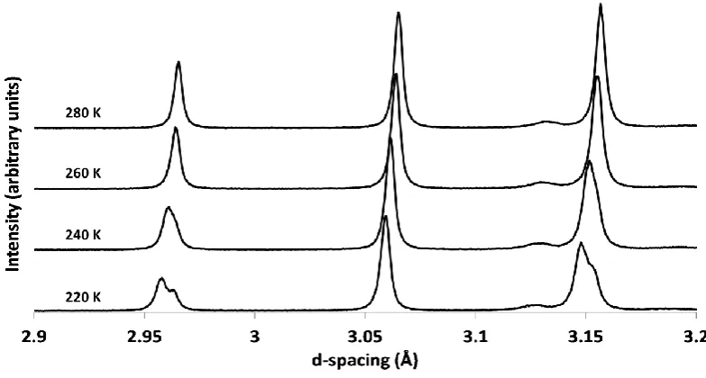
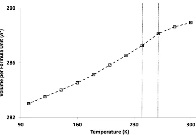
3.2.1 Variable temperature studies of Cs2TiCu3F12 by powder diffraction 41

3.2.2 Single crystal X-ray diffraction studies of Cs2TiCu3F12 50

3.2.3 Cs2TiCu3F12: a material with crystallite size dependent phase

transitions 53

3.3 Crystallography of Rb2TiCu3F12 56

3.4 Magnetic properties of Cs2TiCu3F12 61

3.5 Properties of Rb2TiCu3F12 65

v

4

Studies of Rb

SnCu

F

– a kagome compound with

re-entrant structural phase transition

71

4.1 Experimental 73

4.1.1 Synthesis of Rb2SnCu3F12 73

4.1.2 Analytical techniques 73

4.2 SXPD studies of Rb2SnCu3F12 74

4.3 NPD studies of Rb2SnCu3F12 81

4.4 Single crystal studies of Rb2SnCu3F12 84

4.5 Structurally re-entrant transitions 87

4.6 Conclusions 87

5

Crystallographic studies of Cs

Rb

SnCu

F

(where

x = 0, 0.5, 1.0, 1.5)

89

5.1 Experimental 90

5.1.1 Synthesis of Cs2-xRbxSnCu3F12 90

5.1.2 Analysis techniques 91

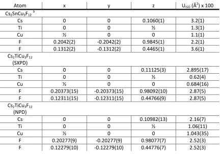
5.2 Crystallography of Cs2SnCu3F12 91

5.3 Crystallography of Cs2-xRbxSnCu3F12 97

5.3.1 Cs1.5Rb0.5SnCu3F12 98

5.3.2 CsRbSnCu3F12 100

5.3.3 Cs0.5Rb1.5SnCu3F12 102

5.4 Structural trends in the A2SnCu3F12 solid solution 106

5.5 Magnetic properties of Cs2SnCu3F12 powder 108

5.6 Conclusions 112

6

Structural, electrical and magnetic properties of the

hexagonal ferrites, MFeO

(where M = Y, Yb or In)

113

6.1 Experimental 114

6.1.1 Synthesis of YFeO3 and YbFeO3 114

6.1.2 Synthesis of InFeO3 115

6.1.3 Analytical techniques 115

6.2 Results 116

6.2.1 Crystallography and structure of MFeO3 116

6.2.2 Electrical studies of MFeO3 122

6.2.3 Magnetic properties of MFeO3 122

6.2.4 Mössbauer studies of MFeO3 126

6.3 Discussion 128

6.3.1 A two-phase model 128

6.3.2 Magnetic-electrical-structural link 131

6.3.3 Low temperature magnetic structure 134

6.4 Conclusion 137

7

Studies of MInO

(where M = Dy, Tb)

139

7.1 Experimental 140

7.1.1 Synthesis of DyInO3 and TbInO3 140

7.1.2 Analytical techniques 140

7.2 Structural studies of MInO3 141

7.3 Magnetic and electrical behaviour of MInO3 152

7.4 Conclusions 155

vi

8.1 Analogues of YMnO3 158

8.2 Materials from the family A2MCu3F12 159

8.3 Future work 160

---

Selected Appendices

---

A.3.2.1 Lattice parameters vs. temperature for Cs2TiCu3F12 161

A.3.3 Comparison of SCXRD and NPD parameters for Rb2TiCu3F12 / Lattice

parameters vs. temperature for Rb2TiCu3F12 162

A.3.4 Kapton data subtraction 165

A.4.2 Lattice parameters vs. temperature for Rb2SnCu3F12 – synchrotron /

Lattice parameters vs. temperature for Rb2SnCu3F12 - neutron 166

A.5.2 Lattice parameters vs. temperature for Cs2SnCu3F12 – neutron /

Lattice parameters vs. temperature for Cs2SnCu3F12 – synchrotron 173

A.5.3.1 Lattice parameters vs. temperature for Cs1.5Rb0.5SnCu3F12 177

A.5.3.2 Lattice parameters vs. temperature for CsRbSnCu3F12 179

A.5.3.3 Lattice parameters vs. temperature for Cs0.5Rb1.5SnCu3F12 181

A.5.4 Lattice parameters of the series Cs2-xRbxSnCu3F12 in monoclinic

setting 183

A.6.2.1 Lattice parameters vs. temperature for YFeO3 / Lattice parameters

vs. temperature for YbFeO3 185

A.6.3.3 Magnetic fits for YFeO3 / Magnetic fits for YbFeO3 188

A.7.2 Lattice parameters vs. temperature for DyInO3 / Lattice parameters

1

2

This thesis is concerned with observing the – mostly structural – effects of substituting ions in two functional materials of current academic interest. Both materials contain magnetic lattices that are based upon a triangular motif, which is synonymous with magnetic frustration. However, the materials have very different characteristics – one looks to avoid magnetic order and thus enter into an exotic magnetic state called a “quantum spin liquid” whereas the other looks to magnetically order despite the frustration. The former, the A2MCu3F12 family, is based upon a highly frustrated Cu2+ kagome lattice which has previously been shown to encourage novel and exotic magnetic behaviours. The latter, YMnO3, is based upon a triangular Mn3+ lattice but has been shown to undergo long-range magnetic order; coupled with the ferroelectric properties of this material this yields a material called a “multiferroic” in which two or more forms of order are present within the material simultaneously. In this discussion it is advantageous to discuss the types of order possible in the two materials first.

1.1

Multiferroics

A multiferroic is a material that combines two types of ordering from the classes ferroelectric, magnetic and ferroelastic1. The term is principally associated with materials that combine both magnetic and ferroelectric ordering (even in cases of antiferromagnetic ordering) and so these form the focus of this introduction.2 Ferroelastic materials are those which show a spontaneous deformation. Magnetoelectric multiferroics are of particular interest as there is the possibility of a linkage between the magnetic and ferroelectric ordering (the magnetoelectric effect). This linkage is usually found in materials where the source of magnetism and ferroelectricity are the same and are called type-II multiferroics. The preceding type-I multiferroics generally have different sources of magnetism and ferroelectricity and thus have only a weak, if observable, linkage.2 Such cross interference is useful in areas such as data storage as one could write electrically and read magnetically, for example.3

It is important to have a basic understanding of ferroelectric and magnetic ordering in order to compare and contrast their requirements and to understand their measurement.

1.1.1 Magnetism

3

If both M and H are known then it is possible to calculate the magnetic susceptibility of the material (Equation 1.1)

1.1

From this the molar susceptibility, χm, can be acquired leading to a comparative value for a number of different materials. However, this is comparative only if measured in the same conditions as this value is found to change with temperature. Such changes also betray the existence of more than the two behaviours previously alluded to.

1.1.1.1 Variations of magnetism with temperature

For diamagnetic materials there is no variation of χ with temperature as its origin is not subject to thermal disorder. Paramagnetism is subject to variation with temperature as its positive interaction is due to alignment of the unpaired electron spins with H. As the temperature is increased the tendency to align with H is reduced due to increasing thermal disorder. Most paramagnetic materials approximately follow the Curie law with varying temperature:

1.2

(where C = Curie constant and T = Temperature)

A modification of the Curie law which often provides for a better fit is the Curie-Weiss law which takes into account the Weiss constant, TCW, of the material5.

1.3

The above formulae suggest the type of behaviour shown in Figure 1.1.

C is related to the magnetic moment, μ (in Bohr magnetons), by equation 1.4.

√ 1.4

The magnetic moment can be compared to that expected for individual ions for transition metals (Equation 1.5) and lanthanides (Equation 1.6).

√ 1.5

(where S = spin state of the ion)

√ (

) 1.6

4

Figure 1.1: Qualitative behaviour for χ of a paramagnet as a function of temperature.

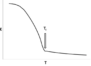
As suggested there are variations to paramagnetic behaviour6. On cooling, ferromagnetic materials shows a paramagnetic behaviour until a certain temperature (the Curie temperature, TC) at which point χ increases markedly (Figure 1.2).

5

The rapid increase in χ at TC is due to the spins within the sample aligning with each other and the external field, H. For a paramagnetic sample the spins do not align with each other but align with the magnetic field independently; a process which leads to less overall alignment. Such a clear distinction exists between the two possible behaviours as at TC the thermal energy is enough to overcome the spin ordering energy.

Ferromagnetic materials can show a hysteresis loop in their spontaneous magnetisation; they can retain a magnetic polarisation that has been previously applied to them. It is this retention of a residual magnetic field which is exploited for data storage. Different ferromagnetic materials have different hysteretic behaviours and so lend themselves to different applications.

Another exception to the two main regimes is antiferromagnetism. In this case the material appears as paramagnetic at elevated temperature but below a critical temperature it is found that χ begins to decrease (Figure 1.3). The transition temperature (the Néel point, TN) signals the point at which spins begin to order internally but instead of aligning in the same direction, as for ferromagnetism, they align in opposite directions. This ordering leads to the magnetic moments cancelling out.

Figure 1.3: Qualitative behaviour of χ vs. T for an antiferromagnetic sample.

6

Figure 1.4: Different magnetic orders on a one dimensional line of spins; from top: ferromagnetism, antiferromagnetism, ferrimagnetism, canted ferromagnetism.

1.1.1.2 Variations of magnetism with size

In the bulk, the above effects are usually found but on reducing particle size unusual effects can occur. One of these effects is superparamagnetism. In this effect the particle size is so small that its entirety exists as one ferromagnetic or ferrimagnetic magnetic domain. The net magnetic moment is constantly changing and thus gives the appearance of zero moment. On the application of a magnetic field, however, there is the appearance of a larger magnetic field than would be given for a purely paramagnetic system. This is because there is a slight ferro/ferrimagnetic character to the system. On cooling, the time required for the domain to change direction increases and below a certain temperature, the blocking temperature, the systems appears as a ferro/ferrimagnetic system.7

1.1.2 Ferroelectricity

Ferroelectricity has many parallels with magnetism. Most inorganic insulators are found to be from a class of materials called dielectrics. This class is characterised by an electrical polarisation across the material when a potential difference is applied, but application of that potential difference does not lead to long-range movement of electrons or ions. The polarisation also disappears when the potential difference is removed; this is in analogy to a paramagnetic substance. This analogy is continued by the occurrence of a type of dielectric, a ferroelectric, which has a spontaneous electrical polarisation, P, and can align with and retain the direction of an electric field, E. P and E are the electrical equivalents of M and H in magnetism.1 With a ferroelectric it is also possible to generate a hysteresis loop in P vs. E.8

1.1.2.1 Origins of ferroelectricity

7

The first origin of ferroelectricity is that found in systems like BaTiO3, for example. This perovskite-like structure has the B-site cation (Ti4+) displaced off-centre, which leads to a polarisation (Figure 1.5). This is also manifested in the symmetry of the crystal, which is no longer cubic like the aristotype perovskite but tetragonal. This off-centre character is thought to be related to hybridization of the B-site 3d orbitals and oxygen 2p orbitals.9

Figure 1.5: Ferroelectric state (left) and paraelectric state (right) for BaTiO3 (off-centre Ti4+ position exaggerated

for clarity).

Another origin of ferroelectricity depends on the presence of cations with an ns2 lone pair; for example Pb2+, Bi3+. In these cases the orientation of the s-orbital lone pair leads to the creation of a distortion which causes a polarisation (Figure 1.6). This is the main source of polarisation in the multiferroic BiFeO3.10

Figure 1.6: Model of BiFeO3 in polarised room temperature state. Bi 3+

8

The third origin of ferroelectricity – and most relevant to our consideration of the analogues of YMnO3 – is “geometric” ferroelectricity. This ferroelectricity is characterised by the change from a ferroelectric phase to a paraelectric phase driven by a geometric size mis-match, but no direct “electronic” involvement. For YMnO3 this is characterised as a high temperature paraelectric phase and a low temperature distorted phase which shows ferrielectric properties (with electrical dipoles analogous to ferrimagnetism in this case). The ferrielectric origin is due to the presence of a corrugation in the MnO5 layer and corresponding uncompensated dipoles created by the bonding of Y3+ to O2-(Figure 1.7).11

Figure 1.7: Section of the crystal structure of YMnO3 showing the corrugation of the MnO5 layer (striped

polyhedra) and the resulting unbalanced displacement of the Y3+ (grey ellipses). Arrows indicated dipole directions.

All of the above origins of ferroelectricity require the unit cell to have no inversion symmetry.1 The result of an inversion centre would cancel out any electrical anisotropy. In particular the crystallographic space group should be polar, rather than merely non-centrosymmetric.

1.1.3 Multiferroic materials

There are of course materials that combine both magnetic and electrical qualities; the first one to be discovered was nickel-iodine boracite, Ni3B7O13I.12 This is a complex material, however, and so does not lend itself well to structural analysis – especially in a time before high resolution synchrotron and neutron sources. A number of mixed perovskite examples sought to partially replace the B-site d0 cation in a ferroelectric perovskite with a magnetic dn cation. Examples of this include Pb2(FeTa)O613 and Pb2(CoW)O6.14 The issues with this can include a degree of magnetic dilution leading to lower ordering temperatures.

9

transition metal) and the source of the ferroelectricity (the Bi3+ cation) are different and so the individual orderings are unlikely to be strongly coupled.

In situations where there is a strong coupling it is called the magnetoelectric effect (ME). This is characterised by the ability to control the magnetisation with an electric field, or vice-versa, and is of great interest due to the potential technical uses.3 This effect was first seen in the first multiferroics (e.g. boracite 17) but it is a fundamentally electronic structure based phenomenon. If the magnetic and electronic structures are incommensurate (like type-I multiferroic) then the orders can be difficult to directly observe.17 The origin of this effect is due to magnetism being driven by orbital overlaps which are dependent on bond distance and angle. Application of an electric field can alter these variables, thus affecting overlap.18

1.1.4 Hexagonal rare-earth manganites

The hexagonal rare earth manganites have the same stoichiometry as a perovskite, MMnO3 (where M is a rare-earth), but a very different structure. The structure is formed from layers of corner-sharing MnO5 trigonal bipyramids separated by M3+ cations which are found above and below the shared corners (Figure 1.8).

Figure 1.8: Crystal structure of YMnO3 along the ab-plane (left) and down the c-axis (right).

10

the MnO5 trigonal bipyramid layers are corrugated and the M3+ ions are unevenly displaced from each other along the c-axis in a 1:2 ratio. The Mn3+ lattice is the source of the magnetism and this occurs by super-exchange through the coordinating O2-.

1.1.4.1 Magnetism in MMnO3

At room temperature MMnO3 is paramagnetic in nature. Further magnetic investigation in this area leads to a suggested Curie-Weiss behaviour with a Weiss constant of ~ -400 to -1000 K, suggesting that the magnetic interactions are primarily antiferromagnetic and strong.20 On cooling, TN is found to be between 70 and 130 K dependent on the identity of M3+. A general trend is that with decreasing size of M3+ the MnO5 layer present in the ab-plane can contract further thus maximising overlap.21 It is found that the Weiss temperature also decreases with overlap; this is due to the antiferromagnetic interaction increasing.

The magnetic structure also has a 3 – dimensional property; there are further super-exchange interactions along the c-axis via Mn3+ – O2- – O2- – Mn3+. This ensures inter-layer order. The triangular lattice leads to a degree of magnetic frustration within the structure and the frustration index (TCW/TN) is found to be ~ 10 for YMnO3 (> 10 is indicative of a magnetically frustrated system).21 This frustration can lead the spins to arrange in a non-collinear way and so frustrate antiferromagnetic ordering. For the P63cm space group there are 6 possible (commensurate) magnetic unit cells (Figure 1.9).22 The magnetic unit cell can vary not only with M3+ but also temperature.23 This ordering only takes into account the transition metal however; when a rare-earth with a fn electronic configuration is present there may be further ordering of those moments. This second ordering event is usually seen at lower temperature.22

Figure 1.9: The six possible commensurate magnetic unit cells for MMnO3 in a P63cm crystallographic unit cell.

11

1.1.4.2 Ferroelectricity in MMnO3

MMnO3 is found to be ferroelectric at room temperature, with the polarisation along the c -axis. This is primarily related to the M3+ ions being displaced asymmetrically along the c-axis. This varies the M3+ – O2- distance creating dipoles. For two of the M3+ the cation moves ‘up’ the c-axis, for the other four of the M3+ present in the unit cell the movement is ‘down’ the c -axis. Thus, MMnO3 shows ferrielectric ordering.2

Heating MMnO3 leads to the disappearance of ferroelectricity at 800 – 1400 K depending on M3+ (and in some cases the study).24 This is part of a structural transition from

P63cm symmetry to P63/mmc; a non-polar space group (Figure 1.10). This transition leads the M3+ ions to align in a single plane and the trigonal bipyramidal MnO5 plane to lose its corrugation.

Figure 1.10: Crystal structures of MMnO3 in the low temperature ferroelectric phase (left) and the paraelectric,

high temperature phase (right).

The P63cm phase is found to have a unit cell of three times the volume of the high symmetry P63/mmc phase, as the a and b parameters are √3 times the size.25 It has been suggested that the transition temperature is related to the size of the M3+ ion but there are also suggestions of hybridisation between the Mn3+ 3d – O2- 2p orbitals and the M3+ 4d – O2- 2p

orbitals. The latter hybridisation is thought to be crucial for the stabilisation of the ferroelectric state.26

12

isosymmetric intermediate phase which retains ferroelectricity, which agrees with some previous suggestions.28

1.1.4.3 The magnetoelectric effect in MMnO3

Strong magnetoelectric coupling in MMnO3 is unexpected as, much like for BiFeO3 and BiMnO3 previously discussed, the sources of the magnetism and the ferroelectricity differ. There are also symmetry restrictions, as the magnetism is isolated to the ab-plane whereas the ferroelectricity is present along the c-axis. However, there are changes in the dielectric constant at the magnetic transition temperature in YMnO3 29 which suggests that there may be some link. In cases where M3+ is a fn lanthanide it has been found that the application of an electrical field can control the magnetism of the M3+ lattice.30

1.2

Quantum spin liquids

Magnetic frustration was indicated for MMnO3 and it is found to be an area of major study, encompassing a range of compounds.31-33 The simplest realisation of frustration is a triangle with spins on each corner capable of up or down spin only. Ordering the spins in an antiferromagnetic manner in this system proves impossible as the spin on one corner is always pointing in the same direction as another (Figure 1.11). It is found that there are a number of architectures that share this geometric frustration and it is due to the existence of triangular motifs; kagome, tetrahedra; (Figure 1.12) and hyperkagome 34 frameworks.

13

Figure 1.12: Kagome lattice (left) and tetrahedron (right) – note it is not possible to assign mutually antiferromagnetic spins on every adjacent corner.

Although the triangular motif shows great difficulty in satisfying antiferromagnetism when presented as a perfect triangle it is found that there are a number of distortions and ordered states which can occur. There is the possibility of a structural distortion that alleviates the degeneracy, and the synthesis of materials that continue to show perfect triangle motifs down to low temperatures is a key challenge in crystal engineering.35 Another possibility is the canting of spins, which can allow for an ordered state to form, but it is often found that there are a number of degenerate, almost energy-equivalent microstates; this is the case in MMnO3 were there are a number of potential ordered states which can vary with M3+ and temperature (Figure 1.9).23 A further possibility is the formation of a spin glass in which the spins have a random (but close to equal) distribution of ferromagnetic and antiferromagnetic interactions. If, however, the ions concerned in the frustration have a spin S = ½ then quantum fluctuations can take place which do not require thermal energy to occur; quantum mechanical uncertainty leads to the continued fluctuation of the spins.36 This state is called a quantum spin liquid (QSL) and is of great interest as there is the possibility of understanding and generating some very exotic magnetic states.37

14

Figure 1.13: Triangular lattice showing spin entanglements (represented by ovals). Note there is no clear pattern or uniform distance and the pairings are constantly changing.

Figure 1.14: Triangular lattice showing valence bond solid (VBS) state. The ovals represent paired spins. Note the clear repeating pattern, but without long-range spin correlation.

1.2.1 Possible quantum spin liquids

15

starting points are standard magnetic measurements and then the determination of the frustration parameter, with large numbers (> 100) being indicative of a level of frustration sufficient to seriously impede magnetic order. Other options involve searching for spin freezing using nuclear magnetic resonance (NMR) or muon spin rotation (μSR) experiments.36, 40, 41

The majority of inorganic candidate QSL materials contain a kagome lattice, S = ½, consisting of either Cu2+ (d9) or V4+ (d1) ions. Some key examples are Herbertsmithite (ZnCu3(OH)6Cl2),42 Kapellasite (a Herbertsmithite polymorph)43 and DQVOF ([NH4]2[C7H14N][V7O6F18]).44

1.2.1.1 Herbertsmithite

Herbertsmithite, (ZnCu3(OH)6Cl2), is a naturally occurring mineral with a Cu2+ containing kagome lattice (in CuO4Cl2 octahedra) separated by ZnO6 octahedra (Figure 1.15).42 It has been synthesised in the laboratory45 and found to show no magnetic ordering down to 50 mK.46 This makes it a promising QSL candidate and as such has been the subject of many studies in order to determine its magnetic behaviour.41, 47, 48 One remaining issue, however, is mixing of Cu2+ and Zn2+ sites. These metals are of approximately the same size (Cu2+ r = 0.73 Å, Zn2+ r = 0.74 Å for 6-coordinate49) and of the same charge. This intersite mixing leads to defects in the kagome lattice and interlayer magnetic interactions, however the Cu2+ cation prefers the cation site so is dominant in this position.50 Despite this non-perfect kagome there has been little to suggest that it is not a QSL.

Figure 1.15: Herbertsmithite viewed perpendicular to the kagome lattice. Note kagome layers separated by ZnO6

octahedra. The O ligand is actually OH, bridging to Cl-, but H has been omitted for clarity.

1.2.1.2 Kapellasite

16

the pores in the kagome lattice (Figure 1.16). This neatly avoids the possibility of interplanar magnetic coupling but cannot create the perfect kagome lattice as intersite mixing still exists. Although at low temperature there are competing short range interactions a spin liquid phase is still retained.43

Figure 1.16: Kapellasite looking down the c-axis. The striped polyhedra represent CuO4F2 octahedra and the

ellipsoids Zn2+, which are in the same plane. This layer repeats.

1.2.1.3 DQVOF

DQVOF, diammonium quinuclidinium vanadium (III,VI) oxyfluoride, ([NH4]2[C7H14N][V7O6F18]), is different from the first two examples in a more fundamental way; the S = ½ cation in this case is V4+. This compound is characterised by a kagome double layer composed of corner-sharing V4+OF5 octahedra with V3+F6 octahedra. This building unit section is then separated from other layers by quinuclidinium cations (Figure 1.17).44 Although there is a direct linkage between the kagome V3+ layers and the intralayer V4+ via a shared F- it is found that the interaction between the two kagome layers is minimal. It is found that there is no magnetic ordering down to 40 mK and the spins are found to still be fluctuating.40

17 1.2.2 The A2MCu3F12 family

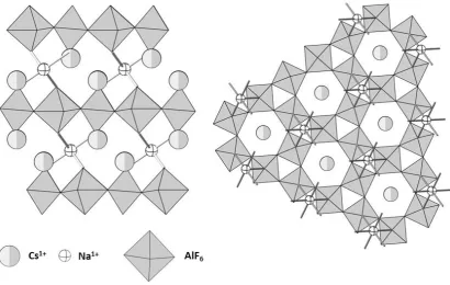
As can be seen above the majority of candidate quantum spin liquids have taken the form of kagome lattices with Cu2+ ions as the source of the S = ½ ion. One group of materials that may be a clear avenue of research is the family A2MCu3F12. This family of compounds is chemically very flexible and able to accommodate a range of A1+ and M4+ cations. The inspiration for the series is from the non-magnetic compound, Cs2NaAl3F12 which adopts a R ̅m unit cell and, importantly, consists of a perfect kagome lattice.52 This kagome lattice is based upon corner sharing AlF6 octahedra and the layers are linked by NaF6 octahedra. The Cs1+ ions occupy the spaces above or below the pores (Figure 1.18).

The first copper bearing members of the family were Cs2ZrCu3F12 and Cs2HfCu3F12 reported in 1995, both showing perfect kagome lattices at room temperature isotypic with Cs2NaAl3F12. At the time these were only briefly studied magnetically.53 Further magnetic study leads to the agreement of previous results but different origins are suggested. Rather than high temperature transitions being Néel temperatures, as originally suggested, it appears they are actually first order structural transitions (~ 210 K for Cs2ZrCu3F12 and ~ 175 K for Cs2HfCu3F12). Magnetic ordering is found at 23.5 and 24.5 K for M = Zr4+ and Hf4+, respectively. The magnetic ordering is found to be of antiferromagnetic character but due to spin canting presents itself as weakly ferromagnetic.54 Further structural investigations of Cs2ZrCu3F12 have found that there is a structural transition at ~ 225 K. This transition is characterised by a buckling of the kagome lattice – a F- ion in the planar section of the kagome lattice moves in order to increase the coordination number of Zr4+ to seven.55

Figure 1.18: Structure of Cs2NaAl3F12 looking along ab-plane (left) and down the c-axis (right).

18

there is a low temperature transition at ~ 185 K followed by long-range magnetic ordering at ~20 K. The structural change seen in magnetic susceptibility data appears to be different from that found for Cs2HfCu3F12 and Cs2ZrCu3F12 as it is much more subtle. The magnetic ordering is found to lead to no net magnetic moment parallel to the c-axis and a small moment perpendicular, indicating that again Néel ordering occurs but with some weak ferromagnetism, likely due to spin canting.56 Rb2SnCu3F12 is found to deviate from the crystal structures found for Cs2MCu3F12 (M = Zr4+, Hf4+, Sn4+); there is a doubling of the a and b parameters of the unit cell (in hexagonal axes) and the symmetry is reduced to R ̅.57 This is found to result from four different Cu2+ – Cu2+ bond distances, possibly related to the reduced size of Rb1+ compared to Cs1+ (1.61 Å vs. 1.74 Å for 8 coordinate, respectively49). There is also a disorder of the F- in the SnF6 octahedra. Magnetically, Rb2SnCu3F12 proves to be particularly interesting; it is found to be an example of a valence bond solid (VBS). This VBS state creates a pinwheel arrangement (Figure 1.19).39 Such an exotic state is promising as it suggests that these phases may be worth investigating as the substitutional flexibility may lead to the ability to tune and probe certain magnetic behaviours.

Another member of the family that shows a very different structural has also been synthesised; Cs2CeCu3F12. This sample has a highly corrugated kagome lattice due to the large Ce4+ becoming 7 coordinate (Figure 1.20); this leads to very different exchange interactions. The magnetic ordering is composed of one dimensional chains linking through CuF6 octahedra.58 Magnetically this leads to a complex system with the chains ordering antiferromagnetically but the Cu2+ between the chains is classed as “dangling”. It is found that these dangling spins have a complex ordering with half ordering ferromagnetically and half remaining paramagnetic.59

Figure 1.19: Kagome lattice in Rb2SnCu3F12 viewed down the c-axis, with ovals representing paired spins.

19

Figure 1.20: Cs2CeCu3F12 viewed along the ab-plane. Note the twisting of the kagome lattice compared to Figure

1.17 and the extra coordination of Ce4+.

The desired behaviour would be for a high-symmetry system like that found for Cs2SnCu3F12 to retain a perfect kagome lattice down to low temperatures, as opposed to the structural transition and magnetic ordering found. It can be seen that the identity of A and M plays a part in this by observing the structural transition temperatures of Cs2MCu3F12 (where M = Zr4+, Hf4+, Sn4+). It is also noted that there appear to be different behaviours even within this small series. It is suggested that by manipulating the ion size and identity it may be possible to avoid any structural phase transitions while also avoiding the imperfect kagome lattices found for Rb2SnCu3F12 and Cs2CeCu3F12.

1.3

Aims

20

The second aim of this work concerns the investigation of the effects of substitution on YMnO3. The substitution of Mn3+ by Fe3+ is of interested as they are isostructural but not isoelectronic. This could have interesting effects on the magnetic behaviour and also the ferroelectric behaviour and as yet has not been investigated in any detail. It is also of interest to observe the effect of a magnetic ion only being present on the Y3+ site. This can be achieved using trivalent lanthanides as substitutes for Y3+ and In3+ as a substitute for Mn3+.

1. N. A. Hill, J. Phys. Chem. B, 2000, 104, 6694-6709. 2. D. Khomskii, Physics, 2009, 2, 20.

3. M. Fiebig, J. Phys. D: Appl. Phys., 2005, 38, R123-R152. 4. A. Saunderson, Phys. Educ., 1968, 3, 272.

5. A. R. West, Basic Solid State Chemistry, Wiley, 1997.

6. M. J. Geselbracht, A. M. Cappellari, A. B. Ellis, M. A. Rzeznik and B. J. Johnson, J. Chem. Educ., 1994, 71, 696-703.

7. S. Sun, Adv. Mater., 2006, 18, 393-403.

8. D. Damjanovic, Rep. Prog. Phys., 1998, 61, 1267-1324. 9. R. E. Cohen, Nature, 1992, 358, 136-138.

10. G. Catalan and J. F. Scott, Adv. Mater., 2009, 21, 2463-2485.

11. B. B. Van Aken, T. T. M. Palstra, A. Filippetti and N. A. Spaldin, Nat. Mater., 2004, 3, 164-170.

12. E. Ascher, H. Rieder, H. Schmid and H. Stossel, J. Appl. Phys., 1966, 37, 1404-1405. 13. D. N. Astrov, R. V. Al'shin, R. V. Zorin and L. A. Drobyshev, Sov. Phys. JETP, 1969, 28,

1123-1125.

14. W. Brixel, J.-P. Rivera, A. Steiner and H. Schmid, Ferroelectrics, 1988, 79, 201-204. 15. J. Wang, J. B. Neaton, H. Zheng, V. Nagarajan, S. B. Ogale, B. Liu, D. Viehland, V.

Vaithyanathan, D. G. Schlom, U. V. Waghmare, N. A. Spaldin, K. M. Rabe, M. Wuttig and R. Ramesh, Science, 2003, 299, 1719-1722.

16. M. Grizalez, E. Martinez, J. Caicedo, J. Heiras and P. Prieto, Microelectron. J., 2008, 39, 1308-1310.

17. W. Eerenstein, N. D. Mathur and J. F. Scott, Nature, 2006, 442, 759-765. 18. H. Lueken, Angew. Chem. Int. Ed., 2008, 47, 8562-8564.

19. H. L. Yakel, W. C. Koehler, E. F. Bertaut and E. F. Forrat, Acta Crystallogr., 1963, 16. 20. J. E. Greedan, M. Bieringer, J. F. Britten, D. M. Giaquinta and H. C. Zurloye, J. Solid State

Chem., 1995, 116, 118-130.

21. T. Katsufuji, S. Mori, M. Masaki, Y. Moritomo, N. Yamamoto and H. Takagi, Phys. Rev. B, 2001, 64, 104419.

22. M. Fiebig, D. Frohlich, K. Kohn, S. Leute, T. Lottermoser, V. V. Pavlov and R. V. Pisarev,

Phys. Rev. Lett., 2000, 84, 5620-5623.

23. P. J. Brown and T. Chatterji, J. Phys. Condens. Matter, 2006, 18, 10085-10096.

24. T. Lonkai, D. G. Tomuta, U. Amann, J. Ihringer, R. W. A. Hendrikx, D. M. Tobbens and J. A. Mydosh, Phys. Rev. B, 2004, 69, 134108.

25. S. C. Abrahams, Acta Crystallogr., Sect. B: Struct. Sci., 2001, 57, 485-490.

26. D. Y. Cho, J. Y. Kim, B. G. Park, K. J. Rho, J. H. Park, H. J. Noh, B. J. Kim, S. J. Oh, H. M. Park, J. S. Ahn, H. Ishibashi, S. W. Cheong, J. H. Lee, P. Murugavel, T. W. Noh, A. Tanaka and T. Jo, Phys. Rev. Lett., 2007, 98, 217601.

21

28. A. S. Gibbs, K. S. Knight and P. Lightfoot, Phys. Rev. B, 2011, 83, 094111.

29. Z. J. Huang, Y. Cao, Y. Y. Sun, Y. Y. Xue and C. W. Chu, Phys. Rev. B, 1997, 56, 2623-2626.

30. T. Lottermoser, T. Lonkai, U. Amann, D. Hohlwein, J. Ihringer and M. Fiebig, Nature, 2004, 430, 541-544.

31. A. Harrison, J. Phys. Condens. Matter, 2004, 16, S553-S572. 32. A. P. Ramirez, Annu. Rev. Mater. Sci., 1994, 24, 453-480.

33. I. Mirebeau and S. Petit, Eur. Phys. J. Spec. Top., 2012, 213, 37-51.

34. Y. Okamoto, M. Nohara, H. Aruga-Katori and H. Takagi, Phys. Rev. Lett., 2007, 99, 137207.

35. K. R. Poeppelmeier and M. Azuma, Nat. Chem., 2011, 3, 758-759. 36. L. Balents, Nature, 2010, 464, 199-208.

37. P. A. Lee, Science, 2008, 321, 1306-1307.

38. P. W. Anderson, Mater. Res. Bull., 1973, 8, 153-160.

39. K. Matan, T. Ono, Y. Fukumoto, T. J. Sato, J. Yamaura, M. Yano, K. Morita and H. Tanaka, Nat. Phys., 2010, 6, 865-869.

40. L. Clark, J. C. Orain, F. Bert, M. A. De Vries, F. H. Aidoudi, R. E. Morris, P. Lightfoot, J. S. Lord, M. T. F. Telling, P. Bonville, J. P. Attfield, P. Mendels and A. Harrison, Phys. Rev. Lett., 2013, 110, 207208.

41. A. Olariu, P. Mendels, F. Bert, F. Duc, J. C. Trombe, M. A. de Vries and A. Harrison, Phys. Rev. Lett., 2008, 100, 087202.

42. R. S. W. Braithwaite, K. Mereiter, W. H. Paar and A. M. Clark, Mineral. Mag., 2004, 68, 527-539.

43. B. Fak, E. Kermarrec, L. Messio, B. Bernu, C. Lhuillier, F. Bert, P. Mendels, B. Koteswararao, F. Bouquet, J. Ollivier, A. D. Hillier, A. Amato, R. H. Colman and A. S. Wills, Phys. Rev. Lett., 2012, 109, 037208.

44. F. H. Aidoudi, D. W. Aldous, R. J. Goff, A. M. Z. Slawin, J. P. Attfield, R. E. Morris and P. Lightfoot, Nat. Chem., 2011, 3, 801-806.

45. M. P. Shores, E. A. Nytko, B. M. Bartlett and D. G. Nocera, J. Am. Chem. Soc., 2005, 127, 13462-13463.

46. P. Mendels, F. Bert, M. A. de Vries, A. Olariu, A. Harrison, F. Duc, J. C. Trombe, J. S. Lord, A. Amato and C. Baines, Phys. Rev. Lett., 2007, 98, 077204.

47. M. A. de Vries, J. R. Stewart, P. P. Deen, J. O. Piatek, G. J. Nilsen, H. M. Ronnow and A. Harrison, Phys. Rev. Lett., 2009, 103, 237201.

48. G. J. Nilsen, M. A. de Vries, J. R. Stewart, A. Harrison and H. M. Ronnow, J. Phys. Condens. Matter, 2013, 25, 106001.

49. R. D. Shannon, Acta Crystallogr., Sect. A: Found Crystallogr., 1976, 32, 751-767.

50. S. H. Lee, H. Kikuchi, Y. Qiu, B. Lake, Q. Huang, K. Habicht and K. Kiefer, Nat. Mater., 2007, 6, 853-857.

51. W. Krause, H. J. Bernhardt, R. S. W. Braithwaite, U. Kolitsch and R. Pritchard, Mineral. Mag., 2006, 70, 329-340.

52. G. Courbion, C. Jacoboni and R. Depape, Acta Crystallogr., Sect. B: Struct. Sci., 1976, 32, 3190-3193.

53. M. Muller and B. G. Muller, Z. Anorg. Allg. Chem., 1995, 621, 993-1000.

54. Y. Yamabe, T. Ono, T. Suto and H. Tanaka, J. Phys. Condens. Matter, 2007, 19, 145253. 55. S. A. Reisinger, C. C. Tang, S. P. Thompson, F. D. Morrison and P. Lightfoot, Chem.

Mater., 2011, 23, 4234-4240.

22

57. K. Morita, M. Yano, T. Ono, H. Tanaka, K. Fujii, H. Uekusa, Y. Narumi and K. Kindo, J. Phys. Soc. Jpn., 2008, 77, 043707.

58. T. Amemiya, M. Yano, K. Morita, I. Umegaki, T. Ono, H. Tanaka, K. Fujii and H. Uekusa,

Phys. Rev. B, 2009, 80, 100406.

59. T. Amemiya, I. Umegaki, H. Tanaka, T. Ono, A. Matsuo and K. Kindo, Phys. Rev. B, 2012,

23

24

The work presented in this thesis has made use of a variety of techniques. Prime among them is diffraction (Section 2.1) which has been used to probe, in detail, the structure of the materials synthesised. A number of other techniques have been used to acquire important further details of the materials synthesised; these include magnetometry (Section 2.2), A.C. impedance spectroscopy (Section 2.3) and Mössbauer spectroscopy (Section 2.4).

2.1

Diffraction

The majority of ionic solids present themselves in a crystalline ordered state. This means that they have long range order such that they can be represented as an infinite structure built up from the stacking of one, identical building block. These building blocks (or unit cells) can be divided into seven different crystal systems which describe their fundamental symmetry (Table 2.1).1

Table 2.1: The seven crystal systems.1

System Bravais

lattices

Axial

lengths Axial angles

Defining symmetry

Cubic P, I, F a = b = c α = β = γ = 90° 4 triads equally inclined at 109.47 °

Tetragonal P, I a = b ≠ c α = β = γ = 90° 1 rotation tetrad or inversion tetrad

Orthorhombic P, I, C, F a ≠ b ≠ c α = β = γ = 90° 3 diads equally inclined at 90 ° Trigonal P, R a = b = c α = β = γ ≠ 90° 1 rotation triad or inversion

triad

Hexagonal P a = b ≠ c α = β = 90°, γ = 120° 1 rotation hexad or inversion hexad

Monoclinic P, C a ≠ b ≠ c α = γ = 90° ≠ β 1 rotation diad or inversion diad

Triclinic P a ≠ b ≠ c α ≠ β ≠ γ None

The “Bravais lattices” referred to in Table 2.1 indicate the position of the nodes (or lattice points) of the unit cell, i.e. parts of space that can be considered as identical and therefore mark the ending of one cell and the beginning of the next. P stands for primitive and indicates that there are only nodes at the corners of the unit cell. I means body-centred and indicates that there are nodes at the corners of the unit cell and the body-centre. C is similar to body centred except, along with nodes at the corners, there is no node in the centre of the cell but the centre of two opposite faces. F indicates face-centred and means that there are nodes on the corner of the unit cell and the centre of each face (i.e. simultaneous A, B and C-centring).

25

regular spacings between them leads to these useful interference effects. The reason X-rays, in particular, cause this effect is due to the similarity in their wavelength and these spacings; ~ 10-10 m. The same effect is not found for other energies in the electromagnetic spectrum. A good, artificial construct which models the interaction of X-rays with a crystalline sample is to observe the arrangement of atoms as simplified flat planes (Figure 2.1).

Figure 2.1: A 2-dimensional lattice (black dots) showing some of the possible planes (dashed lines).

26

Figure 2.2: Two planes (dashed lines) and two waves diffracting (solid lines). The distance between the planes is indicated as “dhkl”.

Figure 2.2 shows a Bragg model with two planes and two waves, one reflecting off the first plane and one off the second. Diffraction makes use of constructive and destructive interference; if the waves are in phase when entering the material this means they must emerge in phase in order to give constructive interference. In terms of Figure 2.2 this means that wave 2 must travel the same distance as wave 1 plus an integer number of wavelengths; i.e. equation 2.1 must be satisfied.

2.1

(where xyz is the distance from x to y to z, n is an integer and λ is the wavelength)

From Figure 2.2 we can also find the key geometric relationships, equations 2.2 and 2.3.

2.2

2.3

If equations 2.1 and 2.3 are combined then we reach Bragg’s law,2 equation 2.4.

2.4

When Bragg’s law is satisfied then diffraction can occur.

27

∑

2.5

The terms in equation 2.5 are defined as follows:1

 fnis the atomic scattering factor of atom n which varies with each ion,

 hxn + kyn + lznare the fractional coordinates of atom n in the unit cell with repeat units x, y and z,

 2π is the phase difference between two waves,

 and i is present as the equation contains both real and imaginary parts which relate the phase difference to a wave relationship.

The atomic scattering factors vary between atoms and can vary even for atoms with the same number of electrons (Figure 2.3) – this is related to the size of the electron cloud which surrounds the atom in question.

Figure 2.3: Scattering factors for 3 different 10 electron atoms/ions (O2-,3 Ne and Si4+)4.

2.1.1 Diffraction in practice

28

Figure 2.4: Laue spots (black spots) and Debye-Scherrer cones (dashed lines) shown on the same image. In practice only one of these dominates. The centre of the circles is adjacent to the X-ray source.

The cones or spots can be picked up as areas of higher X-ray intensity. If we consider the powder case and a detector composed of a photographic film the length of the whole of 2θ then the Debye-Scherrer cones would cause parts of the film to become exposed, leaving lines (Figure 2.5).

29

Although photographic film can measure the presence of X-ray radiation modern techniques make use of electronic detectors such as charge coupled devices (CCDs). Modern systems can also make use of a number of X-ray sources including molybdenum, copper and silver; the basis of most laboratory systems being the acceleration of an electron across a potential difference into the metal of interest. This acceleration across a potential difference and into the metal leads to an ejection of a core electron which is swiftly followed by the dropping of an electron from a higher orbital into the vacant core orbital. As this second electron is now in a lower energy state it emits energy in the form of an X-ray. In general it is necessary to monochromate the X-ray source in order to achieve only one X-ray wavelength.

2.1.1.1 Structural model refinement

In most cases, diffraction data is used against a model structure that is then refined in order to best match the data. The derivation of this data is either by prior knowledge and comparison to analogous systems or by “solving” the data. The latter is commonplace for single crystal diffraction and is usually achieved by complex mathematical algorithms. Refinement of single crystal models can also be a complex process but generally involves the refinement of lattice parameters, atomic coordinates, thermal parameter, absorption and a number of further minor variables which can affect the resulting models pattern. In the case of powder diffraction we also have a key interest and modelling the peak shape. This is considerably important in Rietveld refinements as it can help to take overlapping peaks into account – something which occurs in powder diffraction due to the loss of dimensionality.

Divergence from a perfectly diffracted, infinite line to a peak with a width and possible asymmetry is due to a number of reasons and often needs to be taken into account before an accurate model can be established. From the sample there are two primary features that affect line width; crystallite size and microstrain. Both of these broaden the peak profile and it is also possible to retrieve information from them. Other key line width contributions are usually from the diffractometer itself. These can include axial divergence (asymmetry on low angle peaks), flat specimen effects (in Bragg-Brentano geometry this can cause asymmetry) and imperfections in the X-ray source image. A large number of these can be accounted for using pre-described mathematical functions. Key components of these functions are the Lorentzian and Gaussian line shapes as well as asymmetric components.5

30

Other frequently refined variables are the zero-point of the diffraction equipment and other geometric parameters which can change from set-up to set-up. Site occupancies in some samples can be less than one and this can be measured as it is directly related to the electron density. The background signal also needs to be taken into account in most cases – this is particularly important in powder diffraction refinements as it can be of similar magnitude to the Bragg peaks.

After all these variables have been refined it is often necessary to quantify to the proximity of the resultant model to the experimental data. This can be achieved by a number of statistical measures. Commonly in powder diffraction, and referred to in this thesis are Rp (equation 2.6) and wRp (equation 2.7).5

∑| |

∑ 2.6

{∑ ∑ }

2.7

Similar measures exist for single crystal diffraction. The use of these measures allows different models to be compared to each other and the effect of refining different variable to be noted. They are also critical in the validation of models especially from single crystal diffraction data.

2.1.2 Synchrotron X-ray diffraction

In order to increase the intensity of the available X-rays, for more in depth structural analysis for example, it is necessary to substitute the X-ray generation techniques commonly found in the laboratory and to increase their complexity significantly. This is generally achieved using a synchrotron. A synchrotron is a form of particle accelerator that consists of a circular vacuum tube containing packets of electrons travelling at approximately the speed of light. Large magnets provide energy to increase the speed of the electrons but due to relativistic effects they cannot increase and so the extra energy applied is released as electromagnetic energy. This takes the form of a broad spectrum but it is possible to tune the spectrum using special magnets which cause the electrons to move in waves. Further tuning can be performed ante-sample using specialist mirrors in order to provide monochromatic X-rays.

31 2.1.3 Neutron diffraction

The primary criterion for a wave to interact with a crystal lattice is a wavelength of a similar magnitude to the gaps between the lattice planes. Particles can also behave as waves due to quantum effects and this can be quantified by the de Broglie wavelength (equation 2.8).

2.8

(where m is the mass of the particle, v is the velocity and h is Planck’s constant)

It is found that – at the correct velocity – neutrons have an appropriate de Broglie wavelength and so can be used in diffraction experiments. Neutrons of the correct wavelength can be realised experimentally in two ways:

1. A fission reactor can be adapted to channel out some neutrons and the neutron flux subsequently monochromated. These neutrons are then directed towards the sample. In this case the scattering angle, θ, is the variable (so-called “angle-dispersive” mode). 2. A “spallation source” can be used. This involves firing protons at a heavy metal target

(usually tungsten) which causes the release of a wide spectrum of neutrons. In general, the protons are held in a synchrotron and ejected towards the target at known times. As the time of proton impact is known the time of neutron release is also known. The sample is then a known distance from the target and so the speed of the neutrons can be calculated and from that the wavelength. In this type of diffractometer the variable is wavelength, λ (so-called “energy-dispersive” mode).

Both systems are in widespread use and have their own advantages. In general, neutron diffraction has a number of advantages and disadvantages when compared to X-ray diffraction. Sample size is an issue however, the flux from either neutron source is substantially lower than from a synchrotron; this leads to large samples being required or long exposure times. Absorption effects can also be problematic and access to particular tables of data or isotopes may be required. One key advantage though is that the interaction of neutrons is not related to atomic number; thus neutrons can act as a stand-alone technique or as a complementary technique to X-ray diffraction.

2.1.3.1 Neutrons and the determination of magnetic structure

32

Figure 2.6: An arrangement of nuclei with antiferromagnetic ordering. The “nuclear” (or structural) unit cell is indicated by the solid line; the magnetic unit cell is indicated by the dashed line.

The symmetries of these magnetic unit cells can be different from the 230 space groups found when only crystal structures are considered, and have been compiled into their own class called Shubnikov groups. The Shubnikov groups take into account the extra inversions (“time-reversal symmetry”) that must be taken into account when dealing with spins and their symmetry relationships.

2.2

Magnetometry

The measurement of magnetic phenomena is a complex process and there are a number of ways by which it can be performed. The work in this thesis has made use of two different experimental methods; namely the SQUID (superconducting quantum interference device) magnetometer and the VSM (vibrating sample magnetometer).

Both these measurement systems are capable of determining the magnetic moment from the sample, which then requires further correction for the number of moles of either the sample or the magnetic ions within the sample, depending on further intentions for the data. Both systems are theoretically (and in most cases practically) capable of measuring both magnetisation as a function of temperature and as a function of applied magnetic field. In either case, the typical measurement consists of cooling the sample outside of a magnetic field before heating within one and measuring the magnetic moment. A second, usually directly commenced, measurement cools the sample in a field and heats the sample in the same field while also measuring the magnetic moment. Such measurements can also indicate the nature of the magnetic moment interactions.

2.2.1 SQUID magnetometer measurements

33

sensitive switch which allows magnetic measurements as low as 10-15 Tesla to be recorded. A measurement is performed in a magnetic field with the superconducting coil at its centre. The sample is drawn through this coil which, due to the magnetic moment of the sample, leads to a change in electric current. This change in current is proportional to the magnetic field and, as the superconducting coil is connected in a closed loop to the SQUID input coil, the current also changes by an equal amount in the SQUID. The SQUID itself acts as a linear current to voltage converter, which leads to an output voltage that is proportional to the magnetic field.6

2.2.2 VSM measurements

The operation of the VSM instrument is dependent upon the vibration of the sample through a conducting coil (the “pick-up coil”) in a magnetic field. The magnetised sample causes a change in voltage in the “pick-up” coil. It is this voltage that can be used to find the dipole moment of the sample (equation 2.9).

2.9

(where VRMS = root mean squared of the voltage induced in the coil, δ = vibration amplitude, ω = 2π × frequency, P = dipole moment and Q = geometry dependent constant).7

The VSM instrument is found to be inferior to the SQUID in terms of sensitivity.

2.3

Electrical measurements

Impedance spectroscopy is a technique used to measure the electrical properties of a material. It measures the impedance, Z, of a material; this is the material’s ability to restrict the flow of electrons, and it has two parts; a real component, Z’, which is related to the resistance of the material and an imaginary part, Z”, which is related to the capacitance of the material.

2.10

(where Z” also = 1/ωC; ω = 2π × frequency, C = capacitance)

If considered in this way a material can be simplified to a circuit with a capacitor and a resistor in parallel. A more thorough description of impedance is given by equation 2.11.

| | 2.11

(where V = voltage, I = current, t = time, θ = phase angle)8

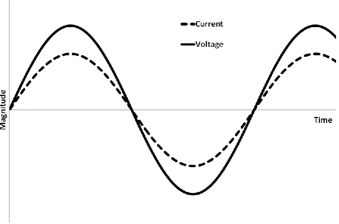
Phase angle, θ, differs for resistance and capacitance. Resistance follows ohms law (I= V/R) and so the current magnitude is directly related to the voltage; thus, θ = 0 (Figure 2.7). For a capacitor there is a key difference; as the voltage reaches a maximum the current stored reaches a maximum and so the current present in the circuit drops to zero. Then, when the voltage direction is inverted the current begins to reach a maximum as the stored charge is released. For a pure capacitor θ = 90 ° (Figure 2.8).

34

 M, electrical modulus

 Y, admittance (comprising Y’ = conductance, σ, and Y” = susceptance, which is related to 1/C)

 ε, dielectric permittivity (comprising ε’ = dielectric constant and ε” = dielectric loss)

In this work the main interest is the dielectric constant (or relative permittivity) and the dielectric loss. The former is the capacitive ability of the material and the latter is the dissipation of energy from the material as a side-product. Both these values can depend on the structure of the material and so lend themselves to locating phase transitions.

Figure 2.7: Current changing as a function of voltage through a resistor.

35

2.4

Mössbauer spectroscopy

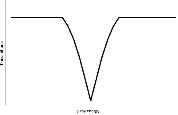
Mössbauer spectroscopy makes use of the resonant absorption of radiation by nuclei; emission of a photon by one nucleus and direct absorbance by another. Due to quantum mechanics, this can only occur if the energy if the photon is the same as one of the nuclear energy levels. Resonant absorption is found in the gas state for X-rays however higher energy γ-rays do not show this. This is due to the high energy of the γ-ray and conservation of momentum – when a γ-ray is released there is a large recoil on the emitting nucleus, the energy for which is taken from the emitted photon such that equation 2.12 holds.

2.12

(where E = energy (arbitrary units)

As the energy has been partially removed the emitted photon is no longer of the appropriate energy to be absorbed and so resonant absorption can no longer take place. In the case of a solid emitter and absorber however there are other considerations. The emission (and absorption) of a photon by a solid leads to a different form of recoil – the entire solid is unable to recoil and so internal lattice vibrations occur which act to dissipate the recoil energy. These lattice vibrations are quantum mechanical in nature, however, and so can only occur at specific energies, including zero. It is found that it is indeed possible to have a zero energy vibration and in effect a “recoil free event”. This is the Mössbauer effect.9

It is the Mössbauer effect that is manipulated in order to conduct highly sensitive spectroscopy. If suitable γ-rays are generated and emitted at a sample that can resonantly absorb these γ-rays then a few of the γ-rays will be absorbed. If there is a range of γ-rays around the required energy then a decrease in γ-ray transmittance is observed (Figure 2.9).