Fin whale density and distribution estimation using acoustic bearings derived from sparse 1
arrays 2
3
Authors: Danielle Harrisa, Jennifer Miksis-Oldsb,c,Julia Vernonb, Len Thomasa 4
5
Affiliations: 6
(a) Centre for Research into Ecological and Environmental Modelling, The Observatory, 7
Buchanan Gardens, University of St. Andrews, St. Andrews, Fife, KY16 9LZ, United 8
Kingdom. 9
10
(b) Applied Research Laboratory, The Pennsylvania State University 11
12
(c) School of Marine Science and Ocean Engineering, University of New Hampshire 13
14
Date resubmitted: 20 October 2017 15
16
Abstract 18
Passive acoustic monitoring of marine mammals is common, and it is now possible to 19
estimate absolute animal density from acoustic recordings. The most appropriate density 20
estimation method depends on how much detail about animals’ locations can be derived from 21
the recordings. Here, a method for estimating cetacean density using acoustic data is 22
presented, where only horizontal bearings to calling animals are estimable. This method also 23
requires knowledge of call signal-to-noise ratios (SNR), as well as auxiliary information 24
about call source levels, sound propagation, and call production rates. Results are presented 25
from simulations, and from a pilot study using recordings of fin whale (Balaenoptera 26
physalus) calls from Comprehensive Nuclear-Test-Ban Treaty Organization (CTBTO) 27
hydrophones at Wake Island in the Pacific Ocean. Simulations replicating different animal 28
distributions showed median biases in estimated call density of less than 2%. The estimated 29
average call density during the pilot study period (December 2007 - February 2008) was 0.02 30
calls.hr-1.km2 (coefficient of variation, CV: 15%). Using a tentative call production rate, 31
estimated average animal density was 0.54 animals/1000 km2 (CV: 52%). Calling animals 32
showed a varied spatial distribution around the northern hydrophone array, with most 33
detections occurring at bearings between 90 and 180 degrees. 34
I. INTRODUCTION 36
Using acoustic data to estimate animal density has been demonstrated for both terrestrial and 37
marine species (e.g., Buckland, 2006; Marquesetal., 2013, Stevensonet al., 2015). A suite 38
of density estimation methods exist that can be applied to different types of acoustic survey 39
data. The most appropriate density estimation method depends on how much detail about 40
animals’ locations can be derived from the recordings, which is often determined by the 41
number and configuration of deployed instruments. At best, three-dimensional locations of 42
calling animals can be estimated from acoustic data; conversely some recordings can yield 43
little to no information about animals’ locations. 44
Distance sampling (Buckland et al., 2001) and spatially explicit capture-recapture (SECR; 45
e.g., Borchers, 2012) are methods that estimate the probability of detecting animals (a key 46
parameter of any animal density estimation method) using spatial data collected during the 47
survey. Specifically, distance sampling can be used when the horizontal range between an 48
instrument and a calling animal can be estimated (e.g., Marques et al., 2011), which, for 49
marine animals, typically requires animal depth to be estimable (or assumed). SECR requires 50
that the same acoustic event is matched across multiple recorders, creating “capture histories” 51
of acoustic events. Indirect information about the location of calling animals can be inferred 52
from these capture histories by assessing which recorders (with known locations) detected the 53
acoustic events. Although SECR does not need measured ranges, SECR analyses can be 54
supplemented with data relating to animals’ locations such as direction, received sound level 55
and time of arrival (Borchers et al., 2015). Given their data requirements, both distance 56
sampling and SECR require arrays of recorders to estimate detection probability (though 57
horizontal ranges to calling animals can, in some particular scenarios, be estimated from 58
Conversely, when no spatial information can be estimated from recorded data (e.g., in most 60
scenarios where single instruments are deployed), detection probability can be estimated 61
using some form of auxiliary data. Marques et al. (2013) consider two types of auxiliary 62
information: (1) a sample of measured animal locations in relation to a recorder either from 63
animal-borne tags (e.g., Marqueset al., 2009) or combined visual and acoustic trials using 64
focal animals (e.g., Kyhnet al., 2012); (2) acoustic modeling using elements of the passive 65
sonar equation (Urick, 1983) including information about the target species’ call source level, 66
transmission loss, ambient noise levels, and the efficiency of the detection and classification 67
process. This latter information can be combined to estimate the probability of detection 68
using a simulation-based framework (e.g., Küseletal., 2011). Monte Carlo simulations have 69
been implemented for a range of cetacean species (Küselet al,2011; Harris, 2012; Helbleet 70
al., 2013; Frasieret al., 2016) but rely on accurate simulation inputs. One such input is the 71
distribution of simulated animals; however, there are often noa prioridata about what this 72
distribution should be. This is a key limitation of the Monte Carlo simulation approach. 73
Here, a new method is presented for estimating cetacean density using acoustic data, for cases 74
where horizontal bearings to calling animals are estimable. This approach is suitable for 75
scenarios where neither distance sampling nor SECR can be implemented, due to lack of 76
recorders (note that SECR survey design is an ongoing area of research but, to date, the 77
minimum number of recorders used for acoustic capture histories has been three, Kidneyet 78
al., 2016). The new method is related to the Monte Carlo simulation methodology as it uses 79
the passive sonar equation; measured call signal-to-noise ratios (SNR) are required, as well as 80
auxiliary information about call source levels, sound propagation, and call production rates. 81
However, the additional bearing data give some empirical information about animal 82
advantage of this method is that it produces a spatial map of estimated abundance (or 84
density), allowing inferences about spatial habitat preferences of acoustically active animals. 85
The paper is structured as follows. Section II presents a background to density estimation 86
using acoustic data, and a description of the new method. Details about the motivating case 87
study – fin whales recorded in the Pacific Ocean by Comprehensive Nuclear-Test-Ban Treaty 88
Organization (CTBTO) hydrophones – are given in Section III (including details of all the 89
required auxiliary analyses). Simulations are presented, which investigate method 90
performance under different known spatial animal distributions (Section IV). The method is 91
then applied to three months of recordings from Wake Island between December 2007 and 92
February 2008 (Section V). This analysis forms a pilot study prior to applying the method to 93
long-term CTBTO datasets from Wake Island and Diego Garcia in the Indian Ocean. Finally, 94
Section VI presents a discussion of the approach, including its limitations, benefits, and 95
potential implementations. 96
II. DENSITY ESTIMATION USING ACOUSTIC DATA 97
A general estimator of animal density using acoustic cues (e.g., animal calls) from static 98
instruments was presented by Marqueset al.(2009) (Eqn. 1): 99
(Eqn. 1) 100
where = call density, = number of detected signals, = false positive proportion, = 101
number of monitoring points, = maximum detection range, = average probability of 102
detection of an animal within radiusw of the sensor, = total monitoring time and =cue 103
production rate . This equation can be decomposed into three components: 104 r T P w K c n D a c ˆ ˆ ) ˆ 1 ( ˆ 2
Dˆ nc cˆ K
w Pˆa
ܦ=(ଵି̂)
ೌ ×
ଵ
గ௪మ×்ଵ̂ (Eqn. 2)
105
whereܰ=݊(1 −ܿƸ)⁄ܲ is the estimated abundance of cues,ܭߨݓଶis the area monitored, 106
so that dividing the abundance of cues by the area monitored gives a density of cues, and 107
1⁄ܶݎƸconverts the density of cues to the density of animals. 108
The average probability of detection, , can be estimated in several ways, as shown by the 109
variety of available density estimation methods (Marques et al. 2013). Each method has 110
various assumptions that must be met to produce an unbiased detection probability and hence 111
density. One key assumption in distance sampling is that the distribution of animals’ 112
distances from samplers (i.e., transect lines in a line transect survey, or monitoring points in a 113
point transect survey) is known. This is achieved by random placement of multiple samplers 114
within the study area so that, on average, animals are distributed uniformly in horizontal 115
space. For a survey using many fixed monitoring points with circular detection areas, this 116
assumed average distribution of animal distances is specifically a triangular distribution due 117
to the linear increase in area with increasing incremental horizontal distance from each 118
sample point (Buckland et al., 2001). However, when single acoustic stations are used, it 119
may not be reasonable to assume animal distances from that single station follow a triangular 120
distribution, and standard distance sampling should not be used to estimate (even if ranges 121
to animals can be estimated). Therefore, an alternative approach to estimating detection 122
probability is required. In the method developed here, cue abundance is estimated using a 123
Horvitz-Thompson-like estimator (after terminology used by Borchers & Burnham, 2004). 124
These estimators are based on seminal work by Horvitz & Thompson (1952), who showed 125
that when sampling at random from a population where each individual,i, has probabilityܲ 126
of being sampled, then an unbiased estimator of population size is given by the sum over 127
detected individuals of 1⁄ܲ. One can think of each detection “representing”, on average, 128
a Pˆ
1⁄ܲobjects in the population. In animal density estimation methods, individual detection 129
probabilities for every detection can be estimated (rather than estimating an average detection 130
probability as shown in Eqn. 1) and combined to give ܰ=∑ୀଵ 1⁄ܲ. However, the 131
detection probabilities, ܲ, are estimated, not known (hence “Horvitz-Thompson-like”). 132
Horvitz-Thompson-like estimators are not unbiased; the bias is typically small unless 133
estimated probabilities are highly uncertain or close to zero (Borcherset al., 2002). The key 134
advantage of this approach in the current case is that the individual detection probabilities can 135
be estimated without requiring any assumption about the distribution of animals with respect 136
to the samplers. 137
Other key assumptions that apply to this new method are that (1) all data measurements and 138
derived parameters are accurate and (2) detections are independent of one another. It is 139
highly improbable that recorded whale calls are produced independently of each other, given 140
that one animal may produce many calls. However, violation of the independence 141
assumption should not produce severe bias, though variance estimation can be affected 142
(Marques et al., 2013). Another assumption of any density estimation method is that 143
parameters used in the estimator are accurate for the time and place of the main survey. A 144
frequent limitation of auxiliary data used in density estimation analyses is that the additional 145
experiments (e.g., to estimate cue production rate) may have been conducted in a limited part 146
of the study area (or in a different location) and/or at a different time as the main survey, 147
which may lead to bias in the estimated parameters. Therefore, as many auxiliary analyses 148
should be undertaken using data from the main survey region and time period as possible. 149
A. Method overview 150
It is assumed that acoustic data have been recorded at known locations for a known time and 151
Estimation proceeds in the following stages, described in more detail in the next subsection. 153
1. Characterize the automatic detection process to estimate the probability of detecting a 154
call as a function of SNR (ܲ(ܴܵܰ)). The resulting fitted “detection characterization 155
curve” is used to estimate the detection probability for each detected signal. 156
2. Determine the monitored area: for each of a set of discrete bearings, use the assumed 157
call source level (SL) and the measured noise level (NL) distributions with a 158
transmission loss (TL) model to determine a set of ranges at which calls are almost 159
certain to be masked (i.e., the resulting SNR is so low that probability of detection is 160
very low) and exclude these areas from further analysis. 161
3. Estimate the distribution of possible ranges for each detection. Use the measured 162
received level (RL) and bearing of each detection, together with the assumed SL 163
distribution and TL model to estimate the probability density function (pdf) of ranges 164
for that detection. A probabilistic approach is required because (a) source level for 165
each detection is not assumed known, but is assumed to come from a probability 166
distribution; (b) even if source level were assumed known, the TL does not increase 167
monotonically with range and hence a detected signal with a given RL can correspond 168
to more than one range. 169
4. Estimate the range-specific distribution of number of signals corresponding to each 170
detection, i.e., scale each detection by its associated detection probability to account 171
for undetected signals. Using the Horvitz-Thompson-like estimator, each detection,i, 172
5. Estimate spatial density of signals by summing over the estimated number of signals 174
at each bearing and range to yield an empirical spatially-explicit abundance of signals. 175
Then smooth this using a Generalized Estimation Equation (GEE) spatial model. 176
6. Estimate animal density: use additional multipliers i.e., false positive proportion, time 177
spent monitoring (excluding periods of high ambient noise that cause masking) and 178
cue rate (Eqn. 1). Also potentially restrict inference to areas where detection 179
probability is higher and hence inference more reliable. 180
B. Further details 181
Stage 1: Characterize the automatic detector. Detector characterization is performed using a 182
sample of manually-detected calls. To ensure the sample is representative, a systematic 183
random subset of recordings (i.e., short sections equally spaced in time – see Section III for 184
an example) should be analysed manually. SNR is measured for a sample of manually-185
detected calls, as well as noting whether or not each call was detected by the automatic 186
detector. Logistic regression with automated detection/non-detection as the response and 187
SNR as the explanatory variable is used to model the probability of detecting a call as a 188
function of SNR. A Generalized Additive Model (GAM, Wood, 2006) is used to allow a 189
smooth, nonlinear relationship between probability of detection and SNR. The fitted detector 190
characterization curve is then used to predict probability of detection, ܲ(ܴܵܰ), for each 191
detection (over the entire monitoring period),ܲ=ܲ(ܴܵܰ). 192
If bearings cannot be estimated for all detections, one of two approaches can be taken: the 193
detector characterization curve can be estimated where a successful detection is defined as 194
either (1) any detected fin whale call (regardless of whether it had an associated bearing or 195
not), or (2) detected fin whale calls that had an associated bearing measurement. The choice 196
of detector characterization approach will affect the value used forncin the estimator (Eqn.
1). Under the first definition,ncwill be the number of detections (with or without measured
198
bearings); under the second definition,nc will be the number of detections with measured
199
bearings only. In both cases, an assumption is made that the measured bearings represent the 200
spatial distribution of all detected signals, including those for which bearings could not be 201
estimated. 202
Stage 2. Determine area monitored. This stage is analogous to identifying the maximum 203
detection range,w, in Eqn. 1, although a set of bearing-specific ranges are derived, allowing 204
TL to vary in different directions, and be non-monotonic with increasing range. Hence the 205
area monitored does not have to be circular or continuous. 206
SL is assumed to follow a normal distribution; so it is theoretically possible to detect calls 207
from implausibly large (or even infinite) ranges in Stage 3. Therefore, a pragmatic cut-off is 208
used that ensures detections from outside the area monitored will be very rare. The assumed 209
SL and NL distributions are evaluated at the 90th and 10th percentiles, respectively, to 210
represent a loud call in low noise. These values are used in the passive sonar equation along 211
with TL to calculate the SNR of the hypothetical call at various range and bearing steps 212
around the hydrophone (SL – TL – NL = SNR). The detection probability of the call at all 213
locations is evaluated from the detector characterization curve. Locations where the call has 214
a detection probability of equal to or less than 0.1 are considered to be acoustically masked. 215
The lowest TL associated with a masked location is used as a TL threshold to define 216
acoustically masked areas, which are then excluded from the remainder of the analysis. 217
Stage 3. Estimate distribution of possible ranges for each detection. Given a detection with 218
measured RL and bearing ߠ, the SL of the detection if the source was at range r can be 219
derived from the (simplified) passive sonar equation as 220
ܵܮ(ݎ,ߠ) =ܴܮ+ܶܮ(ݎ,ߠ) (Eqn. 3)
where ܶܮ(ݎ,ߠ) is range- and bearing-specific transmission loss. An SL distribution is 222
required, which is assumed to follow a normal distribution with mean ߤ and standard 223
deviationߪ. In this analysis, SL could be estimated from a subsample of localized calls at 224
short ranges. Then, the pdf of range is 225
݂(ݎ|ܴܮ,ߠ) =ఔ√ଶగఙଵ మ݁ି(ೄಽ(ೝమమ,ഇ)షഋ)మ (Eqn. 4) 226
whereߥis a normalizing constant to ensurefis a proper pdf: 227
ߥ=∫ √ଶగఙ మ݁ି
(ೄಽ(ೝ,ഇ)షഋ)మ
మమ
௪
ୀ ݀ݎ (Eqn. 5)
228
The need for an r in the denominator of Eqn. 4 is explained by viewing the analysis as 229
analogous to distance sampling with measurement error on the distances. In this case, the 230
geometry of a circular detection area means that random measurement error (in this case, 231
uncertainty in location) will result in underestimation of detections’ true locations (discussed 232
in Bucklandet al., 2015), leading to biased density estimates at closer ranges. 233
In practice, range is discretized into a fixed set of range intervals, with midpoints{ܴ}. TL is 234
calculated at these ranges, and it is assumed that the TL values apply to each corresponding 235
interval. Then, the probability a detection comes from intervalkis 236
Pr(݇|ܴܮ,ߠ) = (ோೖ|ோ,ఏ)
∑ೃೕ∈ೃ൫ோೕ|ோ,ఏ൯ (Eqn. 6)
237
Stage 4. Estimate range-specific distribution of number of signals corresponding to each 238
detection. SNR for each detected signal is calculated from the RL and NL measurements 239
associated with each signal (SNR = RL – NL). Detection probabilities of each detected 240
signal are estimated using the detector characterization curve and the range-specific 241
Horvitz-Thompson-like approach, the estimated number of signals in the population 243
“represented” by a signal detected with a given SNR is 1⁄ܲ(ܴܵܰ). Hence, the range-244
specific distribution of number of signals corresponding to a particular detection is given by 245
ܰ(݇|ܴܮ,ܰܮ,ߠ) =୰(ௌேோ)(|ோ,ఏ) (Eqn. 7) 246
Stage 5. Estimate spatial density of signals. At each bearing and range interval, the estimated 247
number of signals are summed. This yields a spatial abundance surface, but one that is not 248
necessarily smooth because of random variation in detections. Given a long monitoring 249
period, the true distribution of calls around the sensor likely is smooth, so precision can be 250
gained by smoothing the raw estimates using a GEE model (Hardin & Hilbe, 2012), which 251
accounts for spatial autocorrelation. The response variable is the estimated signal abundance, 252
assuming an overdispersed quasipoisson error distribution and using a log link function. 253
Explanatory variables are the location of the centre of the bearing and range interval in (x,y) 254
space (2-dimensional Cartesian coordinates). To account for the fact that intervals at larger 255
ranges represent a larger area, the area of each interval is included as an offset in the model. 256
To account for spatial autocorrelation, spatial blocks of 100 km x 100 km are created through 257
the study area and an independent working correlation structure implemented; model 258
residuals can therefore be correlated within blocks but are assumed to be independent 259
between spatial blocks. The spatial GEE is fitted using CReSS (Complex Region and Spatial 260
Smoother, Scott-Hayward et al, 2014) and SALSA (Spatially Adaptive Local Smoothing 261
Algorithm, Walkeret al., 2011) methods, allowing a flexible surface with spatially-varying 262
smoothness to be modeled. Model fit is assessed using concordance correlation and marginal 263
R squared values (in both cases, values close to 1 indicates good fit). A predicted density 264
surface is created by predicting abundance on a regular (x,y) grid, and dividing by the area of 265
Stage 6. Estimate animal density. The predicted density surface of signals is converted to a 267
predicted animal density surface by multiplying by(1 −ܿƸ)⁄ܶݎƸ, wherecis the false positive 268
proportion,Tis monitoring time, andrthe cue production rate. False positive proportion is 269
estimated from the manually-validated sample of data. Monitoring time should be known as 270
part of the survey protocol. Furthermore, the NL measurements of the detections can be 271
compared to ambient NL measured throughout the dataset to determine a NL threshold, 272
above which total acoustic masking is likely to occur. Time periods of data where ambient 273
NL exceeds the maximum NL associated with a detection are omitted from the monitoring 274
time,T. Cue production rate must come from auxiliary information and is often not known, 275
in which case density of calls can be estimated but not density of animals. 276
Average density can be computed by taking the average across the prediction surface. To 277
increase robustness, grid cells far from the sensor, where detection probability is low, may be 278
excluded from this averaging. A Horvitz-Thompson-like estimator is known to produce 279
positively biased estimates, particularly when some of theܲvalues are small (Borcherset al. 280
2002) as is the case for more distant calls. To mitigate this, a simulation study can be used to 281
determine at what range bias may be minimised and this can be used to truncate the range 282
over which average density is inferred. 283
C. Variance estimation 284
The delta method (Seber, 1982) is used to combine the coefficients of variation (CVs) for 285
each random variable used in the density estimator to estimate the overall CV for the 286
resulting density estimate. Note that the encounter rate also contributes to the overall 287
variance of a density estimate, and is denoted by in Eqn. 8. All other density 288
estimator inputs such as K, T and w are known constants and therefore do not have an 289
associated variance. 290
(Eqn. 8) 291
where: = overall mean probability of detection, defined as 292
݊/൫∑ୀଵ1⁄ܲ൯ (Eqn. 9)
293
In surveys with multiple samplers (i.e., monitored line or points), between-sampler variance 294
in encounter rate is usually estimated. With only one monitoring point as in this study, there 295
is no spatial variance in encounter rate and, instead, variance in encounters is linked only to 296
the detection process. Following guidance in Buckland et al., (2001), the encounters are 297
assumed to follow an overdispersed Poisson distribution. Therefore, encounter variance can 298
be estimated using the Poisson expression for variance (multiplied by a factor of 2 to 299
acknowledge assumed aggregation in the encounters) (Eqn. 10), which can then be used to 300
calculate the CV: 301
ݒܽݎ(݊) = 2݊ (Eqn. 10)
302
The false positive proportion and call production rate have weighted means (see Section III 303
for details) so variance is estimated using Cochran’s approximation (Cochran, 1997, 304
recommended by Gatz and Smith, 1995). Detection probability variance is estimated using 305
parametric bootstrapping of the SL and NL distributions, the coefficients of both the logistic 306
regression and GEE spatial models, then taking the empirical variance of the resulting 307
bootstrapped signal densities. As these signal densities are uncorrected for false positives, 308
the only parameter used in their estimation is ܲ, and so the signal density CV will be 309
equivalent to . 310
III. CASE STUDY - FIN WHALES IN THE PACIFIC OCEAN 311
The pilot study focused on fin whale calls recorded in the Pacific Ocean. Fin whales, the 312
second largest cetacean, occur globally and are currently listed as “Endangered” in the IUCN 313
2 2 2 22 ) ˆ ( ) ˆ ( ) ˆ ( ) ˆ
(D CV n CV c CV P CV r
CV c a
a Pˆ
)
ˆ
Red List (Reillyet al., 2013). Fin whales produce a low-frequency pulsed call, the “20-Hz” 314
call (Watkins et al., 1987), which has been widely utilized to investigate fin whales’ 315
distribution and density through passive acoustic monitoring (e.g., Širović et al., 2015). In 316
particular, a study of fin whales near Oahu, Hawaii, was an early example of using passive 317
acoustic data to estimate density (McDonald & Fox, 1999). Multipath arrivals and the 318
passive sonar equation were both used to estimate ranges to calling animals. However, 319
neither detection probability nor non-calling animals were explicitly accounted for, so the 320
resulting estimates were interpreted as a minimum number of animals (McDonald & Fox,
321
1999). 322
Data from the CTBTO IMS station at Wake Island (station identifier: H11) in the Equatorial 323
Pacific Ocean were used (1) as a basis for simulation studies to test the efficacy of the 324
method and (2) to demonstrate a pilot analysis using fin whale 20 Hz calls. Data from peak 325
seasonal detections from Dec. 1, 2007 to Feb. 29, 2008 were used, and details of data 326
processing and auxiliary analyses are given throughout the rest of this section. 327
A. Wake Island CTBTO IMS station 328
The Wake Island station is composed of two 3-element triangular arrays with 2.5 km spacing 329
between elements, with three hydrophones located to the north of the island (Fig. 1) and three 330
to the south. These cabled hydrophones are suspended in the deep sound channel. The three-331
month pilot study used data from the northern array (hydrophone depths were 731 m, 732 m, 332
and 729 m). The average water depth at the array was 1068 m (estimated from Amante & 333
Eakins, 2009). Sound levels were recorded continuously at a 250 Hz sampling rate and 24 bit 334
A/D resolution. The hydrophones were calibrated individually prior to initial deployment in 335
January 2002 and re-calibrated while at sea in 2011. All hydrophones had a flat (within 3 336
curves was applied to the data to obtain absolute values over the full frequency spectrum (5-338
115 Hz). Data less than 5 Hz and from 115-125 Hz were not used due to the steep frequency 339
response roll-off at these frequencies. 340
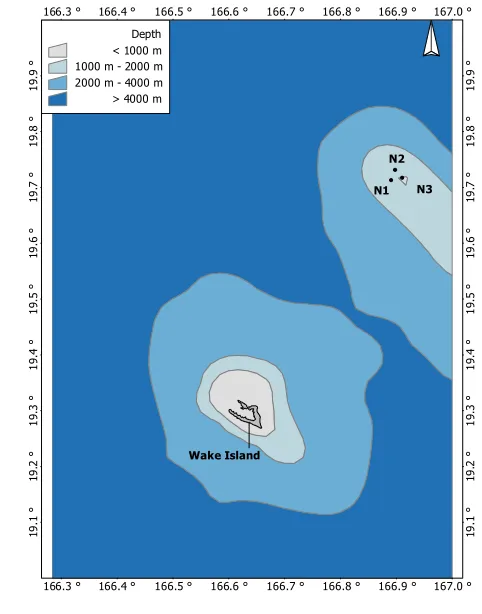
[image:16.595.93.334.138.445.2]341
Figure 1. Map showing the location of Wake Island (coordinates: 19.30, 166.63) and the 342
northern hydrophone array. Water depth contours (1000 m, 2000m and 4000 m) are also 343
depicted. 344
B. Transmission loss of a fin whale call 345
The transmission loss due to range-dependent propagation between a vocalizing whale using 346
a 20 Hz call and one of the northern hydrophone receivers (labelled N1) at 731 m depth was 347
modelled along 360 bearings at 1o resolution using the OASIS Peregrine parabolic equation 348
model out to 1000 km from N1 (Heaney & Campbell, 2016) (Fig. 2). The transmission loss 349
Depth < 1000 m 1000 m - 2000 m 2000 m - 4000 m > 4000 m
was modelled at 1 km range steps over the three-month study using seasonal sound speed 350
profiles obtained from The World Ocean Atlas
351
(https://www.nodc.noaa.gov/OC5/indprod.html). It was assumed that the source was at a 352
depth of 15 m, in keeping with results about fin whale calling behavior (Stimpert et al., 353
2015). The bathymetry was taken from the global bathymetry database ETOPO1 (Amante & 354
Eakins, 2009). Surface loss was negligible due to the low frequency of signals. Sea floor 355
parameters of soft sand sediment were used representing a global average of deep ocean 356
sediment. Details of the geoacoustics parameters in the specific Wake Island region are not 357
known but should not affect propagation in this environment due to direct path/sound channel 358
propagation. 359
360
[image:17.595.74.483.50.624.2]361
Figure 2. Transmission loss of a 20 Hz signal propagating from Wake Island N1 at a depth of 362
15 m. The model was run for every bearing between 0 and 359 degrees at 1 km range steps. 363
In this plot, 0 degrees indicates north. 364
C. Ambient noise levels 366
Mean spectral levels within the 10-30 Hz band were calculated for each minute of the three-367
month dataset, resulting in spectral levels with units of dB re 1 μPa2
/Hz. Ambient noise 368
levels were calculated in the targeted 10-30 Hz band to directly overlap with the frequency 369
range of the fin whale 20-Hz pulse. Mean spectral levels were calculated using a Hann 370
windowed 15,000 point Discrete Fourier Transform with no overlap to produce sequential 1-371
min power spectrum estimates. Note that these measurements included fin whale calls, 372
where present; it was important that the noise levels reflected all noise sources that each fin 373
whale call could be exposed to, which included calls by conspecifics. 374
D. Source level estimation 375
A sample of fin whale calls were localized using the northern array so that a source level 376
distribution could be estimated. Source level (SL) estimates of detected fin whale 377
vocalizations were computed using the passive sonar equation (Eqn. 11) that incorporated 378
environmental noise levels present at the time of the call within the received level (RL) of the 379
vocalization. 380
ܵܮ=ܴܮ+ܶܮ−ܦܫ+ܦܶ−ܲܩ (Eqn. 11)
381
As the low-frequency calls are omnidirectional, the directivity index (DI) was set to zero. 382
Processing gain (PG) and detection threshold (DT) are accounted for in the calibration of the 383
recording system. Received levels were calculated for individual vocalizations recorded at 384
N1 using a custom MATLAB (Mathworks, 2016) code. Spectrograms were calculated using 385
a 512-point FFT and 93.75% overlap. Calls were then manually detected, with a human 386
analyst selecting the upper and lower frequency and time bounds of an individual call. The 387
The TL of a signal of a given frequency is dependent on the range, bearing, and depth of the 389
vocalizing animal. The time difference of arrival (TDOA) between each hydrophone pair was 390
found by cross-correlation of received signals and was supplemented with manual inspection 391
due to dispersed waveforms. 2D hyperbolic localization was then used to find the range and 392
bearing of the vocalizing animal. Location information was then input into the site-specific, 393
seasonal transmission loss models to back calculate the SL of each identified vocalization. 394
The depths of the sources were unknown but assumed to be at a depth of 15 m following 395
results from Stimpertet al. (2015). For comparison, source levels of the same sample of calls 396
were also calculated using simple spherical spreading instead of the more complex Peregrine 397
transmission loss model. 398
E. Automated fin whale call detection 399
Fin whale calls were detected from the N1 hydrophone using the automatic detection feature 400
of Ishmael, an open-access bioacoustic analysis software package (Mellinger, 2002). The 401
spectrogram correlation method was utilized for the full three-month dataset, cross-402
correlating the spectrogram of the dataset with a synthetic call kernel. The kernel is a 403
template that indicates the time and frequency endpoints of the desired call. To prepare the 404
dataset for autodetection, time-waveform data were first passed through a 10-30 Hz bandpass 405
filter. Spectral data were then calculated using a 512-point FFT with a 93% overlap, and a 22-406
14 Hz one-second downsweep call kernel was applied. 407
Results from the automatic detector were compared with the manually detected calls from a 408
subset of data. The three-month dataset was divided into six-hour sections, and a systematic 409
random sample of these sections was taken. Every 11thsix-hour section was selected under 410
the sampling scheme, resulting in 32 six-hour sections. All calls within the 32 selected 411
automatic detector that compared the false positive proportion (the number of false positives 413
divided by the total number of automatic detections) with the proportion of missed calls (the 414
number of missed calls divided by the total number of manually detected calls, i.e., false 415
negative proportion) for a range of detection thresholds. The ROC curve indicated that the 416
optimal detection threshold had a 10% false positive proportion and a false negative 417
proportion of 59%. The mean false positive proportion was weighted by the number of 418
detections checked in each six-hour section. 419
F. Bearing measurements 420
Bearings were calculated using the TDOA of received signals. Using the known distances 421
between receivers and the seasonal sound speed, an estimated bearing was calculated for each 422
pair of hydrophones (Eqn. 12). 423
߮= arcsin(߬∗ܿ/݀) (Eqn. 12)
424 425
where ߬represents the TDOA of a signal between a hydrophone pair, d is the distance 426
between a hydrophone pair, andcis the speed of sound. 427
Left-right ambiguity of each bearing estimate could be resolved by comparing with the other 428
two estimates. The median bearing was then selected. An acceptable bearing is one where 429
the three bearings resulting from the three pair combinations all produced bearings within 10 430
degrees of each other. TDOA between each pair of hydrophones (N1 and N2, N2 and N3, N3 431
and N1) were found through three different methods, as described in order of application 432
below. If the cross-correlation method failed to produce an acceptable bearing, manual 433
estimation was performed. When manual estimation using the start point of each call failed 434
to produce an acceptable bearing, a band energy analysis was performed. The first step of all 435
methods was to pass the signals through a 10-30 Hz band pass filter. Bearings were rounded 436
(1) Cross-correlation 438
Once the data were filtered, a simple cross-correlation was performed in MATLAB to 439
determine time delays. Characteristics of the environment cause dispersion in the waveforms 440
traveling from distant ranges. As a result, a simple cross-correlation was not a viable option 441
for many of the distant calls. 442
(2) Manual Estimation 443
TDOA was found by manually selecting the start of each call from the time waveform. 444
Manual inspection eliminates the discrepancies that arise from the modal dispersion. Manual 445
selection also provided reliable results for calls with a low (< 6 dB) signal-to-noise ratio 446
(SNR), which is not always possible with automated methods. Manual detections were 447
feasible for a limited pilot study, but this method would not be appropriate for large datasets. 448
(3) Band Energy Analysis 449
Filtered data from N1 were analyzed in 3 Hz bands with 1 Hz overlap, starting at 10 Hz, 450
finding the peak in each band. The first band with a peak of at least 5 dB SNR was then 451
selected. The time index of the first peak in this frequency band for each sensor was then 452
noted and time delays were calculated from the identified time index. 453
G. Detector characterization 454
All calls were manually detected in the subsampled six-hour sections. The rms RL of each 455
call was measured, and the SNR of the call was calculated using a noise level measured from 456
the second of data preceding the call (in the same frequency bandwidth as the measured call 457
rms RL). Whether or not the call was detected by the automatic detector was also noted. The 458
3.3.1 (R Core Team, 2016). A GAM (Wood 2006) with a binary response and logit link 460
function was fitted to the data. 461
H. Call production rate 462
No call production rate data were available for fin whales occurring near Wake Island, but 463
call production rate data from the Southern California Bight in the North Pacific Ocean have 464
been published (Stimpert et al., 2015). The fin whale data from southern California were 465
collected in summer months, and so it is possible that this cue rate is biased for the fin whales 466
calling near Wake Island in the winter months. Cue rates from Stimpert et al. (2015) were 467
applied here as a proof of concept only, and resulting animal density estimates must be 468
treated cautiously. 469
IV. SIMULATION STUDIES 470
A. Simulation overview and input data 471
The primary aim of the simulation studies was to investigate whether the method returned 472
unbiased (1) detection probability estimates and (2) distribution maps under a range of 473
scenarios. To that end, call density only was estimated in the simulations (i.e., a false 474
positive proportion and call production rate were not considered). 475
Ambient noise and source level information, as well as the detector characterization curve, 476
were measured directly from the Wake Island dataset. The source level distribution (assumed 477
to be normally distributed) had a mean of 177.7 dB re 1 μPa2
/Hz @ 1m (standard deviation: 478
3.30, n = 79) using the Peregrine transmission loss model and 177.6 dB re 1 μPa2
/Hz @ 1m 479
(standard deviation: 3.03) using spherical spreading to predict propagation loss. Further, 480
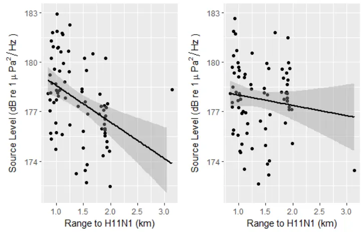
estimated source level decreased significantly as a function of range when using the 481
removal of three outlying data points using Cook’s distance measures). Estimated source 483
levels assuming spherical spreading also decreased slightly with range, though not 484
significantly (linear regression coefficient = -0.62, p-value = 0.27, n = 76) (Fig. 3). Given 485
that the means and standard deviations of the two source level distributions were almost 486
identical, the source level estimates using the more complex, bathymetry-dependent 487
Peregrine model were used for all simulations and analyses (though see Section VI for a 488
discussion of the regression results). The mean of the noise level distribution (also assumed 489
to be normally distributed) measured in association with manually detected calls was 92.5 dB 490
re 1 μPa2
/Hz (standard deviation: 2.74, n = 1484). The detector characterization curve was 491
estimated using 1484 manually detected calls, which were found in 20 out of 32 manually 492
checked six-hour sections (12 sections contained no calls). The mean SNR of automatically 493
detected calls was 13.98 (standard devation: 7.09, n = 612) and the mean SNR of calls missed 494
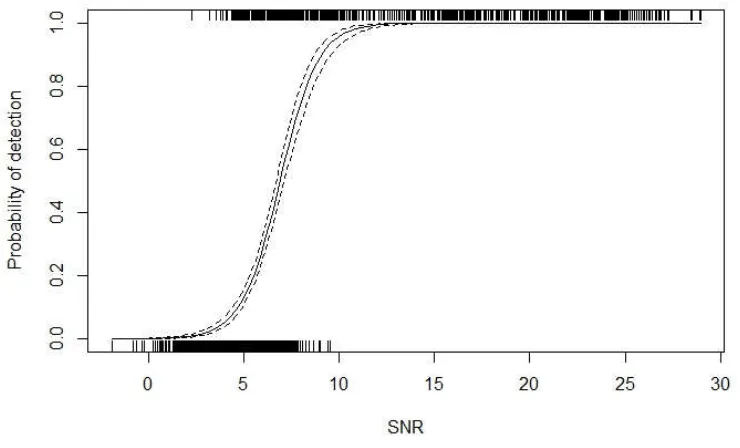
by the automatic detector was 4.45 (standard deviation: 1.59, n = 872). The fitted GAM 495
predicted that the majority of calls with an SNR greater than 10 dB were certain to be 496
498
Figure 3. Source levels estimated from 79 calls using transmission loss derived from (left) 499
the Peregrine model and (right) assuming spherical spreading. Both plots show a fitted linear 500
regression model (black line), with associated 95% confidence intervals shaded in gray. 501
503
Figure 4. Detector characterization curve (with 95% confidence interval) predicting detection 504
probability as a function of SNR for known fin whale calls (n = 1484). 505
506
Simulation TL data were based on TL data from Wake Island but were modified due to 507
extreme TL encountered in the real Wake Island data (see Section V). Wake Island TL data 508
were extracted at a depth of 15 m to reflect realistic fin whale calling behavior. TL ranged 509
between 71.70 dB and 286.46 dB. For the simulation studies, the minimum TL value (71.70 510
dB) was subtracted from all TL values resulting in simulated TL values that ranged between 511
0 and 214.76 dB. 512
Three call spatial distributions were tested via simulation, designed to reflect differing calling 513
animal distributions (Figure 5): calls were distributed (1) uniformly throughout the study 514
area, (2) limited to the north-east, and (3) limited to the south of the hydrophone. The 515
(1) Calls were simulated through the study area; call distribution were changed by drawing x-517
and y-coordinates from either a uniform or scaled beta distribution, depending on the desired 518
spatial call pattern (Fig. 5). 519
(2) Each simulated call was assigned an SNR based on the passive sonar equation; each call 520
was assigned a source level (SL) and noise level (NL) by drawing values from Normal 521
distributions with mean and standard deviations as measured from the Wake Island dataset, 522
which were then combined with the bearing- and range-specific TL value for that call, taken 523
from the modified TL data. 524
(3) Each call’s detection probability was evaluated from the detector characterization curve 525
and a Bernoulli trial was used to determine whether a given simulated call was detected or 526
not. 527
(4)The TL value above which no calls are detected was determined using the approach 528
530
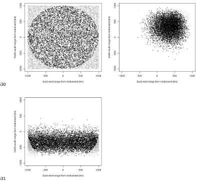
[image:27.595.79.475.78.443.2]531
Figure 5. Examples of distributions of simulated signals (clockwise from top left: uniform, 532
northeastern and southern distributions). The black dots denote signals within the 1000 km 533
maximum detection radius. Gray dots show signals outside the maximum detection range. 534
All simulations were run 500 times in R. The maximum detection range of the recording 535
system was specified as 1000 km in all cases. In both simulations and analyses, the 536
maximum detection range is set as an upper limit for a given instrument but may be reduced 537
when the monitored area is defined (Step 2, Section II.A). Call density or abundance (density 538
following the simulated detection process, the simulated RL, NL, and bearing values for each 540
simulated detected call were used as inputs for analysis instead of using measurements from 541
real recordings. In each of the three simulation scenarios, the initial abundance was altered 542
so that the number of detected calls was similar across all scenarios. The estimated call 543
density was compared to the known true value by calculating the median percentage bias 544
(with associated 2.5% and 97.5% percentiles). Additionally, because the true number of 545
simulated calls was known at increasing range steps from the array, the percentage bias as a 546
function of range from the array could also be assessed by comparing the true number of 547
simulated calls and the predicted number of calls within each range step. The maximum 548
range at which the percentage bias of call density was minimised was calculated for every 549
iteration (in some cases, the same minimal bias was calculated at multiple ranges, so the 550
largest range was selected). The distribution of these ranges could then be assessed after all 551
iterations were run to see whether there was an optimal prediction range, beyond which 552
percentage bias was likely to became larger, decreasing the robustness of the final predicted 553
density. This feature of the simulation algorithm may be useful for analysts to decide 554
whether to restrict the area of inference following an analysis to potentially reduce bias in the 555
reported density estimate. However, it is important to note that the simulation relies on an 556
assumed distribution of animal calls, which is likely to be different from the true, and 557
unknown, animal distribution, so a reduction in bias in analysis results is not guaranteed. 558
B. Simulation results 559
The simulations performed well – results from all scenarios had median percentage biases 560
less than 2% (Table 1). Percentage bias did not exceed 5% in any of the simulations. In 561
some scenarios, assessing the bias as a function of range showed that bias in call density 562
estimates could be substantially reduced when call density was inferred over a reduced range. 563
and 360 km, respectively, suggesting that these ranges were the optimal prediction ranges for 565
these scenarios. The NE distribution results were not improved by reducing the range of 566
prediction. Spatial model fit across scenarios varied, with uniform distribution models 567
displaying the poorest fit and the NE distribution producing spatial models with the best fit 568
(median marginal R squared values: 0.51, 0.79 and 0.92; median concordance correlation 569
values: 0.68, 0.88 and 0.96, for uniform, southern and NE distributions, respectively.). 570
However, all spatial models produced density maps that replicated the initial distributions 571
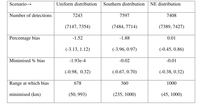
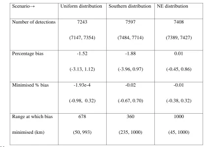
Table 1: Simulation results from three scenarios with different call distributions. Simulations 573
were run 500 times and all results report the median value, and the 2.5 and 97.5 percentiles in 574
parentheses. 575
Scenario→ Uniform distribution Southern distribution NE distribution
Number of detections 7243 (7147, 7354)
7597 (7484, 7714)
7408 (7389, 7427)
Percentage bias -1.52 (-3.13, 1.12)
-1.88 (-3.96, 0.97)
0.01 (-0.45, 0.86)
Minimised % bias -1.93e-4 (-0.98, 0.32)
-0.02 (-0.67, 0.70)
-0.01 (-0.38, 0.32)
Range at which bias minimised (km)
678 (50, 993)
360 (235, 1000)
577
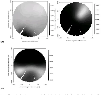
[image:31.595.74.484.75.461.2]578
Figure 6. Distribution maps of signal density (signals/km2) predicted by a Generalized 579
Estimating Equation . Initial simulated distributions were, clockwise from top left, uniform, 580
northeastern and southern distributions. The depicted maps are the median estimated surface 581
from 500 simulations. 582
583
V. PILOT STUDY 584
The pilot study analysis estimated fin whale density based on the detected calls (and 586
associated SNR and bearing measurements) from three months of data. A simulation was 587
also run to investigate the level of potential bias in the analysis results, and whether inferring 588
density over a smaller area may reduce any bias (as discussed in Sections II.B and IV.A). 589
Calls were uniformly distributed through the simulated study area and the steps of the 590
simulation set-up were the same as those described in Section IV.A, except for the TL data 591
used. 592
A key difference between the simulations described in Section IV.A and the pilot study 593
analysis and simulation was that unmodified TL data were used in the pilot study, reflecting 594
the true environmental conditions at Wake Island (Fig 7). 595
596
[image:32.595.105.430.372.548.2]597
Figure 7. Transmission loss of a 20 Hz signal propagating from Wake Island N1 at a depth of 598
without any unmeasurable infinite TL estimates (1231 km). The inset plot shows the same 600
data plotted up to 200 km; this inset shows the decrease in TL at ~ 50 km. 601
Inputs for the analysis were the following: number of detections, n, was 6552. The 602
automatic detector detected 6658 signals but the SNR of 106 signals fell below the lower 603
SNR limit of detected calls in the detector characterisation analysis (2.24 dB) and so were 604
removed to prevent model extrapolation when estimating detection probability using the 605
detector characterization curve. Of the remaining detections, 3086 (47%) had measurable 606
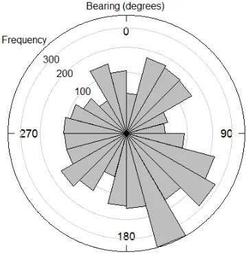
bearings, which ranged between 1.69 and 359.40 degrees (Fig. 8). While detections occurred 607
at all bearings around N1, the quadrant with the greatest number of detections occurred 608
between 90 and 180 degrees. 609
610
Figure 8. Histogram of measured bearings (in degrees) from the three-month pilot study 611
dataset (n = 3086). In this plot, 0 degrees indicates north. 612
The highest NL associated with a detection was 123.89 dB re 1 μPa2
/Hz. Of the 91 days of 613
continuous monitoring, 27 mins had an average NL of 124 dB re 1 μPa2
/Hz or above. 614
[image:33.595.151.330.316.513.2]detections taking place, so these periods were considered “off effort” and were excluded from 616
the time spent monitoring,T. 617
The false positive proportion,ܿƸ, was 0.097 (standard error: 0.05). The maximum detection 618
radius, where detection probability was assumed to be negligible, was set to 1000 km and a 619
total of 2183.55 hours were analysed (excluding 27 mins of recordings where ambient noise 620
was assumed to be too high to successfully run the automatic detector). 621
Call production rate was determined from Stimpertet al. (2015). Deployment duration and 622
number of calls recorded were reported for 18 digital acoustic recording tag (DTAGs, 623
Johnson & Tyack, 2003) records. Ten animals were tagged with a version of the DTAG (v3) 624
that enables calls from the tagged animal to be identified from other calls made by non-625
tagged conspecifics. It is crucial when estimating call production rate that only calls from the 626
focal animal are included in the analysis, so the other 8 animals tagged with v2 DTAGs were 627
omitted from the analysis. The v3 DTAGs were deployed between 1.60 and 6.30 hours. Six 628
tags did not record any calls, while the number of calls produced by the remaining four 629
tagged whales ranged between 23 and 942. The weighted mean call production rate was 630
45.08 calls.hr-1(standard error: 22.31). 631
632
B. Pilot study results 633
The pilot study simulation was run 500 times assuming a uniform distribution with an initial 634
starting abundance of 5e+6 calls, and a maximum detection range of 1000 km. The median 635
number of observations was 238, and the resulting median percentage bias in estimated 636
density was -56.37%, but decreased to -10.76% if density was only estimated up to a range 637
calls were predicted to originate was very restricted, compared to the detection area initially 639
considered (~12 million km2) and is fragmented (Fig. 9a). 640
The pilot study analysis estimated initial average call density over the three month period 641
from Dec 2007 – Feb 2008 to be 0.014 calls.hr-1.km2(CV: 0.15). Applying the call 642
production rate from the Southern Californian Bight resulted in an average fin whale density 643
of 0.32 animals.1000 km2.The CV for the density estimate was 0.52. The overall monitored 644
area for both the pilot study simulation and analysis (once spatial acoustic masking was taken 645
into consideration) was 973 km2(Fig. 9b). Based on the results of the simulation, the pilot 646
analysis results were re-analyzed with a range step restriction of 10 km. There was no way to 647
determine which of the detections without bearings would have been detected within 10 km, 648
so it was assumed that the relative abundances of the two detection types (which could be 649
calculated from the initial analysis across the whole survey region) was not altered by making 650
inference over a smaller area. Therefore, an additional multiplier,b, was used to scale the 651
estimated density based on detections with bearings (b =1.22). The resulting call density 652
estimate was 0.02 calls.hr-1.km2(CV: 0.15), which resulted in a density of 0.54 animals.1000 653
km2(95% confidence interval: 0.21 - 1.40 animals/1000 km2). The CV associated with the 654
656
Figure 9. Distribution maps of signal density (signals/km2) predicted by a Generalized 657
Estimating Equation based on the pilot study data inputs. Fig 9a (left) the median estimated 658
surface from 500 simulations. Fig 9b (right) the map from the analysis of fin whale calls 659
from the three-month pilot study (signals/km2). 660
661
VI. DISCUSSION 662
There are already several existing methods that can be used to estimate animal density from 663
acoustic data. However, the large variety of acoustic hardware and instrument configurations 664
continue to present new surveying challenges and require current density approaches to be 665
adapted. The CTBTO dataset presents such a case; there are 6 hydroacoustic stations similar 666
to Wake Island situated in the Pacific, Atlantic, and Indian Oceans (CTBTO, 2016), which 667
have provided a wealth of baleen whale recordings (e.g., Staffordet al., 2011, Samaranet al., 668
2013; Le Braset al., 2016). Each site is configured in a similar way to Wake Island, with 669
two triads of cabled hydrophones, one located to the north and one to the south of a land-670
based station that collects data round the clock. However, to date, it has not been possible to 671
method for CTBTO data: only two monitoring points would be formed by the two triads at 673
each site, which is too few for distance sampling (due to the animal distribution assumption 674
discussed in Section I). In addition, the array spacing within triads only enables call 675
localization using traditional time difference of arrival methods at close ranges, meaning that 676
detections from greater distances would have to be omitted from an analysis. Given that the 677
large detection ranges due to the deep sound channel moorings are an advantageous feature of 678
CTBTO hydrophones, distance sampling would not be an optimal analysis method in cases 679
where the majority of signals were originating from distant locations and could not be 680
localized (recently, however, Le Bras et al. (2015) presented an alternative location 681
methodology using bearing and amplitude information in a Bayesian framework to estimate 682
calling animals’ locations from CTBTO data, which may extend the localization capabilities 683
of these arrays). The array design at each site is also not configured well for an SECR 684
analysis. Although six hydrophones are available per site, acoustic masking is expected 685
between the northern and southern arrays, creating an acoustic barrier (Pulli & Upton, 2001). 686
Furthermore, the close spacing of the hydrophones in each triad would likely lead to many 687
detections being recorded by all three instruments. SECR depends on a variety of capture 688
histories to infer the location of calling animals; in this case, the array design may provide 689
limited information (i.e., scenarios where all instruments are ensonified on each occasion 690
yields little spatial information about the calling animals). 691
Therefore, data from the CTBTO arrays required a density estimation approach that used 692
auxiliary data. Although Monte Carlo simulations have been used to estimate call density of 693
blue whales in the Indian Ocean using CTBTO data (Harris, 2012), the method presented 694
here used the additional distributional information available in the measured bearings. The 695
more empirical data about animals’ locations that can be collected during the acoustic survey, 696
method was developed specifically for CTBTO data, there are other instrument systems that 698
record similar information. For example, DIFAR (directional frequency analysis and 699
recording) sonobuoys record bearings and have been used to detect blue whales at distances 700
over 100 nautical miles (e.g., Milleret al., 2015). 701
The simulations demonstrated that the method performed well under the three different 702
simulated animal distributions (though with less extreme propagation conditions as modelled 703
at Wake Island). In two of the three cases, bias was further reduced when density was 704
predicted over a smaller area than the detection radius originally set for the simulation. For 705
example, in the median surface plot of the uniform distribution scenario, an area on the 706
periphery of the detection radius has some negative bias (as shown by the darker region to the 707
south of the array in Fig. 6a) and the simulation results recommended that density only be 708
predicted out to 678 km. The same issue was also encountered during the pilot study. 709
Running a simulation specifically for the pilot study suggested that the initial estimates were 710
likely to be negatively biased and inference was restricted to a smaller area. In this case, 711
restricting the area nearly doubled the point estimate (from 0.32 to 0.54 animals.1000 km2). 712
In summary, the simulation code provides a tool for users to explore optimal detection ranges 713
for their given target species, survey location, and automated detection software. A natural 714
extension to the work would be to incorporate more complex animal distributions into the 715
simulation algorithm. 716
The pilot study analysis demonstrated how most of the required auxiliary data for this 717
approach can be generated using subsampled data from the main three-month survey. It is 718
crucial that all parameters in the density estimator have been estimated accurately for the time 719
and place of the main survey, otherwise resulting density estimates may be biased. Source 720
characterization curve were all estimated specifically for the Wake Island dataset. The source 722
level analysis suggested that, while the choice of transmission loss model made little 723
difference to the source level distribution parameters used in the simulations and analyses, the 724
negative relationship between estimated source level and range of the call from the 725
hydrophone when using the Peregrine transmission loss model warrants further investigation. 726
Parabolic equation models can have limitations at high incidence angles (i.e., small ranges in 727
this case) (Jensenet al., 2000), which could result in the discrepancies seen between the two 728
sets of source level results. Further, a fixed source depth of 15 m was assumed for all TL 729
data used in both the simulations and analyses; an extension to this work would be to see 730
whether changes in source depth (or using a distribution of source depths) significantly 731
affects the Peregrine TL (and therefore SL) results. The one parameter that could not be 732
estimated from the collected data was call production rate. In the absence of any other 733
available data, call production rates from the Southern Californian Bight collected during 734
summer months were applied to the estimated call densities. It is highly probable that the call 735
production rates of fin whales around Wake Island and southern California are different; cue 736
production rates do show spatiotemporal variation (e.g., Warrenet al., 2017). Therefore, the 737
fin whale densities estimated around Wake Island should be considered a “ballpark” estimate 738
at best. 739
The pilot study also demonstrated the flexibility of density estimation methods. In this case, 740
bearings could not be measured for all detections, but all detections (except those with SNR 741
values below the lower SNR limit of the detector characterization curve) could still be 742
incorporated into the analysis. It should be noted, however, that the estimated distribution 743
map was based on those detections with measurable bearings only. In order to interpret the 744
resulting distribution map as the predicted spatial distribution of calling fin whales, an 745
detections. In any method that makes assumptions, it is important to assess whether the 747
assumptions are reasonable, or whether they may have been violated. Therefore, 748
consideration should be given as to whether there are any oceanographic or bathymetric 749
features of the study area that may result in certain bearings being difficult, or impossible, to 750
measure (other than high TL values, which are accounted for by identifying areas of acoustic 751
masking at the start of the analysis). In these cases, the resulting map would not depict the 752
distribution of all calling animals. 753
The most striking result of the pilot analysis was the fact that the monitored area at Wake 754
Island for fin whale calls was much smaller than originally anticipated. Sirovicet al., (2007) 755
estimated detection ranges of fin whale calls in the Antarctic Ocean up to 56 km, though their 756
instruments were not moored in the deep sound channel. Previous work investigating 757
detection range of blue whale calls at CTBTO sites in the Indian Ocean (Samaran et al., 758
2010, Harris, 2012) predicted that blue whale calls could be detected hundreds of kilometres 759
away, facilitated by the deep sound channel. However, the pilot study results are supported 760
by previous work that predicted detectability of low frequency signals at Wake Island to be 761
lower than at Diego Garcia (Miksis-Oldset al., 2015). The results of all simulations and pilot 762
analysis also demonstrated that the monitored area may be an irregular shape, or even 763
fragmented, as seen in the pilot study. The fragmentation of the monitored area in the pilot 764
study is most likely caused by fluctuations in TL with range; the TL decreases at 765
approximately 50 km (Fig. 8, inset), which corresponds to the fragmented regions. 766
Monitored areas with unusual shapes should not lead to biased density estimates, as long as 767
the results are not extrapolated to areas outside the defined monitored area. 768
The pilot study has demonstrated the importance of quantifying the size and shape of the 769
monitored area (by estimating detection probabilities of the target species) during acoustic 770
oceanographic conditions change through the year. Geographic variability in detection 772
probability between sites, caused by local bathymetric and ocean conditions should also be 773
considered, even if the acoustic system is the same. Detection probability may also alter if 774
the behavior of the target species changes e.g., if animals increase call source levels in certain 775
behavioral contexts. Investigating such spatial and temporal variation in detection 776
probabilities at Wake Island and another CTBTO site, Diego Garcia in the Indian Ocean, will 777
comprise the next stage of this research. Another natural extension to this work would be to 778
analyse the southern site at Wake Island to investigate whether the same monitoring 779
conditions are present at a site ~ 200 km from the focal instrument in this initial study. 780
ACKNOWLEDGMENTS 781
DH and LT were funded by the Office of Naval Research (Award: N00014-14-1-0394). 782
JMO and JV were funded under Award: N00014-14-1-0397 also from the Office of Naval 783
Research. Kevin Heaney (OASIS, Inc.) generously contributed the TL modelling results for 784
which we extend sincere thanks. Thanks also to Lindesay Scott-Hayward for her help with 785
implementing CReSS and SALSA methods. The CTBTO data was accessed from the Air 786
Force Tactical Applications Center/US National Data Center. Thanks are extended to James 787
Neely (AFTAC), Richard Baumstark (AFTAC), Mark Prior (formerly CTBTO), and Andrew 788
Forbes (CTBTO) for their assistance in data transfer and transfer of knowledge of CTBTO 789
data. Thanks also to the CTBTO for making available the virtual Data Exploitation Center 790
(https://www.ctbto.org/specials/vdec/). Finally, please note that the views expressed in this 791
study are those of the authors and not necessarily represent the views of the CTBTO 792
REFERENCES 794
Amante, C. and B.W. Eakins, (2009) ETOPO1 1 Arc-Minute Global Relief Model: 795
Procedures, Data Sources and Analysis. NOAA Technical Memorandum NESDIS NGDC-24. 796
National Geophysical Data Center, NOAA. doi:10.7289/V5C8276M [02/01/2018]. 797
Borchers, D.L. 2012. A non-technical overview of spatially explicit capture recapture models. 798
Journal of Ornithology152 (Suppl 2), S435-444. 799
Borchers, D. L., Buckland, S. T. & Zucchini, W. (2002) Estimating Animal Abundance. 800
Springer,New York. 801
Borchers DL, Burnham KP. General formulation for distance sampling. In: Buckland ST, 802
Anderson DR, Burnham KP, Laake JL, Borchers DL, Thomas L, editors.Advanced Distance 803
Sampling. Oxford: Oxford University Press; 2004. pp. 6–30. 804
Borchers, D. L., B. C. Stevenson, D. Kidney, L. Thomas & T. A. Marques (2015) A Unifying 805
Model for Capture–Recapture and Distance Sampling Surveys of Wildlife 806
Populations,Journal of the American Statistical Association, 110:509, 195-204, DOI: 807
10.1080/01621459.2014.893884 808
Buckland, S. T. (2006) Point transect surveys for songbirds: robust methodologies.The Auk 809
123: 345-345 810
Buckland, S. T., Anderson, D. R., Burnham, K. P., Laake, J. L., Borchers, D. L. & Thomas, 811
L. (2001). Introduction to distance sampling - Estimating abundance of biological 812
populations. Oxford University Press, Oxford. 813
Buckland, ST, Rexstad, E, Marques, TA & Oedekoven, CS (2015) Distance Sampling: 814
Methods and Applications. Methods in Statistical Ecology, Springer. DOI:
10.1007/978-3-815
319-19219-2
816