Assessing the accuracy of land cover change with imperfect ground reference data
Foody, G. M.
Remote Sensing of Environment, 114, 2271-2285 (2010)
The manuscript of the above article revised after peer review and submitted to the journal for publication, follows. Please note that small changes may have been made after submission and the definitive version is that subsequently published as:
Assessing the accuracy of land cover change with imperfect ground reference data
Giles M. Foody School of Geography University of Nottingham
Nottingham NG7 2RD
UK
Abstract
The ground data used as a reference in the validation of land cover change products are often not an ideal gold standard but degraded by error. The effects of ground reference data error on the accuracy of land cover change detection and the accuracy of estimates of the extent of change was evaluated. Twelve data sets were simulated to allow the
exploration of the impacts of a spectrum of ground data imperfections on the estimation of the producer’s and user’s accuracy of change as well as of change extent. Simulated data were used since this ensured that the actual properties of the data were known and to exclude effects due to other sources of ground reference data error; although the impacts of simulated reference data on two real confusion matrices is also illustrated. The
imperfections evaluated ranged from the inclusion of small amounts of known error into the ground reference data through to the extreme situation in which ground data were absent. The results show that even small amounts of error in the ground reference data can introduce large error into studies of land cover change by remote sensing and
example, in the scenarios investigated, a 10% error in the reference data set introduced an under-estimation of the producer’s accuracy of 18.5% if the errors were independent but an over-estimation of the producer’s accuracy of 12.3% if the errors were correlated. The magnitude of the mis-estimation of the producer’s accuracy was also a function of the amount of change and greatest at low levels of change. The amount of land cover change estimated also varied greatly as a function of ground reference data error. Some possible methods to reduce or even remove the impacts of ground reference data error were illustrated. These ranged from simple algebraic means to estimate the actual values of accuracy and change extent if the imperfections were known through to a latent class analysis that allowed the assessment of classification accuracy and estimation of change extent without the use of ground reference data if the underlying model is defined appropriately.
1. Introduction
is, for example, one of the greatest causes of biodiversity loss and hence a central variable in studies of biodiversity conservation (Duro et al., 2007; Gillespie et al., 2008; Jones et al., 2009). Accurate and up-to-date information on land cover and land cover change is,
therefore, required for many applications.
Remote sensing is an attractive source of information on land cover and its dynamics at a range of spatial and temporal scales. However, numerous challenges are, or are perceived to be, encountered with the use of remote sensing for the derivation of information on land cover (Foody, 2002, 2008; Rindfuss et al., 2004; Strahler et al., 2006).
Considerable effort has been directed to the derivation of land cover information from remote sensing. At regional to global scales, for example, studies have developed from pioneering continental scale mapping programmes (e.g. Tucker et al. , 1985) to the situation today in which a variety of global maps are available (Herold et al., 2006; 2008). But many problems remain to be addressed. The large differences between maps of, apparently at least, the same phenomenon (Herold et al., 2006; See and Fritz, 2006; Potere et al., 2009) present user’s with uncertainty over which, if any, to adopt (Herold et al., 2008; Shao and Wu, 2008). Unfortunately this situation is not aided by the poor
The evaluation of map accuracy is now regarded as an important issue with accuracy assessment viewed by many as a fundamental component of mapping projects (Cihlar, 2000; Strahler et al., 2006). For those maps that have been evaluated, however, other problems often occur. Commonly, one problem is that remotely sensed land cover products are often viewed as failing to meet desired levels of accuracy (Townshend, 1992; Wilkinson, 1996; Gallego, 2004; Lu et al., 2008). This problem is particularly apparent in change detection based on post-classification comparison (Verbyla and Boles, 2000; Pontius and Lippitt, 2006). In such comparative assessments the amount of error in the classifications compared may obscure substantial change or could act to exaggerate change.
and is a hotspot of biodiversity, vary greatly from ~40 to ~80% (Jepson, 2005; Brannstrom and Filippi, 2008). Problems linked to the accuracy of the mapping by remote sensing have been highlighted as a major concern and source of uncertainty in many studies.
This paper aims to explore some of the key issues associated with one major, yet rarely studied, error in the remote sensing of land cover change and the possibilities to combat this error source in order to enhance the utility of remote sensing as a reliable source of land cover data. Building on Foody (2009), attention is directed to the impacts of imperfect ground reference data on the accuracy of land cover change estimation, perceived and real. A key focus is on the magnitude and direction of biases introduced into derived estimates of change detection accuracy and change extent arising through the use of imperfect ground reference data. The paper also aims to illustrate and explore some of the possibilities to reduce the negative impacts that arise through the use of imperfect ground reference data. The imperfections considered include the presence of ground reference data error, known and unknown, as well as situations when ground reference data are absent. It will be shown that in some circumstances the negative impacts of ground reference data error can be accommodated so that corrected or refined estimates may be made. Additionally it will be demonstrated that accuracy may still sometimes be assessed and estimates of the extent of change made when ground
some of the main scenarios encountered in remote sensing: the accuracy of change detection and the accuracy with which the amount or extent of change is estimated.
2. Estimation from a binary confusion matrix
Estimates of land cover change and of change detection accuracy are commonly made from a binary confusion matrix that illustrates the allocations to the change and no-change classes (Khorram, 1999; Congalton and Green, 2009). This approach has been widely used in a range of remote sensing studies (e.g. Woodcock et al., 2001; Chen et al., 2003; Stehman, 2005; Lunetta et al., 2006) and is the focus of this article. Critically, the distribution of entries in the confusion matrix together with the associated marginal values (row and column totals) may be used to derive numerous summary measures of the accuracy of the class allocations made and the amount of change that has occurred (Simon and Boring, 1990; Fielding and Bell, 1997; Khorram, 1999).
that provides a cross-tabulation of the remote sensing derived labels with those contained in a corresponding ground reference data set.
Since there is no standardised way of presenting the confusion matrix it will be assumed throughout this paper that the columns of the matrix represent the ground reference data and the rows the classification derived by remote sensing (Figure 1). The matrix provides a summary of the class labelling for the n cases used in a study, with each case lying within one of the matrix’s four elements. The latter elements are represented by the entries a to d in Figure 1. For simplicity, it will also be assumed that a representative sample of cases was acquired by simple random sampling, although many other designs may be used (e.g. Stehman, 2009).
Cases lying in elements a and d of the confusion matrix are those for which the labelling in the two data sets agree; in some literature these are referred to as true positives and true negatives (Staquet et al., 1981; Fielding and Bell, 1997). For the cases in elements b and c, however, the labelling in the two data sets differs; these are often referred to as false
positives and false negatives (Staquet et al., 1981; Fielding and Bell, 1997). The relative frequency of cases in the matrix elements may be used to describe the degree of
context of studies of land cover change, the confusion matrix provides information on the amount of land cover change and of change detection accuracy.
The accuracy of a binary classification is often described in terms of sensitivity and specificity (Rogan and Gladen, 1978; Staquet et al., 1981; Simon and Boring, 1990; Fielding and Bell, 1997). In the context of this article, the sensitivity of a classifier is the probability that the remote sensing method predicts change for a case of change, which can be expressed as the conditional probability P(R=1|∆=1)=S1 (Qu et al., 1996; Fielding and Bell, 1997). Thus, sensitivity is the proportion of cases correctly classified as having changed and may be derived from the confusion matrix from
e a c a
a
S
1 . (1)
The specificity of the classification is the probability of the remote sensing classifier predicting no-change for a case that has not changed, which can be expressed as the conditional probability P(R=0|∆=0)=S2. Specificity is, therefore, the proportion of cases correctly predicted to have not changed and may be derived from the confusion matrix using
f d d b
d
S
The sensitivity and specificity of the classification are, in the terminology used widely in the remote sensing literature, the producer’s accuracy (Liu et al., 2009) for the change and no-change classes respectively.
Reading the matrix horizontally allows the derivation of two additional measures, often referred to as the predicted positive value and the predicted negative value (Simon and Boring, 1990; Fielding and Bell, 1997). The former may be calculated from the confusion matrix by
g a b a
a
U
1 . (3)
The predicted negative value may be derived from the confusion matrix using
h d d c
d
U
2 . (4)
The positive and negative predicted values for the classification are, in the terminology used widely in the remote sensing literature, the user’s accuracy (Liu et al., 2009) for the change and no-change classes respectively.
n e d c b a c a
. (5)
Other measures may be derived but are not considered here. Often the values derived from equations 1-5 are multiplied by 100 to yield a value as a percentage.
Attention is focused in this paper on the sensitivity (producer’s accuracy for change) and prevalence (amount of change) estimates derived from the confusion matrix, although some comment will be made in relation to important issues connected with specificity and user’s accuracy. This focus is mainly because the producer’s accuracy and prevalence are typically of most interest in remote sensing studies but also because of relationships between the various measures. One key feature is that sensitivity (and specificity) is often viewed as being independent of prevalence (Rogan and Gladen, 1978; Staquet et al., 1981; Valenstein, 1990) but the positive and negative predicted values are a function of the quality of the classifier (indicted by its sensitivity and specificity) and the prevalence of change (Rogan and Gladen, 1978; Hui and Zhou, 1998; Simon and Boring, 1990; Enøe et al., 2001). The latter is evident in the expressions for U1 and U2 given in equations 6
and 7 respectively.
) 1 )( 1 ( 2 1 1
1
As a consequence of these relationships the positive predictive value (user’s accuracy of change) may be expected to increase if the prevalence of change increases (Staquet et al., 1981). In some disciplines, the prevalence dependency of U1 and U2 limits their value as general indices of classifier ability and accuracy as their magnitude has the undesirable property of fluctuating as a function of the variation in the variable under study. User’s accuracy may still, however, be a useful measure of accuracy in studies of the remote sensing of land cover change, indicating one aspect of classification quality for the specific area under study.
recognised as they may lead to substantial misinterpretation of change detection accuracy and extent. This paper focuses on some of the negative impacts arising from the use of imperfect ground reference data and the methods that may be used to reduce them. It builds on recent work on imperfect ground reference data (e.g. van Oort, 2005; Bruzzone and Persello, 2009; Carlotto, 2009; Foody, 2009; Pontius and Li, 2009; Pontius and Petrova, 2010), addressing some of issues highlighted as requiring attention such as the impacts of varying types of imperfection, including correlated errors, and even missing ground reference data.
Since the ground reference data set is a binary classification that, like that derived by remote sensing, may contain error its quality can also be characterised by a sensitivity and specificity. To distinguish between the ground reference and remotely sensed classifications, the sensitivity and specificity of the ground reference data will be represented by '
1
S and S2' respectively. Furthermore, since the imperfections of the ground reference data set impact on the perceived accuracy of the remote sensing classification, the ^ symbol will placed over estimates derived from a confusion matrix constructed with an imperfect ground reference data set (i.e., Sˆ1 is the estimate of the real sensitivity, S1, that is derived when imperfect rather than perfect reference data are used).
3. Ground data and their accuracy
may be deficient in relation to this attribute. Despite this situation, the ground reference data sets commonly used to evaluate the accuracy of land cover products derived from remote sensing are typically assumed to be correct or error-free (Foody, 2002; Carlotto, 2009).
The ground reference data used in a remote sensing project are unlikely to represent a gold standard as error may be contributed from a variety of sources. The latter include, for example, problems arising from mis-location of testing sites, presence of transitional classes, boundaries, typographical errors, restricted access to sites, uncertainties in class definition and temporal mismatches between image and field data acquisition (Powell et al., 2004; Comber et al., 2005; van Oort, 2005; See and Fritz, 2006; Thompson et al.,
2007; Bradley, 2009). The problems may be especially apparent in studies of change as there is a need for ground reference data relating to at least two time periods for a phenomenon that is typically relatively rare (Stehman, 2009). As a result, obtaining ground data may be difficult, limiting both the quality of the data in terms of labelling accuracy as well as the number of cases and their location for use in accuracy assessment. Problems in obtaining ground data have often been reported in the literature (e.g. Liu and Zhou, 2004; Lu et al., 2008) and some even seek to work without ground data (Baraldi et al., 2005; Bruzzone and Marconcini, 2009). Moreover, it is sometimes noted that
believed to be of higher quality than the remote sensing based classification that being evaluated (Stehman, 2009).
Although the accuracy of ground reference data is rarely known (Carlotto, 2009) a guide to the magnitude of error that may be present can be gleaned from the literature. For example, manual aerial photograph interpretation is often used as a source of ground reference data. Studies of inter-interpreter agreement in the analysis of imagery highlight, however, substantial disagreement in labelling, even when using fine spatial resolution imagery (e.g. very large scale aerial photography) and trained interpreters as a source of ground reference data. While the magnitude of the errors may be expected to vary from project to project (e.g. as a function of image properties, thematic resolution interpreter training and experience etc.) the magnitude of disagreement may be large. Powell et al. (2004), for example, report that interpreters disagreed on 30% of cases. Other studies have also shown considerable differences in class allocations. For example, in relation to data acquired by aerial photograph interpretation, Thompson et al. (2007) found
land cover to a target accuracy of ~85% (Weng, 2002; Yang and Lo, 2002; Rogan et al., 2003; Treitz and Rogan, 2004; Yang and Liu, 2005; Mundia and Aniya, 2005). Not only do many studies fail to achieve such accuracy (Wilkinson, 2005; Shao and Wu, 2008) but they are also implicitly stating that a ~15% error in the ground data set is tolerable. It should be recognised that the use of such sub-optimal reference data is also a reflection of the costs of acquiring high quality data. For example, it may be prohibitively costly to undertake a large programme of fieldwork or to acquire very fine spatial resolution imagery and so researchers are effectively compelled to use less than ideal data for reference purposes.
Critically, ground reference data error should not be ignored, no matter how convenient it may sometimes be to do so, as its effects may be substantial and may possibly be
correctable (Carlotto, 2009; Foody, 2009). There is, therefore, a need to understand the possible effects of ground reference data error and gain an appreciation of how to correct for them.
4. Data
Simulated data were mainly used in order to remove complexities and uncertainties linked to the impacts of sources of error other than ground reference data error. A series of data sets were generated to explore the impacts of imperfect ground reference data on the perceived accuracy of change detection and change extent as well as illustrate possible methods to correct for the effects of ground reference data error. Here, three different groups of data sets were formed to allow evaluation of the effect of and
correction for a variety of ground data imperfections on studies of land cover change. The data sets were designed to allow a spectrum of imperfections to be addressed. The
rather the problem of deriving information on the accuracy of land cover change estimates without the ability to consult ground data.
The simplest situation arises when the errors used in the data sets to form the confusion matrix are uncorrelated. This situation is often assumed. For example, errors have often been assumed to be independent in discussion of error propagation in post-classification change detection (Pontius and Lippitt, 2006). Additionally, ensemble approaches used to increase classification accuracy also commonly assume that the classifiers used have independent errors (Bruzzone et al., 2004). To explore issues connected with the use of an imperfect ground reference data set when the errors are independent from those in the remotely sensed data set, a series of binary confusion matrices were formed to represent scenarios arising from the cross-tabulation of classification outputs of known quality. The formation of a confusion matrix required the specification of the sensitivity and
literature are typically >65% (Wilkinson, 2005). In keeping with a common desire to classify classes to similar accuracy, it was assumed that the remote sensing technique had equal sensitivity and specificity although an example with unequal settings is also
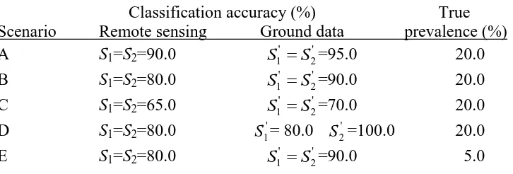
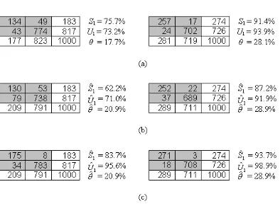
illustrated. Finally, a sample size of 1000 was used throughout and assumed to have been drawn by simple random sampling. The key details of the scenarios used are illustrated in Table 1. Since the properties of each scenario were known it was possible to construct the confusion matrix that would have been derived from the use of perfect ground reference data (S1' S2' 100%) as well as that arising from the use of the imperfect ground reference data (Figure 2).
Sometimes the errors in the ground and image classification are correlated. Correlated errors may arise in a number of ways and are sometimes noted in the remote sensing literature (Congalton, 1988; van Oort, 2005, 2007). For example, correlated errors may be expected if the classifiers have a similar basis and so tend to err on the same cases. Since correlated errors have a different impact to errors that are independent it is important to know the nature of the errors in the data sets used. Two classifications may be considered to be conditionally independent when the sensitivity (specificity) of one classification does not depend on the outcome of the other (Gardner et al., 2000; Georgiadis et al., 2003). The degree of dependence may be assessed using a measure such as the conditional correlation between the classification outcomes. For example, if the
conditional correlation between classification outcomes differs substantially from zero, the classifications may be considered conditionally dependent. The conditional
) 1 ( ) 1
( 12
2 1 1 1 1 1 2 1 1 1 * 1 1 S S S S S S S
(8)
for change and
) 1 ( ) 1
( 21 22 22
1 2 2 2 1 2 * 2 0 S S S S S S S
(9)
for no-change. where the super-scripts 1 and 2 indicate the two classifications under-comparison, S1* P(R11,R2 11)and S2* P(R1 0,R2 00). Further details on conditional dependence are given in the literature (e.g. Vacek, 1985; Qu et al., 1996; Branscum et al., 2005; Georgiadis et al., 2005). This paper focuses on situations in which the errors between the cross-classified data forming a confusion matrix are
independent (i.e. conditional independence exists) and when they are correlated (i.e. conditional dependence exists).
had S1' S2'= γ%, then 100-γ% of cases of change should be misclassified as no-change in both classifications and 100-γ% of no-change cases should be misclassified as
belonging to the change class in both classifications; see Valenstein (1990) for an example. Here, three scenarios, F, G and H, were simulated with 100-γ% set at 1.0, 2.0 and 10.0 % respectively (Figure 3).
In keeping with the desire to use a reference data set that is more accurate than the data set it is being used to evaluate, the errors introduced were small. Specifically, with map A a new matrix was simulated for the situation in which the ground reference data set was 95% accurate while for map B the accuracy was 98%; in each case it was assumed, for simplicity, that the sensitivity and specificity of the reference data classification were equal. The simulation was undertaken in the same fashion as described above for
independent and for correlated errors yielding new matrices based on imperfect reference data (Figure 4).
ensure that the errors contained were independent of each other and that represented by the output of the remote sensing classifier defined by scenario B. Indeed, the only major difference between the four classifications was the magnitude of accuracy.
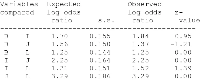
Finally, a further data set was generated to illustrate a method that may be used when the errors are both unknown and correlated. For this, the remotely sensed classification in scenario J was used as a base. A new data set was generated by copying the data in scenario J and then manually changing the class labels for 150 cases (50 cases that had actually changed and 100 cases that had not). In this way the new data set, forming scenario L, which was highly correlated to the data in scenario J but of a slightly lower accuracy was formed (Figure 5). The overall level of agreement between the
classifications in scenarios J and L was high, with agreement in labelling noted for 85% of the cases. Moreover, the magnitude of the conditional correlations between the data in scenarios J and L derived from equations 8 and 9 was large, substantially larger than zero and the value observed for other comparisons (Table 2).
5. Methods
derived estimates. Additionally, as the properties of the two classifications cross-tabulated to form each confusion matrix were known, it was possible to model the variation in the perceived accuracy of change detection as a function of the accuracy of the prevalence of change. That is, the known values of the sensitivity and specificity for each classification at a specified value of the true prevalence allow the derivation of the apparent sensitivity and specificity. Assuming the data sets to be conditionally
independent, this was achieved using equations 10 and 11 (Gart and Buck, 1966) for the perceived values of sensitivity
) 1 ( ) 1 ( )) 1 )( 1 ( ( ) 1 )( 1 ( ˆ ' 2 ' 1 ' 2 2 ' 2 1 ' 1 2 ' 2 1 S S S S S S S S S S (10)
and for specificity
) 1 ( ) ) 1 )( 1 (( ˆ ' 2 ' 1 ' 2 2 ' 2 1 ' 1 2 ' 2 2 S S S S S S S S S S
. (11)
against an imperfect ground reference data set of known accuracy. In recognition of the problems of obtaining information on ground reference data accuracy and to illustrate additional features, the second relates to the situation when there is no ground reference data but class allocation information from multiple classifications is available. This latter approach is based on latent class analysis.
5.1 Single classification and known ground data error
Although the quality of ground reference data will often be unknown it may sometimes be possible to estimate their accuracy (e.g. on the basis of prior experience or from acquisition of additional field based information etc.). If the accuracy of the ground reference data set is known and its errors are conditionally independent from those in the remote sensing based classification it is possible to derive the real change detection accuracy and extent of change from the observed confusion matrix. The correction for ground reference data error in this situation is derived algebraically with the real change detection accuracy and change extent derivable from simple equations (Gart and Buck, 1966; Rogan and Gladen, 1978; Staquet et al., 1981; Miller, 1998; Enøe et al., 2000). For the confusion matrix defined in Figure 1, the real producer’s accuracy of change may be derived from
e S
n
b gS S
) 1 ( 2'
' 2
1 . (12)
) 1 ( ) ( ' 2 ' 1 ' 2 1 1 S S g n S n e S
U (13)
Finally, a the real prevalence or amount of the extent of change may be derived from
) 1 ( ) 1 ( ' 2 ' 1 ' 2 S S n e S n
. (14)
Further details, including a discussion on the derivation of the relationships and formulae for standard errors of the estimates are given in the literature (e.g. Gart and Buck, 1966; Messam et al., 2008). The key concern for this article, however, is that, while ground reference data error is undesirable and can have substantial negative impacts on land cover change estimates researchers can do something about it.
5.2 Latent class analysis
The methods to correct estimates for ground reference data error defined by equations 12-14 may be used when the conditional independence assumption holds and the quality of the reference classification, expressed in terms of sensitivity and specificity, are known. However, both conditions may be hard to satisfy. Fortunately a range of alternative approaches exist to accommodate for the effects of ground reference data error (Espeland and Handelman, 1989; Qu et al., 1996; Hui and Zhou, 1998; Enøe et al., 2000). These approaches vary from methods that may be suited to situations when some properties of the ground reference data quality are known through to situations when there is no information on the quality of the ground reference data set and conditional independence cannot be assumed (Staquet et al., 1981; Hui and Zhou, 1998; Enøe et al., 2000). Indeed methods exist for extreme cases of imperfect ground reference data, such as when ground reference data are absent (Qu and Hadgu, 1998).
With no information on the quality of the ground reference data available more information or data on the problem than that contained in a single confusion matrix is required in order to allow reliable inferences to be drawn (Hui and Zhou, 1998; Enøe et al., 2000). This can be achieved in a variety of ways, notably by applying multiple
increasing the accuracy of classification through use of ensemble methods (Bruzzone et al., 2004).
The accuracy of a classification and estimates of prevalence can often be made in the absence of a perfect or gold standard reference data set through the use of a latent class model (Espeland and Handelman, 1989; Qu et al., 1996; Goethebeur et al., 2000; Enøe et al., 2001). Aside from one previous study on accuracy assessment (Patil and Taille,
2003), latent class models do not appear to have been used in remote sensing research and so some general background will be provided before presenting the models used.
In a standard latent class analysis it is assumed that the remote sensing based
A standard latent class model involving a single latent variable with two latent classes (change and no-change) and based upon the use of four independent classifiers, W, X, Y and Z, whose outputs are labels w, x, y, z = 0,1 is based on
WXYZ wxyzt t wxyzt
(15) with
Z
zt Y yt X xt W wt WXYZ
wxyzt
(16)
where WXYZwxyzt is the conditional probability that the pattern of class labels derived from the classifiers is (w,x,y,z) given that the case has a change status t (1 or 0) and tis the probability that a case has the change status t (Vermunt, 1997; Yang and Becker, 1997); note the classification outputs are variables in the analysis and so written in italics in the equations. Moreover, the conditional probabilities that represent the sensitivity and specificity of each classifier are parameters of the model (e.g. 11Wis the sensitivity of classifier W). The fit of a latent class model to the data is often evaluated with regard to a measure such as the likelihood ratio chi-squared statistic, L2; with a model normally viewed as fitting the data if the value of L2 is sufficiently small to be attributable to the effect of chance (Magidson and Vermunt, 2004).
prevalence (Espeland and Handelman, 1989; Hui and Zhou, 1998). For example, equation 16 is equivalent to the latent class log-linear model represented by equation 17,
Z zt Y yt X xt W wt t WXYZ
wxyzt
log (17)
where λ are the main effects of the true change status and the predictions made by the three classifiers (Hui and Zhou, 1998). As above, the sensitivity and specificity are directly related to model parameters and the prevalence of change is estimated as the proportion of the sample estimated to have changed in the latent variable (Espeland and Handelman, 1989).
The model components represented in equations 16 and 17 may also be adapted to allow for situations in which the assumption of conditional independence is untenable. For example, if classifiers Y and Z were not independent the model would use
YZ
yzt X xt W wt WXYZ
wxyzt
(18)
or, as the log-linear model,
YZ yzt Z zt Y yt X xt W wt t WXYZ
wxyzt
log (19)
of conditional independence is inappropriate its presence also means that the model’s parameters (e.g. Yytand Zzt in equation 19) no longer have a direct interpretation in terms of sensitivity and specificity for classifiers Y and Z (Yang and Becker, 1997; Hui and Zhou, 1998). Yang and Becker (1997) proposed parameterizing the log-linear model in marginal models in which a direct relation to sensitivity and specificity may still be made. Equation 19 is equivalent to a latent class marginal model that allows for dependence between classifiers Y and Z (Yang and Becker, 1997; Becker and Yang, 1998). In such a model the univariate marginal logits are directly related to sensitivity and specificity. Thus, for example, the sensitivity of classification Y may be estimated from
Y e S 1 1 1 1
(20)
where
YY
Y e 11 01 1
and its specificity from
Y Y e e S 0 0 1 2
(21)
where
Y Y Y e 10 00 0
(Yang and Becker, 1997; Hui and Zhou, 1998). Critically, it is evident
A test for conditional independence should be undertaken to ensure an appropriate model is used. A variety of approaches have been reported in the literature for assessing
conditional independence. Here, a modified version of the log-odds ratio check method (Garrett and Zeger, 2000), implemented using the CONDEP programme
(http://www.john-uebersax.com/stat/condep.html), was used. The log-odds ratio check
method is based on a comparison of the log-odds ratio for the observed (ψo) and expected (ψe) data, and the evaluation was based upon the comparison in terms of the z score
e e o z
(22)
and hence a value of z above the selected critical value indicates conditional dependence (e.g. for a two-sided test at the 0.05 level of significance the critical value is │1.96│).
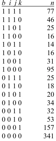
Here, latent class models were used to illustrate the potential to assess the accuracy of change detection and derive estimates of the extent of change when ground reference data were absent. This assessment was undertaken for the situation in which the classifications were conditionally independent and when they were conditionally dependent. First, using just the outputs from the remote sensing change detection classifiers defined in scenarios B, I, J and K, which were created in a manner that should ensure independence of errors, the approach represented by equations 15 and 16 was undertaken. Specifically, the model employed
K
kt J jt I it B bt BIJK
bijkt
and then was used to allow the producer’s accuracy (sensitivity) of each classifier and the prevalence of change to be estimated.
Finally, to illustrate the potential of the latent class modelling approach when correlated errors occur, a further analysis was undertaken. For this, the data in scenario K were replaced by those in scenario L, which was highly correlated with the data in scenario J. Then, the latent class model using
JL
jlt I it B bt BIJL
bijlt
(24)
was solved. The analyses based on equations 23 and 24 were undertaken with the LEM software (Vermunt 1997; software available at
http://www.uvt.nl/faculteiten/fsw/organisatie/departementen/mto/software2.html). Some
further analyses in which different dependence structures were specified were undertaken to explore the latent class modelling approach with these data.
however, the actual accuracy of the classification and amount of change was known as the data had been simulated with known properties. Finally, however, it is important to note that the focus in this paper is on the potential of the latent class analysis using simulated data of known properties for which it is relatively simple to define appropriate models. Real world applications may present a range of challenges and the validity of the approach and the ability to use it effectively requires further investigation. One critical feature is that, as a model based approach, it is important that the underlying assumptions of the model are satisfied.
6. Results and Discussion
Error in the ground reference data set impacted greatly on the perceived accuracy of change detection and of the amount of change that appeared to occur. The nature of the effect of ground reference data error varied greatly, especially in relation to whether the errors in the cross-tabulated data sets were independent or correlated. It may, however, be possible to correct for the negative effects of ground reference data error. The latter will be discussed after first evaluating the impacts arising from the use of an imperfect reference data set.
6.1 Independent errors.
For scenarios A-E it was apparent that ground reference data error introduced
was generally underestimated while the extent of change was over-estimated; of the scenarios investigated only scenario D did not follow this trend. Moreover, the magnitude of the bias introduced was large even when the ground reference data set was of very high accuracy. For example, in scenario A the ground reference data set was 95% accurate but caused a 13.9% underestimation of the producer’s accuracy (the perceived producer’s accuracy, Sˆ1, was estimated to be 76.1% but actually the real value, S1, was 90.0%). Not only was the magnitude of the bias large but it also had the effect of reducing the perceived accuracy below the popular 85% target, potentially leading to a highly accurate classification being wrongly rejected as not meeting the required
standard. Note also that the magnitude of the bias in producer’s accuracy increased with the amount of error in the ground reference data set, as evident from the results associated with scenarios A, B and C.
The prevalence or amount of change was also mis-estimated through the use of an imperfect ground reference data set. In all scenarios, the prevalence was over-estimated, rising from an estimate that was 3.0% larger than reality for scenario A to an 18.0% overestimation for scenario C. Indeed, in the latter scenario the amount of change was estimated to be nearly twice that which actually occurred.
39.3%, roughly half of the actual value of 80.0%. Additionally, the prevalence of change was substantially over-estimated, more so than with scenario B. Thus the accuracy of change detection by remote sensing and of change extent estimation was a function of the amount of change that has occurred; the estimates are prevalence-dependent. Moreover, the effect of variation in prevalence was modelled and revealed considerable impacts on the magnitude of the perceived accuracy (Gart and Buck, 1996). The relationship between the observed or perceived accuracy with prevalence is highlighted for the scenarios discussed in Figure 6. Note, for example, that the producer’s accuracy could vary greatly with prevalence. The producer’s accuracy was only independent of prevalence for scenario D.
The results from scenario D generally differed from the others. Scenario D was unusual in that the classification used as ground reference data had a perfect specificity. The consequence of this was that, for scenario D, the producer’s accuracy was estimated correctly. Moreover, the estimate of producer’s accuracy was not dependent on
Although not a major concern to this paper, it was also evident that substantial bias could be introduced by ground reference data error into the estimation of user’s accuracy. With user’s accuracy, the effect of ground reference data error varied in magnitude and the direction of the bias introduced also varied. For example, scenarios A and C show, respectively, under-estimation and over-estimation of user’s accuracy while the estimate for scenario B was correct (Figure 2).
6.2 Correlated errors
Ground reference data error sometimes caused substantial bias to the accuracy and extent estimates derived from a confusion matrix when there was correlation in the errors in the data sets cross-tabulated (Figure 3). The pattern in the results was, however, dissimilar to the general trend obtained with uncorrelated errors (Figure 2). Note, for example, that with correlated errors the producer’s accuracy was systematically mis-estimated but in the opposite direction to that generally observed with uncorrelated errors. Additionally, it was evident that the magnitude of the over-estimation of the producer’s accuracy was positively related to the degree of error, rising from scenario F through G to H (Figure 3).
The prevalence of change was also mis-estimated as a consequence of ground reference data error. For scenarios F to H, the prevalence of change was consistently
over-estimated. The bias introduced by ground reference data error into estimates of the user’s accuracy could be large, with U1 increasing from 50.0% to 75.0% in the scenarios
evaluated (Figure 3).
Errors that are correlated between the two data sets cross-tabulated to form a confusion matrix, therefore, impact differently to uncorrelated errors. Note, for example, the differences between scenarios B and H which were dissimilar in terms of the correlation between the data sets (Figures 2 and 3). Critically, each shows the impact of a 10% error in the ground reference data set. With both, the prevalence was over-estimated but in scenario B the producer’s accuracy for change was under-estimated by 18.5 % while it was over-estimated by 12.3 % in scenario H. Understanding the impacts of ground reference data error, therefore, requires information on the nature of the error and, in particular, the degree of correlation between the errors in the ground reference and image classification data sets used to form the confusion matrix.
6.1.3 Evaluation based on real matrices
amounts of error (Figure 4). Note also that the impacts affect other features. For example, the overall accuracy of a classification may be substantially mis-estimated (e.g. map A has an accuracy of 90.8% but appears to be 86.8% if errors are independent and 95.8% if errors are correlated). Moreover, the results from the analyses of the simulated data discussed above suggest that larger impacts would have been observed if the prevalence of change had been smaller than the relatively high values that had been recorded. The results highlight the need to address the effects of imperfect ground reference data in studies of land cover change by remote sensing.
6.1.4 Discussion
A key result highlighted above was that the use of imperfect ground reference data may sometimes result in a substantial mis-estimation of the amount of change, and so be a source of error contributing to the inaccuracy of change statistics reported in the literature. Ground data error also impacted greatly on the apparent accuracy of change detection. The impacts of ground reference data error varied as a function of the nature of the errors, notably in terms of their absolute and relative magnitude as well as direction of the bias introduced into estimates. Although there were some circumstances in which ground reference data error had no or only a small effect (e.g. on the estimation of producer’s accuracy in scenario D) they typically result in a false impression of classification accuracy and extent of change. Critically, however, the use of imperfect ground reference data can be a source of substantial error in studies of land cover change. Even when the ground reference data were very accurate the magnitude of the
should not be ignored. Indeed the problems of ground data quality should be considered in the design of a study, such as when planning the sample size of ground reference data sets (Rahme and Joseph, 1998; Messam et al., 2008) and in the interpretation of results. For example, the desire to sometimes focus attention disproportionately to hotspots of change (e.g. Broich et al., 2009) may result in problems linked to the prevalence
dependency of some accuracy measures. The results above highlighted, for instance, that the use of an imperfect ground reference data set may result in the apparent accuracy of change detection varying from location to location as a function of the prevalence of change. A classifier that was highly accurate at a location with considerable change may appear to be of low accuracy when applied to a location with little change. This problem could be interpreted as a failing of the classifier or perhaps the result of as some
transferability problem but may, at least in part, be a function of the use of imperfect ground reference data. The various problems of ground reference data quality noted reinforce the oft-stated call for the term ground truth to be avoided. Although truth is a concept and open to interpretation, the term ground truth may imply to some that the ground data set is error-free when this is unlikely and the imperfections of the ground reference data set, even if minor, can be a source of considerable error and mis-interpretation.
6.2 Correcting for ground reference data error
observed data in Figure 2 yields the real values, which are known as the data were simulated with known properties. That is, the estimate derived from the confusion matrix formed with regard to the imperfect ground reference data (e.g. Sˆ1) may be used to derive the real value (e.g. S1) through the use of the appropriate equation. These results reinforce calls made in other studies to use the confusion matrix for more than just a description of accuracy but as a means to refine estimates (van Oort 2005; Foody, 2009) and to provide the matrix as part of the accuracy statement. The results show that with known ground data quality, the real land cover change values may be derived by simple algebraic means.
dependency arose from the approach used to derive the data for scenario L from that in scenario J; the 150 cases for which the class label were changed were not selected randomly but from a data set ordered by perfect ground data which was in turn linked directly to the data for scenario B. Adjusting the model component in equation 24 to allow for a more complex dependence structure, including the dependence of B and L, and repeating the analysis resulted in a model that provided even closer fit to the data (L2= 37.71, df=2). Additionally, the estimates of accuracy and prevalence derived were close to reality (Table 10), although not necessarily closer than those derived from the earlier model, but the analysis was free from significant problems of conditional dependence (Table 11). It is worth stressing again, that the estimates of accuracy and change extent were derived without use of ground reference data.
Although the latent class modelling is more complex than the simple algebraic approach for the correction of the impacts of an imperfect reference it does appear to have
the need for ground reference data or from the potential to make erroneous estimation. The latent class modelling approach may sometimes offer an ability to constructively address ground reference data problems but its use does involve strong assumptions, especially if conditional dependence occurs, and so must be used with care. This paper has sought to show that ground reference data error may have substantial negative impacts on the remote sensing of land cover change but that sometimes it is possible to quantify these impacts and even implement corrective actions to reduce or remove them. Further work is needed to develop the latter, with the potential and limitations of latent class modelling, in particular, deserving greater attention in remote sensing.
7. Conclusions
The basis of change detection by remote sensing is very simple. In many applications the key information on change detection accuracy and amount or extent of change may be derived from a binary change detection matrix that is no more than a cross-tabulation of the labels contained the ground reference data set against those in derived from the remote sensing change detection analysis. There are, however, many sources of error in studies of land cover change and this paper focused on just one issue, the problems arising from the use of an imperfect ground reference data set.
understood and, aside from a few studies such as Hagen (2003), very little action taken to address negative effects. However, the results have shown that even small errors in the ground reference data set may introduce large bias into the derived estimates and so it is extremely unsafe to assume an error-free or gold standard reference data set. Fortunately, there are sometimes ways to address the problems caused by ground reference data error. Some methods that may be used were illustrated in this paper for a range of situations. It was stressed that the nature of the errors, especially in relation to the underlying
assumptions of the techniques, has important implications that should not be ignored as deviation from the assumed condition can have a major negative effect on the analysis. While this article has focused on the potential of techniques such as latent class
modelling in remote sensing further investigation is required. The latter should explore the limitations of latent class modelling and its suitability for use in typical remote sensing contexts. None-the-less, the potential to reduce or even remove the bias caused by ground reference data error has been indicated and this may help the effective use of remote sensing as a source of information on land cover change. The techniques
discussed are, of course, also applicable beyond studies of change, notably to other binary classification problems.
In summary, the four main conclusions of this paper are:
1. Ground reference data error can be a source of considerable error and
reference data set vary with the nature of the errors it contains (e.g. if correlated or not with the errors in the remotely sensed data).
2. The magnitude of the producer’s accuracy (sensitivity) can, contrary to
widespread belief in some communities, vary as a function of the prevalence of change if an imperfect ground reference data set is used. The use of an imperfect reference data set also impacts on the user’s and overall classification accuracy. 3. It is sometimes possible to reduce or even remove the effects of ground data error.
Moreover, it is sometimes possible to derive accurate estimates of change detection accuracy and extent without ground data. Note that the approach founded on latent class analysis is based on a model and the satisfaction of the model assumptions is critical in its use.
4. Ground data error and its impacts should be considered in the interpretation of studies of land cover change.
Acknowledgments
References
Achard, F., Eva, H. D., Stibig, H-J., Mayaux, P., Gallego, J., Richards, T. and Malingreau, J-P. (2002) Determination of deforestation rates of the world’s humid tropical forests, Science, 297, 999-1002.
Albert, P. S., and Dodd, L. E. (2004) A cautionary note on the robustness of latent class models for estimating diagnostic error without a gold standard, Biometrics, 60, 427-435.
Albert, P. S., McShane, L. M. and Shih, J. H. (2001) Latent class modeling approaches for assessing diagnostic error without a gold standard: With applications to p53
immunohistochemical assays in bladder tumors, Biometrics, 57, 610-619.
Alonzo, T. A., Pepe, M. S. and Moskowitz, C. S. (2002) Sample size calculations for comparative studies of medical tests for detecting presence of disease, Statistics in Medicine, 21, 835-852.
Becker, M. P. and Yang, I. (1998) Latent class marginal models for cross-classifications of counts, Sociological Methodology, 28, 293-325.
Bradley, B. A. (2009) Accuracy assessment of mixed land cover using a GIS-designed sampling scheme, International Journal of Remote Sensing, 30, 3515-3529.
Branscum, A. J., Gardner, I. A. and Johnson, W. O. (2005) Estimation of diagnostic-test sensitivity and specificity through Bayesian modeling, Preventive Veterinary Medicine, 68, 145-163.
Brannstrom, C. and Filippi, A. M. (2008) Remote classification of Cerrado (Savanna) and agricultural land covers in northeastern Brazil, Geocarto International, 23, 109-134.
Brannstrom, C., Jepson, W., Filippi, A. M., Redo, D., Xu, Z. and Ganesh, S. (2008) Land change in the Brazilian Savanna (Cerrado), 1986-2002: comparative analysis and
implications for land-use policy, Land Use Policy, 25, 579-595.
Bruzzone, L. and Marconcini, M. (2009) Toward the automatic updating of land-cover maps by a domain-adaptation SVM classifier and a circular validation strategy, IEEE Transactions on Geoscience and Remote Sensing, 47, 1108-1122.
Bruzzone, L. and Persello, C. (2009) A novel context-sensitive semisupervised SVM classifier robust to mislabeled training samples, IEEE Transactions on Geoscience and Remote Sensing, 47, 2142-2154.
Bruzzone, L., Cossu, R. and Vernazza, G. (2004) Detection of land-cover transitions by combining multidate classifiers, Pattern Recognition Letters, 25, 1491-1500.
Buck, A. A. and Gart, J. J. (1966) Comparison of a screening test and a reference test in epidemiologic studies. I Indices of agreement and their relationship to prevalence, American Journal of Epidemiology, 83, 586-592.
Carlotto, M. J. (2009) Effect of errors in ground truth on classification accuracy, International Journal of Remote Sensing, 30, in press.
Chen, J., Gong, P., He, C., Pu, R. and Shi, P. (2003) Land-use/land-cover change detection using improved change-vector analysis, Photogrammetric Engineering and Remote Sensing, 69, 369-379.
Comber, A., Fisher, P. and Wadsworth, R. (2005) What is land cover? Environment and Planning B, 32, 199-209.
Congalton, R. G. (1988) Using spatial auto-correlation analysis to explore the errors in maps generated from remotely sensed data, Photogrammetric Engineering and Remote Sensing, 54, 587-592.
Congalton, R. G. (1991) A review of assessing the accuracy of classifications of remotely sensed data, Remote Sensing of Environment, 37, 35-46.
Congalton, R. G. and Green, K. (2009) Assessing the Accuracy of Remotely Sensed Data: Principles and Practices, second edition, Boca Raton, Lewis Publishers
Dale, V. H. (1997) The relationship between land-use change and climate change, Ecological Applications, 7, 753-769.
Duro, D., Coops, N. C., Wulder, M. A. and Han, T. (2007) Development of a large area biodiversity monitoring system driven by remote sensing, Progress in Physical
Geography, 31, 235-260.
Enøe, C., Georgiadis, M. P. and Johnson, W. O. (2000) Estimation of sensitivity and specificity of diagnostic tests and disease prevalence when the true disease state is unknown, Preventive Veterinary Medicine, 45, 61-81.
Enøe, C., Anderson, S., Sørensen, V. and Willeberg, P. (2001) Estimation of sensitivity, specicity and predictive values of two serologic tests for the detection of antibodies against Actinobacillus pleuropneumoniae serotype 2 in the absence of a reference test (gold standard), Preventive Veterinary Medicine, 51, 227-243.
Engels, E. A., Sinclair, M. D., Biggar, R. J., Whitby, D., Ebbesen, P., Goedert, J. J. and Gastwirth, J. L. (2000) Latent class analysis of human herpesvirus 8 assay performance and infection prevalence in sub-saharan Africa and Malta, International Journal of Cancer, 88, 1003-1008.
Espeland, M. A. and Handelman, S. L. (1989) Using latent class models to characterize and assess relative error in discrete measurements, Biometrics, 45, 587-599.
Fielding, A. H. and Bell, J. F. (1997) A review of methods for the assessment of
prediction errors in conservation presence/absence models, Environmental Conservation, 24, 38-49.
Foody, G. M. (2002) Status of land cover classification accuracy assessment, Remote Sensing of Environment, 80, 185-201.
Foody, G. M. (2008) Harshness in image classification accuracy assessment, International Journal of Remote Sensing, 29, 3137-3158.
Foody, G. M. (2009) The impact of imperfect ground reference data on the accuracy of land cover change estimation, International Journal of Remote Sensing, 30, 3275-3281.
Foulds, S. A. and Macklin, M. G. (2006) Holocene land-use change and its impact on river basin dynamics in Great Britain and Ireland, Progress in Physical Geography, 30, 589-604.
Gardner, I. A., Stryhn, H., Lind, P. and Collins, M. T. (2000) Conditional dependence between tests affects the diagnosis and surveillance of animal diseases, Preventive Veterinary Medicine, 45, 107-122.
Garrett, E. S. and Zeger, S. L. (2000) Latent class model diagnosis, Biometrics, 56, 1055-1067.
Gart, J. J. and Buck, A. A. (1966) Comparison of a screening test and a reference test in epidemiologic studies: II a probabilistic model for the comparison of diagnostic tests, American Journal of Epidemiology, 83, 593-602.
Georgiadis, M., Johnson, W. O., Garner, I. A. and Singh, R. (2003) Correlation-adjusted estimation of sensitivity and specificity of two diagnostic tests, Applied Statistics, 52, 63-78.
Gillespie, T. W., Foody, G. M., Rocchini, D., Giorgi, A. P. and Saatchi, S. (2008) Measuring and modelling biodiversity from space, Progress in Physical Geography, 32, 203-221.
Hagen, A (2003) Fuzzy set approach to assessing similarity of categorical maps, International Journal of Geographical Information Science, 17, 235-249.
Hawkins, D. M., Garrett, J. A. and Stephenson, B. (2001) Some issues in resolution of diagnostic tests using an imperfect gold standard, Statistics in Medicine, 20, 1987-2001.
Herold, M., Woodcock, C. E., di Gregorio, A., Mayaux, P., Belward, A. S., Latham, J. and Schmullius, C. (2006) A joint initiative for harmonization of land cover data sets, IEEE Transactions on Geoscience and Remote Sensing, 44, 1719-1727.
Herold, M., Mayaux, P., Woodcock, C. E., Baccini, A. and Schmullius, C. (2008) Some challenges in global land cover mapping: An assessment of agreement and accuracy in existing 1 km datasets, Remote Sensing of Environment, 112, 2538-2556.
Hui, S. L. and Zhou, X. H. (1998) Evaluation of diagnostic tests without gold standards, Statistical Methods in Medical Research, 7, 354-370.
Jepson, W. (2005) A disappearing biome? Reconsidering land-cover change in the Brazilian savanna, The Geographical Journal, 171, 99-111.
Jones, D. A., Hansen, A. J., Bly, K., Doherty, K., Verschuyl, J. P., Paugh, J. I., Carle, R. and Story, S. J. (2009) Monitoring land use and cover around parks: a conceptual
approach, Remote Sensing of Environment, 113, 1346-1356.
Justice, C., Belward, A., Morisette, J., Lewis, P., Privette, J. and Baret, F. (2000) Developments in the ‘validation’ of satellite sensor products for the study of the land surface, International Journal of Remote Sensing, 21, 3383-3390.
Kennedy, R. E., Townsend, P. A., Gross, J. E., Cohen, W. B., Bolstad, P., Wang, Y. Q. and Adams, P. (2009) Remote sensing change detection tools for natural resource managers: understanding concepts and tradeoffs in the design of landscape monitoring projects, Remote Sensing of Environment, 113, 1382-1396.
Kintisch, E. (2007) Improved monitoring of rainforests helps pierce haze of deforestation, Science, 316, 536-537.
Khorram, S. (Ed), (1999) Accuracy Assessment of Remote Sensing-Derived Change Detection, (Bethesda, MD: American Society for Photogrammetry and Remote Sensing).
Liu, H. and Zhou, Q. (2004) Accuracy analysis of remote sensing change detection by rule-based rationality evaluation with post-classification comparison, International Journal of Remote Sensing, 25, 1037-1050.
Lunetta, R. S., Knight, J. F., Ediriwickrema, J., Lyon, J. G. and Worthy, L. D. (2006) Land-cover change detection using multi-temporal MODIS NDVI data, Remote Sensing of Environment, 105, 142-154.
Lu, D., Batistella, M., Moran, E. and de Miranda, E. E. (2008) A comparative study of Landsat TM and SPOT HRG images for vegetation classification in the Brazilian Amazon, Photogrammetric Engineering and Remote Sensing, 74, 311-321.
Magidson, J. and Vermunt, J. K. (2004) Latent class models, In Kaplan, D (editor) The SAGE Handbook of Quantitative Methodology for the Social Sciences, Sage, Thousand
Oaks, 175-198.
Mann, S. and Rothley, K. D. (2006) Sensitivity of Landsat/IKONOS accuracy
comparison to errors in photointerpreted reference data and variations in test point sets, International Journal of Remote Sensing, 27, 5027-5036.
McAlpine, C. A. Syktus, J., Ryan J. G., Deo, R. C., McKeon, G. M., McGowan, H. A., and Phinn, S. R. (2009) A continent under stress: interactions, feedbacks and risks associated with impact of modified land cover on Australia's climate, Global Change Biology, 15, 2206-2223.
Messam, L. L. McV., Branscum, A. J., Collins, M. T. and Gardner, I. A. (2008) Frequentist and Bayesian approaches to prevalence estimation using examples from Johne’s disease, Animal Health Research Reviews, 9, 1-23.
Miller, W. C. (1998) Can we do better than discrepant analysis for new diagnostic test evaluation, Clinical Infectious Diseases, 27, 1186-1193.
Mundia, C. N. and Aniya, M. (2005) Analysis of land use/cover changes and urban expansion of Nairobi city using remote sensing and GIS, International Journal of Remote Sensing, 26, 2831-2849.
Patil, G. P. and Taillie, C. (2003) Modeling and interpreting the accuracy assessment error matrix for a doubly classified map, Environmental and Ecological Statistics, 10, 357-373.
Pontius, R. G. and Lippitt, C. D. (2006) Can error explain map differences over time? Cartography and Geographic Information Science, 33, 159-171.
Pontius, R. G. and Petrova, S. H. (2010) Assessing a predictive model of land change using uncertain data, Environmental Modelling and Software, 25, 299-309.
Potere, D., Schneider, A., Angel, S. and Civco, D. A. (2009) Mapping urban areas on a global scale: which of the eight maps now available is more accurate? International Journal of Remote Sensing, 30, (in press).
Powell, R. L., Matzke, N., de Souza, C., Clark, M., Numata, I., Hess, L. L. and Roberts, D. A. (2004) Sources of error in accuracy assessment of thematic land-cover maps in the Brazilian Amazon, Remote Sensing of Environment, 90, 221-234.
Qu, Y. and Hadgu, A. (1998) A model for evaluating sensitivity and specificity for correlated diagnostic tests in efficacy studies with an imperfect reference test, Journal of the American Statistical Association, 93, 920-928.
Rahme, E. and Joseph, L. (1998) Estimating the prevalence of a rare disease: adjusted maximum likelihood, The Statistician, 47, 149-158.
Rindfuss, R. R., Walsh, S. J., Turner Ii, B. L., Fox, J. and Mishra, V. (2004) Developing a science of land change: challenges and methodological issues, Proceedings of the
National Academy of Sciences USA, 101, 13976-13981.
Rindskopf, D. (2002) The use of latent class analysis in medical diagnosis, Proceedings of the Annual Meeting of the American Statistical Association, American Statistical
Association, Alexandria VA, 2912-2916.
Rindskopf, D. and Rindskopf, W. (1986) The value of latent class analysis in medical diagnosis, Statistics in Medicine, 5, 21-27.
Rogan, J., Miller, J., Stow, D., Franklin, J., Levien, L. and Fischer, C. (2003) Land-cover change monitoring with classification trees using Landsat TM and ancillary data,
Photogrammetric Engineering and Remote Sensing, 69, 793-804.
See, L .M.and Fritz, S. (2006) A method to compare and improve land cover datasets: Application to the GLC-2000 and MODIS land cover products, IEEE Transactions on Geoscience and Remote Sensing, 44, 1740-1746.
Shao, G. and Wu, J. (2008) On the accuracy of landscape pattern analysis using remote sensing data, Landscape Ecology, 23, 505-511.
Simon, D. and Boring, J. R. (1990) Sensitivity, Specicity and predictive value, In H. K. Walker, W. D. Hall and J. W. Hurst (editors) Clinical Methods. The History, Physical and Laboratory Examinations, third edition, Butterworths, 49-54.
Skole, D. and Tucker, C. (1993) Tropical deforestation and habitat fragmentation in the Amazon - satellite data from 1978 to 1988, Science, 260, 1905-1910.
Staquet, M., Rozencweig, M., Lee, Y. J. and Muggia, F. M. (1981) Methodology for the assessment of new dichotomous diagnostic tests, Journal of Chronic Diseases, 34, 599-610.
Stehman, S. V. (2009) Sampling designs for accuracy assessment of land cover, International Journal of Remote Sensing, 30, (in press).
Strahler, A. H., Boschetti, L., Foody, G. M., Friedl, M. A., Hansen, M. C., Herold, M., Mayaux, P., Morisette, J. T., Stehman, S. V. and Woodcock, C. E. (2006) Global Land Cover Validation: Recommendations for Evaluation and Accuracy Assessment of Global
Land Cover Maps, Technical Report, Joint Research Centre, Ispra, EUR 22156 EN, 48pp.
Thompson, I. D., Maher, S. C., Rouillard, D. P., Fryxell, J. M. and Baker, J. A. (2007) Accuracy of forest inventory mapping, some implications for boreal forest management, Forest Ecology and Management, 252, 208-221.
Torrance-Rynard, V. L. and Walter, S. D. (1997) Effects of dependent errors in the assessment of diagnostic test performance, Statistics in Medicine, 16, 2157-2175.
Townshend, J. R. G. (1992) Land cover, International Journal of Remote Sensing, 13, 1319-1328.
Treitz, P. and Rogan, J. (2004) Remote-sensing for mapping and monitoring land-cover and land-use change – an introduction, Progress in Planning, 61, 269-279.
Turner II, B. L., Lambin, E. F. and Reenberg, A. (2007) The emergence of land change science for global environmental change and sustainability, Proceedings of the National Academy of Sciences of the United States of America, 104, 20666-20671.
Uebersax, J. S. and Grove, W. M. (1990) Latent class analysis of diagnostic agreement, Statistics in Medicine, 9, 559-572.
Vacek, P. M. (1985) The effect of conditional dependence on the evaluation of diagnostic tests, Biometrics, 41, 959-968.
Valenstein, P. N. (1990) Evaluating diagnostic tests with imperfect standards, American Journal of Clinical Pathology, 93, 252-258.
van Oort, P. A. J. (2005) Improving land cover change estimates by accounting for classification errors, International Journal of Remote Sensing, 26, 3009-3024.
van Oort, P. A. J. (2007) Interpreting the change detection error matrix, Remote Sensing of Environment, 108, 1-8.
Vermunt, J. K. (1997) Log-linear Models for Event Histories, Sage, Thousand Oaks.
Vitousek, P. M. (1994) Beyond global warming – ecology and global change, Ecology, 75, 1861-1876.
Weng, Q. H. (2002) Land use change analysis in the Zhujiang delta of China using satellite remote sensing, GIS and stochastic modelling, Journal of Environmental Management, 64, 273-284.
Wilkinson, G. G. (1996) Classification algorithms - where next? Soft Computing in Remote Sensing Data Analysis, (E. Binaghi, P. A. Brivio and A. Rampini, editors), World
Scientific, Singapore, pp. 93-99.
Wilkinson, G. G. (2005) Results and implications of a study of fifteen years of satellite image classification experiments, IEEE Transactions on Geoscience and Remote Sensing, 43, 433-440.
Woodcock, C. E., Macomber, S. A., Pax-Lenney, M. and Cohen, W. B. (2001)
Monitoring large areas for forest change using Landsat: generalisation across space, time and Landsat sensors, Remote Sensing of Environment, 78, 194-203.
Variables on Forest Structure Mapping, Photogrammetric Engineering and Remote Sensing, 75, 313-322.
Yang, I. and Becker, M. P. (1997) Latent variable modelling of diagnostic accuracy, Biometrics, 53, 948-958.
Yang, X. and Liu, Z. (2005) Using satellite imagery and GIS for land-use and land-cover change mapping in an estuarine watershed, International Journal of Remote Sensing, 26, 5275-5296.
Table 1. Five scenarios used to explore the impacts of ground reference data error on the accuracy of change detection and change extent estimation. Note that in each of these scenarios the errors in the ground and remotely sensed data sets were independent of each other.