Epidemics on random intersection graphs
∗
Frank Ball
†, David Sirl
‡, Pieter Trapman
§,
Abstract
In this paper we consider a model for the spread of a stochastic SIR (Susceptible
→ Infectious → Recovered) epidemic on a network of individuals described by a random intersection graph. Individuals belong to a random number of cliques, each of random size, and infection can be transmitted between two individuals if and only if there is a clique they both belong to. Both the clique sizes and the number of cliques an individual belongs to follow mixed Poisson distributions. An infinite-type branching process approximation (with infinite-type being given by the length of an individual’s infectious period) for the early stages of an epidemic is developed and made fully rigorous by proving an associated limit theorem as the population size tends to infinity. This leads to a threshold parameterR∗, so that in a large population an epidemic with few initial infectives can give rise to a large outbreak if and only if R∗ > 1. A functional equation for the survival probability of the approximating infinite-type branching process is determined; if R∗ ≤ 1, this equation has no non-zero solution, whilst, if R∗ >1, it is shown to have precisely one non-zero solution. A law of large numbers for the size of such a large outbreak is proved by exploiting a single-type branching process that approximates the size of the susceptibility set of a typical individual.
AMS classifications: 60K35, 92D30, 05C80; 60J80, 91D30.
Keywords: Epidemic process, Random intersection graphs, Multi-type branching pro-cesses, Coupling.
1
Introduction
Traditional models for the spread of SIR (Susceptible → Infectious → Recovered) epi-demics [2, 15] are based on the homogeneous mixing assumption, that is, all pairs of indi-viduals in the population contact each other at the same rate, independently of each other.
∗This is a preprint of an article which has been published by the Institute of Mathematical Statistics in
The Annals of Applied Probability 24(3):1081–1128; in the state in which it was accepted for publication.
†School of Mathematical Sciences, University of Nottingham, University Park, Nottingham NG7 2RD,
UK.
‡School of Mathematical Sciences, University of Nottingham, University Park, Nottingham NG7 2RD,
UK.
Generalizations of this model have been proposed by introducing household structure into the population [4], where contacts between household members are more frequent than other contacts; by introducing a (social) network structure [1, 25], where contacts are only possible between pairs of individuals that share a connection in the network; or both [7,8]. In most models for epidemics on networks, the network is modelled by a random graph constructed via the configuration model [23],[16, Chapter 3]. In this construction one can control the degree distribution of the vertices, but the resulting network is locally tree-like, in the sense that the network contains hardly any cliques (small completely connected groups) or short loops. In real social networks cliques are not sparse: ‘the friends of my friends are likely to be my friends as well’. This feature of networks has been captured (among other models, such as those in [30, 27, 17]) by random intersection graphs, intro-duced in [22] and further studied in e.g. [11,14,34] (see [10] for a related model). Random intersection graphs may be seen as models for overlapping groups/cliques, in which a con-tact between two individuals is possible only if there is a group to which they both belong. These graphs are also known as random key graphs in computer science [21] and are related to Rasch models [32] in the social sciences. In our paper, and in most random intersection graph models in the literature, the resulting graph still has a tree-like structure, though now at the level of cliques. This structure allows for analysis, but arguably only captures some features of real (social) networks. It is possible to make the graphs more realistic by incorporating spatial location [19], but this makes the model intractable for our purposes. The aim of this paper is to study SIR epidemics on random intersection graphs. Specif-ically, we use branching process approximations to derive (i) a threshold parameter R∗, which determines whether an epidemic with few initial infectives can become established and infect a non-negligible proportion of the population, an event we call a large outbreak; (ii) the probability that a large outbreak occurs; and (iii) the fraction of the population that is infected by a large outbreak. These approximations are made fully rigorous as the population size tends to infinity by proving associated limit theorems.
The only previous rigorous study of epidemics on random intersection graphs is [11]. We extend the analysis of [11] in three directions. First, we allow more general distributions for both group size and the number of groups a typical individual belongs to. In [11], both of these quantities follow Poisson distributions; here we allow them to follow mixed-Poisson distributions. Moreover, as discussed in Section 6, we expect similar results to hold when they both follow quite general distributions, though our proofs are valid only for the mixed-Poisson case. Secondly, we allow for an arbitrary infectious period distribution, unlike in [11] where a Reed-Frost type model [2, Section 1.2] (which effectively has a constant infectious period) is used. Thirdly, we give a formal proof of a law of large numbers for the final outcome of a large outbreak, a result that was conjectured but not proved in [11]. Introducing variable infectious periods significantly complicates the analysis. We note that for random infectious periods, our model is not covered by [10, Section 5], since we need directed inhomogeneous random graphs and the proofs in [10] rely heavily on the structure of undirected graphs. Therefore, we need to develop alternative techniques to determine the fraction of the population that is infected by a large outbreak.
particular, in Section 3.2we show how the early stages of an epidemic in our model can be approximated by a multitype (forward) branching process (whose type space is in general uncountable), yielding a threshold parameter R∗ and the approximate probability of a large outbreak. In Section 3.3, a single-type (backward) branching process, which enables the proportion of the population that is infected by a large outbreak to be determined, is described. The key limit theorems of the paper are stated in Section 3.4. They show that, if there are few initial infectives, then in a large population: (i) a large outbreak occurs with non-zero probability if and only if the forward branching process is supercritical; (ii) the probability that a large outbreak occurs is close to the probability that the forward branching process survives; and (iii) if there is a large outbreak, then the proportion of the population that is infected by the epidemic is close to the survival probability of the backward branching process. The forward branching process is studied in Section4, where it is shown that the process survives with non-zero probability if and only ifR∗ >1 and that the survival probability may be obtained using a functional equation, which, as is proved in Appendix A, has at most one non-zero solution. The limit theorems corresponding to the forward and backward branching processes are proved in Sections5.1 and5.2, respectively. Extension to more general distributions of clique size and the number of groups a typical individual belongs to is discussed briefly in Section 6. Explicit expressions, in terms of Gontcharoff polynomials, for R∗ and for the probability generating function(als) of the offspring distributions of the backward and forward branching processes (which enable the survival probabilities of these processes to be computed) are derived in Appendix B.
2
Random intersection graphs and epidemics thereon
2.1
Notation
Throughout, N denotes the set of natural numbers not including 0, while Z+ = N∪ {0}.
For x≥0, bxc= max(y∈ Z+ :y≤x) is the floor of x, and dxe= min(y∈ Z+ :y≥x) is
the ceiling of x.
Furthermore, we write
f(x) =O(g(x)) if lim sup
x→∞
|f(x)/g(x)|<∞,
f(x) = o(g(x)) if lim
x→∞f(x)/g(x) = 0 and
f(x) = Θ(g(x)) if 0<lim inf
x→∞ |f(x)/g(x)| ≤lim supx→∞
|f(x)/g(x)|<∞.
A (directed or undirected) graph is simple if it contains no parallel edges (edges that share both end-vertices) or self-loops (edges with only one end-vertex). In a directed graph, edges are parallel if they share both end-vertices and have the same direction. In a multi-graph self-loops and parallel edges are allowed. We may construct a directed graph from an undirected one by replacing every undirected edge by two directed edges with the same end-vertices but having opposite directions. If we construct a simple graph from a multi-graph, we do this by merging parallel edges and removing self-loops.
expectation with respect to the random variable X. However, if no confusion is possible we sometimes drop the subscript. For the non-negative random variable X, a mixed-Poisson(X) random variable,Y, is defined byP(Y =k) =EX[X
k
k!e−
X], fork ∈
Z+. We say
that a random variable is P(x) if it is Poisson distributed with mean x and MP(X) if it has a mixed-Poisson(X) distribution. We use ˜X to denote the size-biased variant of the non-negative random variable X, so, provided E[X]∈(0,∞), for x≥0 we have
P( ˜X ≤x) =
R
y∈[0,x]yP(X ∈dy)
E[X]
= E[X11(X ≤x)]
E[X] .
(2.1)
Here 11(A), is the indicator function of A, which is 1 if A holds and 0 otherwise, and we assume thatX is not almost surely 0. Note that ifY ∼ MP(X), then ˜Y ∼ MP( ˜X) + 1; in this situation we use the notation ˇY to denote a random variable with the same distribution as ˜Y −1, so that if Y ∼ MP(X), then ˇY ∼ MP( ˜X). This implies that E[ ˇY] = E[ ˜X].
Let Xn ⇒X denote convergence in distribution. By [18, Theorem 7.2.19] we know that if
Xn ⇒X, then E[Xn1(X1 n≤x)]→E[X11(X ≤x)] for all points of continuity of P(X ≤x).
This implies that if E[Xn]→E[X] andXn⇒X, then ˜Xn⇒X.˜
We also use the notation fX(s) = E[sX] (s ∈ [0,1]) for the probability generating
function of a Z+-valued random variable X and φX(θ) =E[e−θX] (θ ≥ 0) for the moment
generating function of a real-valued random variable X. Note that if Y ∼ MP(X) then
E[Y] =E[X] andfY(s) =φX(1−s). Lastly, for any set Awe denote its cardinality by|A|.
2.2
Random intersection graphs
We consider a variant of random intersection graphs [11,14,22] constructed via a bipartite generalization of Norros and Reittu’s Poissonian random graph model [28]. Random inter-section graphs may be thought of as random graphs composed of overlapping groups/cliques of individuals/vertices. We note that the model introduced in [22] is more general than (the equal-weight variant of) the model presented in this paper.
We construct a sequence of random intersection graphs as follows. Consider two infinite sets of vertices V = (vi, i ∈ N) and V0 = (vj0, j ∈ N). Fix a real number α > 0. Assign
independent and identically distributed (i.i.d.) weights (Ai, i ∈ N) to the vertices in V,
all distributed as the non-negative random variable A and, independently, i.i.d. weights (Bj, j ∈ N) to the vertices in V0, all distributed as the non-negative random variable B.
Assume that
µ=E[A] =αE[B]∈(0,∞). (2.2)
Define L(n) =Pn
i=1Ai and L0
(n) = Pbαnc
j=1 Bj, though see Remark 2.3 below. Let (Ω,F, ν)
be the corresponding probability space, where Ω = (R+)N×(R+)N is the product space
of non-negative real-valued infinite sequences (Ai, i ∈ N) and (Bj, j ∈ N). The σ-field F
is generated by the finite dimensional cylinders on Ω and ν is the appropriate (product) measure determined by the distributions of A and B. We note that, by the strong law of large numbers, both L(n)/(µn) −−→a.s. 1 and L0(n)/(µn)−−→a.s. 1 as n → ∞. Here −−→a.s. denotes
almost sure convergence with respect to the measure ν.
For given ω ∈ Ω, an auxiliary sequence of random undirected multigraphs (A(n), n ∈
N) = (A(n)(ω), n ∈N) is constructed as follows. For eachn, the vertex set of A(n) consists
of V(n) = (v
...
... ...
...
5 6 7 8
4 2
1 3
V
V!
=⇒
... ...
...
...
...
...
...
4 1
3 8 6
5
[image:5.595.85.509.98.193.2]2 7
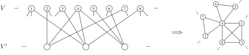
Figure 1: Construction of G(n) from
A(n).
share a P(AiBj/(µn)) number of edges (see Remark 2.1). Conditioned on the weights of
vertices, i.e. on ω, the numbers of edges between distinct pairs of vertices are independent and there is no edge in A(n) connecting vertices either both inV(n) or both in V0(n). Note
that in A(n), the degree of vertex v
i ∈V(n) isP(A
(n)
i ) with
A(in) =AiL0(n)/(µn) a.s.
−−→Ai as n→ ∞, (2.3)
while the degree of vertex v0
j ∈V0(n) is P(B
(n)
j ) with
Bj(n) =BjL(n)/(µn) a.s.
−−→Bj asn → ∞. (2.4)
The random variables A(n) and B(n) are defined by
P(A(n)≤x) = n−1|{1≤i≤n:A(in)≤x}|, (x≥0) and (2.5)
P(B(n)≤x) = bαnc−1|{1≤j ≤ bαnc:Bj(n) ≤x}|, (x≥0). (2.6)
Thus, A(n)(ω) and B(n)(ω) are random variables with the empirical distribution of the
rescaled weights {A(in)} and {B(jn)}, respectively. By the strong law of large numbers, A(n) ⇒A and B(n)⇒B as n→ ∞.
For the purpose of this paper it is not important how the graphs in the sequence depend on each other. For simplicity we assume that, conditioned onω = (Ai, i∈N)×(Bj, j ∈N),
the graphs (A(n), n ∈N) are independent.
The vertices of the random intersection graph G(n) are precisely those in V(n). Two
(distinct) vertices share an edge in G(n) if and only if there is at least one path of length
2 between them in A(n). Thus, G(n) is a simple graph. This construction is visualised
in Figure 1. We note that G(n) is slightly different from an ordinary random intersection
graph. In [11, 14] the conditional probability that vertices with weights Ai and Bj share
an edge in A(n) is given by min(1, AiBj/(µn)), as opposed to 1−exp[−AiBj/(µn)] in this
paper. (Note also that in [11] the weights are constant.)
Remark 2.1. Of course it is possible to construct a simple version of the (multi) graphA(n)
directly, in which the vertices vi andv0j share an edge with probability 1−exp[−AiBj/(µn)].
Indeed, this is sufficient to describe the population structure of our model. We use the present construction, where vi andvj share a Poisson distributed number of edges, in order
Remark 2.2. The graph G(n) is a graph of overlapping cliques, in which, asymptotically
as n → ∞, the number of cliques a vertex is part of has an MP(A) distribution and the clique sizes have an MP(B) distribution. Both of these distributions have finite mean by assumption.
Remark 2.3. Since the random intersection graph does not change if, for somer ∈(0,∞), the random variables AandB are replaced byrAandB/r, condition (2.2) might be replaced by E[A] < ∞ and E[B] < ∞ but this does not gain any generality. The linear scaling
|V0(n)|=bα|V(n)|cis assumed in order to guarantee that, as n → ∞, (i) clique sizes do not
grow to infinity, and (ii) two (or more) cliques contain at most one common vertex, with high probability.
Remark 2.4. In this paper we make use of the following equivalent way of constructing
A(n). Initially all vertices are unexplored. Pick a vertex from V(n) according to some law
(e.g. uniformly at random), say vertex vi, which has weight Ai; this vertex becomes active.
Assign a P(A(in))number of edges to it (see (2.3)). The end-vertices inV0(n) of these edges
are chosen independently with replacement and the probability that v0
j is chosen is Bj/L0(n).
After this vertex vi is made explored, while the chosen vertices become active.
Now, if there are any, explore the active vertices fromV0(n) one by one. Suppose that we
explore vertex v0
j, which has weight Bj; then assign a P(B
(n)
j ) number of edges to it. (We
observe that the number of edges between v0
j and a previously unexplored vertexvl is indeed
P(AlBj/(µn)), independent of the numbers of edges between all other pairs of vertices, as
desired.) These edges connect to vertices chosen independently, with replacement, from V(n); vertex v
l being chosen with probability Al/L(n). If the end vertex has already been
explored then the edge is ignored and not added to the graph, otherwise it is added and the end vertex in V(n) becomes active. If all the edges from v0
j are drawn, then v0j is made
explored.
The next step is to pick one of the active vertices from V(n), if there are any, according
to some, for now unspecified, law and explore it. Say that we choose vk, which has weight
Ak. Then we proceed as in the first step. We assign a P(A
(n)
k ) number of edges to it, then
the end-vertices in V0(n) of these edges are chosen independently with replacement and the
probability that v0
j is chosen isBj/L0(n). If the end vertex has been explored before, then the
edge is ignored and deleted. After this, vertex vk is made explored and the newly chosen
vertices in V0(n) which are unexplored become active. We now explore all active vertices
in V0(n) in turn, and so on until there is no active vertex left. After that an unexplored
vertex from V(n) is chosen and the process goes on until all vertices in V(n) are explored.
Note that if after this construction there are unexplored vertices left in V0(n), they will have
degree 0, since there is no end-vertex left in V(n) to connect to.
2.3
SIR epidemics
We consider a stochastic SIR epidemic on the random intersection graphG(n). The vertices
at the points of independent Poisson processes of unit intensity. If an infectious individual contacts a susceptible one, the susceptible becomes infectious. Infectious individuals stay infectious for a random infectious period, distributed as a random variable I, after which the infectious individual recovers and plays no further part in the epidemic. Infectious periods are i.i.d. and independent of the Poisson processes generating the contacts. An infectious contact is a contact by an infectious individual, irrespective of the state of the receiving individual. Note that there is no loss of generality in assuming that the intensity of the Poisson processes governing the contacts is 1, since this can always be achieved by rescaling time. We denote the above epidemic model by E(n)(A, B,I).
For ease of exposition, primarily to avoid multitype branching processes that are re-ducible, we assume that P(I = 0) = 0. We omit the details but our results are readily extended to the caseP(I = 0)>0. Note, however, that we do allow for the possibility that
P(I =∞)>0; if an infectious individual has infinite infectious period then, almost surely,
that individual makes infectious contact with every member of each clique it belongs to. In order to study properties of the epidemic on a graph, G say, we introduce the Epi-demic Generated Graph, which is a directed graph constructed as follows. IfGis undirected then make it directed by replacing every edge by two edges connecting the same vertices but in opposite directions. Assign every vertex iinGan independent realisation,xi, of the
random variable I. Now thin G by deleting, independently, each (directed) edge emanat-ing from vertex i with probability e−xi. Thus an edge starting at v
i is deleted if infection
would not pass along it werevi to become infected during the epidemic. The set of vertices
that can be reached in the Epidemic Generated Graph from an initially infectious vertex v0 (including v0 itself) is distributed as the set of ultimately recovered individuals. The
set of vertices from which there is a path in the Epidemic Generated Graph to vertex v0,
including v0 itself, is said to be the susceptibility set of v0 [3, 5]. If one of the vertices in
the susceptibility set of v0 is the initially infectious individual, then v0 will be ultimately
recovered in the epidemic.
3
Main results and heuristics
3.1
Introduction
random intersection graphs, indexed by the population size n, and proving associated limit theorems. These theorems are stated in Section 3.4 and proved in Section 5. Calculation of extinction probabilities for the forward and backward branching processes requires exact results concerning the final outcome and susceptibility sets for standard SIR epidemics in closed homogeneously mixing populations, which are given in Appendix B.
3.2
Early stages of an epidemic
3.2.1 Fixed infectious period
Consider the epidemic modelE(n)(A, B,I) defined in Section2.3and, for simplicity, suppose
first that the infectious period is constant, i.e. there existsι >0 such thatP(I =ι) = 1. In the limit as the population sizen → ∞, the initial infective,i∗say, belongs toX ∼ MP(A)
cliques, having sizes ˇY1 + 1,Yˇ2 + 1,· · · ,YˇX + 1, where, given X, the random variables
ˇ
Y1,Yˇ2,· · · ,YˇX are mutually independent and ( ˇYi|X) ∼ MP( ˜B) (i = 1,2,· · · , X). The
size biasing comes in because the probability of being part of a clique is proportional to its weight. Moreover, apart from i∗, these cliques are almost surely disjoint as n → ∞. The initial infective will trigger a local (within-clique) epidemic in each of the X cliques it belongs to. The group of initial susceptibles in a single clique that are infected through a local epidemic started by i∗ is called a litter of i∗. (Note that a litter may be empty, i.e. if no susceptible in the corresponding clique is infected.) Let T(m) denote the size of a typical litter, not counting the initial infective i∗, given that the clique has size m+ 1.
(We call T(m) the size of a local epidemic or the size of a litter.) Then the total number of individuals infected (excluding i∗) by the local epidemics in the cliques that i∗ belongs to is distributed as
Cf = X
X
i=1
T( ˇYi),
where T( ˇY1), T( ˇY2),· · · , T( ˇYX) are independent, since the infectious period is constant.
Now consider a typical individual,j∗ say, that is part of one of the litters of i∗. In the
limit as n→ ∞, (i) individualj∗ belongs to ˇX ∼ MP( ˜A) cliques, in addition to the clique
j∗ was infected through (i.e. the one also containing i∗), having sizes distributed indepen-dently as MP( ˜B) + 1 and (ii) apart from j∗, the ˇX+ 1 cliques containing j∗ are disjoint.
(The size biasing here arises because, in the construction of G(n), the probability that a
vertex joins a given clique is proportional to the weight of that vertex; see Remark 2.4.) Individual j∗ will trigger a local epidemic in each of the ˇX ‘new’ cliques it belongs to. The
total number of individuals infected (excluding j∗) in these ˇX local epidemics (the sum of
the sizes of the litters of j∗) is distributed as
˜ Cf =
ˇ
X
X
i=1
T( ˇYi),
where, given ˇX, the random variables T( ˇY1), T( ˇY2),· · · , T( ˇYXˇ) are independent.
process, with one initial ancestor, and offspring distribution distributed as Cf in the initial
generation and as ˜Cf in all subsequent generations. This approximation is made precise
by using a coupling argument in Section 5.1. The coupling between the epidemic and branching processes breaks down when a clique used to spread a local epidemic intersects a previously used clique, which, with probability tending to one asn → ∞, happens if and only if the branching process does not go extinct.
Let
R∗ =E[ ˜Cf] =
EYˇ[E[T( ˇY)|Yˇ]]E[ ˇX] =EYˇ[E[T( ˇY)|Yˇ]]E[ ˜A] (3.1)
and, for s∈[0,1], let
fCf(s) =E[sC f
] =fX(EYˇ[fT( ˇY)|Yˇ(s)])
and
fC˜f(s) = E[s ˜
Cf
] =fXˇ(EYˇ[fT( ˇY)|Yˇ(s)]).
Let ρ be the survival probability of the above branching process (i.e. the probability that it does not go extinct). Then, by standard branching process theory [20, Theorem 2.3.1], if R∗ ≤1 thenρ= 0 and if R∗ >1 then
ρ= 1−fCf(σ), (3.2)
where σ is the unique solution in [0,1) of the equation
fC˜f(s) =s. (3.3)
The coupling of the epidemic and branching processes mentioned above implies that, if the population size n is suitably large, R∗ is a threshold parameter for the epidemic process and the probability that an epidemic initiated by a single infective becomes established and leads to a major outbreak is given approximately by ρ. Note that in [11], the notation R0 is used instead of R∗. We use the notation of [7, 8], because R0 is usually defined as
the expected number of new direct infections caused by an infectious individual in the first stages of an epidemic [2,15, 29], while in (3.1)all individuals infected by a local epidemic are ‘assigned to’ the initial infectious individual in the clique.
3.2.2 General infectious period distribution
When the infectious period is not constant we can still approximate the epidemicE(n)(A, B,I)
by considering successive local epidemics as above, but the approximating process is no longer a simple single-type branching process. There are two reasons for this. First, the sizes of the litters of an individual, i∗ say, are not independent since the infectious period
In view of these observations, we approximate the early stages of the epidemicE(n)(A, B,I)
by a multitype branching process
Zf =Zf(A, B,I) = (Zf
i , i∈Z+),
defined as follows. The type space is (0,∞], with the type of an individual being given by the infectious period of the corresponding individual in the epidemic process. For i∈ Z+, Zif is a multiset of points in (0,∞] giving the types of individuals present in generation i of the branching process. (Note that if the distribution of I has atoms, at infinity or otherwise, then Zif may contain repeated elements; on the other hand if the distribution of I is continuous then, almost surely, all elements of Zif are distinct and hence Zif is a set.) There is one initial ancestor, corresponding to the initial infective, i∗ say, in the epidemic E(n)(A, B,I) and its type is distributed asI. As in the constant infectious period
case, i∗ belongs to X ∼ MP(A) cliques, having sizes distributed independently as ˇY + 1,
where ˇY ∼ MP( ˜B), and in Zf, the offspring of the initial ancestor corresponds to all the
individuals infected in the local epidemics triggered by i∗ in these X cliques, though now
of course we also keep track of their types (infectious periods). In the branching process, a group of children corresponding to a litter in the epidemic process is also referred to as a litter. The offspring of any individuals in a non-initial generation of Zf are defined in a
similar fashion, except X is replaced by ˇX ∼ MP( ˜A). Of course, the offspring of distinct individuals in Zf are mutually independent.
The branching process Zf, which we call a forward branching process because it
ap-proximates the forward spread of the epidemic E(n)(A, B,I), is analysed in Section 4. Let
˜
Zf be the multitype branching process defined analogously to Zf, except the offspring
distribution in all generations of ˜Zf is that of the non-initial generations in Zf. Let ρ be
the probability that Zf survives and, for x ∈ (0,∞], let ˜ρ(x) be the probability that ˜Zf
survives given that the ancestor has type x. Let R∗ be defined as in (3.1), where T(m)
is distributed as the size of a local epidemic, initiated by a single infective in a clique of size m+ 1, in which the infectious periods of infectives (including the initial one) are i.i.d. copies of I. (An expression forEYˇ[E[T( ˇY)|Yˇ]] is given by equation (B.7) in Appendix B.2,
thus enabling R∗ to be computed.) Then ρ > 0 if and only if R∗ > 1 (see Theorem 4.2), so R∗ is still a threshold parameter for the epidemic. Also, when R∗ >1,ρ is given by an infinite-type analogue of (3.2); see (4.2), which expresses ρ as the expectation of a func-tional of ˜ρ with respect to the distribution I of x. Furthermore, ˜ρ satisfies a functional equation (see (4.1)), which is essentially an infinite-type analogue of (3.3) and has at most one non-zero solution (see Lemma 4.1).
3.3
Final outcome of an epidemic
Recall the definition of the susceptibility set of an individual given in Section 2.3. We require also the concept of a local susceptibility set, which is defined in exactly the same way as a susceptibility set but for an epidemic on a single clique. For m = 0,1,· · ·, let S(m) denote the size of a typical local susceptibility set of an individual in a clique of size m+ 1, where S(m) does not include the individual itself.
We may approximate the early growth of a susceptibility set of an individual,i∗ say, by
consider first those individuals, not including i∗ itself, who belong to a local susceptibility set of i∗. These are the offspring ofi∗ in the branching process. We next repeat this process
for each individual, j∗ say, in the first generation of the branching process to obtain the
second generation, and so on. (When determining the offspring ofj∗, we need only consider its local susceptibility set in cliques other than that which containsi∗; any individual inj∗’s
local susceptibility set who is in that clique has already been counted as part of i∗’s local
susceptibility set.) In the limit as n→ ∞, this leads to a (backward) branching process
Zb =Zb(A, B,I) = (Zb
i, i∈Z+)
having one initial ancestor, in which the number of offspring of the ancestor is distributed as
Cb = X
X
i=1
S( ˇYi),
and the number of offspring of any subsequent individual is distributed as
˜ Cb =
ˇ
X
X
i=1
S( ˇYi),
where X,X,ˇ Yˇ1,Yˇ2,· · · are independent, X ∼ MP(A), ˇX ∼ MP( ˜A) and ˇYi ∼ MP( ˜B)
(i= 1,2,· · ·).
Note that the local susceptibility set of an individual is independent of its infectious period, so Zb is a single-type branching process; thus Zb
i is determined by its cardinality
|Zb
i|, in contrast to Z f
i (which is single-type only if I is almost surely equal to a fixed
constant). Let
Rb
∗ =E[ ˜Cb] =EYˇ[E[S( ˇY)|Yˇ]]E[ ˜A] (3.4)
be the mean number of children of an individual in Zb who is not the ancestor and, for
s ∈[0,1], define the probability generating functions
fCb(s) = E[sC b
] =fX(EYˇ[fS( ˇY)|Yˇ(s)])
and
fC˜b(s) =E[s ˜
Cb
] =fXˇ(EYˇ[fS( ˇY)|Yˇ(s)]).
Denote by ρb = ρb(A, B,I) the survival probability of Zb. Then, by standard branching
process theory, if Rb
∗ ≤1 then ρb = 0 and if Rb∗ >1 then
ρb = 1−f
Cb(ξ), (3.5)
where ξ is the unique solution in [0,1) of the equation
fC˜b(s) =s.
Note that an expression for EYˇ[fS( ˇY)|Yˇ(s)] is given by equation (B.8) in Appendix B.2,
fX(s) = φA(1−s) and observe that fXˇ(s) = φA˜(1−s) = −φ0A(1−s)/E[A], where φ0A is
the derivative of φA.
Before describing how the backward branching process Zb is used to study the final
outcome of an epidemic in a large population, we discuss briefly the relationship between the forward and backward branching processes. In particular we note two important con-sequences of this relationship.
Remark 3.1. Let G0 be the Epidemic Generated Graph (see Section 2.3) for an epidemic
on a single clique (G say) of m+ 1 individuals, labelled 0,1,· · · , m. For distinct i, j ∈ {0,1,· · ·, m}, let χi,j = 1 if there is a chain of directed edges from i to j in G0 and
let χi,j = 0 otherwise. Then T(m) and S(m) are distributed as
Pm
i=1χ0,i and
Pm
i=1χi,0,
respectively, so by symmetry, E[T(m)] = mP(χ0,1 = 1) and E[S(m)] = mP(χ1,0 = 1).
Further, by symmetry, P(χ0,1 = 1) =P(χ1,0 = 1), and it follows from (3.1) and (3.4) that
Rb
∗ =R∗. Thus we use only the notation R∗.
Remark 3.2. Consider the graphs G andG0 of the previous remark, and suppose that the
infectious period I is constant, say P(I = ι) = 1. Then G0 is obtained from the directed version of G by deleting directed edges independently, each with probability e−ι. Thus,
if G00 is obtained from G0 by reversing the direction of all arrows, then G00 and G0 are
identically distributed, whence so are T(m) and S(m). It follows that in this case ρb = ρ.
This argument breaks down when I is not constant. In that case, apart from the branching process Zf being multitype, the presence/absence of directed edges from a given vertex inG0
are not independent, whence T(m) and S(m) have different distributions. Thus generally ρb 6=ρ.
Now we describe informally the relationship between the backward branching process and the final outcome of an epidemic. (This description assumes that there is no vertex with weight greater than logn; the full argument is given in Section 5.2.) Consider the epidemic model E(n)(A, B,I) and suppose that the population size n is large. Choose
an initially susceptible individual uniformly at random from all initial susceptibles, j say, and construct its susceptibility set on a generation basis as described above for Zb. Stop
this construction after tn = dlog logne generations or when the susceptibility set process
goes extinct, whichever occurs first. The susceptibility set process can be coupled to the backward branching process Zb so that, with probability tending to 1 asn → ∞, the two
coincide over generations 0,1,· · · , tn and their common size at generationtnis not greater
than n for any >0 (cf. the start of the proof of Lemma 5.8). Also, ifR
∗ >1, there exists
c > 0 such that the probability thatZb
tn >(logn)
c tends to ρb as n→ ∞ (cf. Lemma 5.8).
By symmetry, the initial infective in E(n)(A, B,I),i say, may be chosen by picking an
individual uniformly at random from the population excluding j. Thus, if j’s suscepti-bility set process goes extinct before reaching generation tn then the probability that j’s
susceptibility set contains the initial infective (and hence that j is ultimately infected by the epidemic) tends to zero as n → ∞. Suppose instead that j’s susceptibility set process does reach generation tn. Then we choose the initial infective i as above, construct the
forward epidemic process from iand determine whether or not the latter intersects the (at least (logn)c and at most n) individuals in generation t
n of j’s partially constructed
Recall that the forward epidemic process originating from i is approximated by the branching processZf. IfZf goes extinct then, in the limit asn → ∞, there are only finitely
many individuals infected in the epidemic and hence the probability that the epidemic intersects generation tn of j’s partially constructed susceptibility set tends to zero. If Zf
does not go extinct then, by exploiting a lower bounding branching process for the epidemic process, we show in Section 5.2that, as n→ ∞, the epidemic process almost surely infects Θ(n) individuals and hence the probability that it intersects generation tn of j’s partially
constructed susceptibility set tends to one.
The above implies that the asymptotic probability that an initial susceptible, chosen uniformly at random, is ultimately infected by a major outbreak isρb. Hence the asymptotic
expected proportion of the population ultimately infected by a major outbreak is also ρb.
Now consider two distinct initial susceptibles chosen uniformly at random, j1 and j2 say,
and construct their susceptibility sets on a generation basis as above, stopping each process after tn generations or if it goes extinct. The two partially constructed susceptibility set
processes are asymptotically independent as n → ∞, which enables a weak law of large numbers to be proved for the proportion of the population that is ultimately infected by a major outbreak.
3.4
Limit theorems for SIR epidemics on random intersection
graphs
Let R(n) = R(n)(A, B,I) be the set of ultimately recovered vertices, including the
sin-gle initial infective, in the SIR epidemic E(n)(A, B,I) on the random intersection graph
G(n), constructed using the infectious period distribution I and the sequences (A
i, i∈N),
(Bj, j ∈N) (as described in Section2.2). Our focus is on the properties of|R(n)|, the
num-ber of ultimately recovered individuals in the epidemic. For a branching process,Zf say, let
|Zf|=P∞
i=0|Z
f
i | denote its total size (total progeny), including the ancestor. Recall that
Zf = Zf(A, B,I) and Zb = Zb(A, B,I) are the (forward and backward) branching
pro-cesses, which approximate the epidemic process and the process exploring a susceptibility set, respectively. Recall also that ρ and ρb are their respective survival probabilities.
Our first theorem establishes the precise sense in which the forward process approxi-mates the early stages of an epidemic.
Theorem 3.3. For all k∈N,
lim
n→∞P(|R
(n)|
=k) = P(|Zf|=k).
The next result establishes the connection between the backward process and the pro-portion of individuals ultimately infected.
Theorem 3.4. Suppose that R∗ >1. Then for every 0< < ρb,
lim
n→∞P
|R(n)|
n −ρ
b
<
=ρ.
Theorem 3.5. Let TF be a random variable with P(TF =ρb) = ρ= 1−P(TF = 0). Then,
as n→ ∞,
n−1|R(n)| ⇒T
F.
Proof. First note that Theorem 3.3 implies that, for any >0 and any k∈N,
lim inf
n→∞ P n
−1|R(n)| ≤
≥P(|Zf| ≤k),
whence, letting k → ∞,
lim inf
n→∞ P n
−1|R(n)| ≤
≥1−ρ. (3.6)
Suppose that R∗ ≤1. Then ρ= 0 and (3.6) implies that
n−1|R(n)| ⇒0 asn → ∞. (3.7)
On the other hand, suppose that R∗ >1, so ρ >0 and ρb >0. Then Theorem 3.4 implies
that, for 0 < < ρb, lim sup
n→∞P n−1|R(n)| ≤
≤ 1−ρ, which, together with (3.6), yields that, for such ,
lim
n→∞P n
−1|R(n)| ≤
= 1−ρ.
The theorem then follows upon combining this observation with (3.7) and Theorem3.4.
4
Properties of the forward branching process
In this section we study the survival probability of the branching process Zf introduced
in Section 3.2. Recall that individuals in Zf are typed by the length of the infectious
period of the corresponding individual in the epidemic process. There is one ancestor, i∗ say, whose type is distributed as I and who belongs to X ∼ MP(A) cliques. (That is, the corresponding individual in the epidemic processE(n)(A, B,I) belongs toX ∼ MP(A)
cliques.) Those cliques have sizes that are independent and identically distributed as 1 + ˇY, where ˇY ∼ MP( ˜B). The offspring of the ancestor correspond to the individuals who, in the corresponding epidemic process, are infected by the local epidemics triggered by i∗ in
the X cliques it belongs to. The offspring of i∗ are grouped into litters with each litter corresponding to a clique ofi∗. Note that some litters might be empty (if the epidemic fails
to spread further into some cliques to which i∗ belongs). The offspring of any subsequent
individual is defined similarly, except that such an individual belongs to ˇX ∼ MP( ˜A) cliques in addition to the clique it was infected through. The type space for Zf is given
by the support of I, which for ease of exposition we assume is (0,∞]. Extension to cases where I is supported on a proper subset of (0,∞] is straightforward.
We investigate the survival probability of Zf using functionals defined on measurable
test functions h: (0,∞] →[0,1] as follows (cf. [9, 10]). Let h(x) be a given test function. Suppose that individuals in Zf are marked independently, with an individual of type x
function of X is given by fX(s) = φA(1−s) (s ∈ [0,1]), where φA(θ) = E[e−θA] is the
moment generating function of A. It follows that
Φ(h)(x) = 1−φA(F(h)(x)).
Define the functional ˜Φ(h)(x) similarly for the branching process ˜Zf, defined in the final
paragraph of Section 3.2.2; thus
˜
Φ(h)(x) = 1−φA˜(F(h)(x)).
Let ρi be the probability that generation i of the branching process Zf is non-empty,
that is ρi = P(|Zif| > 0). By definition ρi is non-increasing, so ρ = limi→∞ρi exists
and is the probability of survival of the branching process. Let ˜ρi(x) be the probability
that the lineage of an individual (i.e. the sub-process consisting of that individual and all its descendants), which is not the ancestor and has type x, survives for at least i further generations and let ˜ρ(x) = limi→∞ρ˜i(x) be the probability that this lineage survives forever.
Note that ˜ρ1(x) = ˜Φ(1)(x), where1is the function which is equal to 1 on its entire domain.
It is clear that ˜ρ(x) satisfies
˜
ρ(x) = ˜Φ( ˜ρ)(x), (4.1)
since in order for the lineage of an individual to survive, at least one of the children of that individual must have a surviving lineage. Furthermore,
ρ= Z
(0,∞]
Φ( ˜ρ)(x)P(I ∈dx) = E[Φ( ˜ρ)(I)]. (4.2)
Let ˜Φi be the i-th iterate of ˜Φ and note that ˜ρi(x) = ˜Φi(1)(x). The functionals Φ(h)(x)
and ˜Φ(h)(x) are monotonic increasing in h (e.g. if h1(x) ≥ h2(x) for all x ∈ (0,∞] then
Φ(h1)(x)≥Φ(h2)(x) for allx∈(0,∞]). Therefore, ˜ρ(x) = limi→∞Φ˜i(1)(x) is the pointwise
maximal solution of (4.1). Note that, since Zf is irreducible, either ˜ρ(x) = 0 for all
x ∈(0,∞] or ˜ρ(x)>0 for all x∈(0,∞]. The following lemma is proved and discussed in Appendix A.
Lemma 4.1. There is at most one non-zero solution ρ(x)˜ of (4.1).
Now recall the definition ofR∗ from (3.1), where ˇY ∼ MP( ˜B) and as before letT(m) denote the size of a litter, in a clique ofminitial susceptibles, in which the infectious periods of infectives are i.i.d. copies of I. It is convenient here to show explicitly the dependence on I and write T(m) =T(m,I), so
R∗ =EYˇ[E[T( ˇY ,I)|Yˇ]]E[ ˜A].
Theorem 4.2. The survival probability satisfies ρ >0 if and only if R∗ >1.
Proof. Suppose first that R∗ >1. Fork ∈Z+, letL(k,I) = E[T( ˇY ,I)|Yˇ =k]. Then there
exists K ∈N such that
E[ ˜A]
K
X
k=0
For >0, letI be the discrete random variable obtained from I byI =bI/c(with
the convention that b∞c = ∞) and note that I is stochastically smaller than I. Since
L(k,I) depends on the realisation of an Epidemic Generated Graph defined on a finite clique, there exists >0 such that
E[ ˜A]
K
X
k=0
L(k,I)P( ˇY =k)>1.
Analagously to the derivation of (4.3), there exists K0
∈ N such that for I0 = I1(1I 6∈
(K0
,∞)), we have
E[ ˜A]
K
X
k=0
L(k,I0)P( ˇY =k)>1. (4.4)
Consider the branching process ˜Zf(A, B,I0
), which has finitely many types and is
irreducible. Let ˜M be the mean offspring matrix of ˜Zf(A, B,I0
). Note that whether or
not an individual in a clique becomes infected is independent of that individual’s own infectious period. It follows that the rows of ˜M are each proportional to the probability mass function of I0
, so ˜M has rank one and the maximal eigenvalue of ˜M is given by its
trace, which is easily seen to be equal to the left hand side of (4.4) with K replaced by ∞. Therefore, if R∗ > 1, the branching process ˜Zf(A, B,I) dominates the irreducible
finite-type supercritical branching process ˜Zf(A, B,I0
), which we know from standard theory [20,
Theorem 4.2.2] has a strictly positive probability of survival. Thus ˜ρ(x) > 0 for all x ∈
(0,∞]; equation (4.2) then implies that ρ >0.
ForR∗ ≤1 we use a similar argument to [10]. Suppose thatR∗ ≤1 and that ˜ρ(x)>0 for some (and thus all) x∈(0,∞]. Recall that ˜Φ( ˜ρ)(x) is the probability that, in ˜Zf(A, B,I)
and with individuals of type x being marked with probability ˜ρ(x), an individual of type x has at least one marked child. Note that this probability is strictly smaller than the expectation of the number, TM(x,ρ) say, of marked children of such an individual. Let˜
T(x, m,I) denote the size of a single-clique epidemic with m initial susceptibles and a single initial infective which has infectious period x. Then, again exploiting the fact that whether or not an individual is infected is independent of its infectious period, we find that
E[TM(x,ρ)] =˜ E[ ˜A]EYˇ[E[T(x,Y ,ˇ I)|Yˇ]]E[ ˜ρ(I)],
whence, recalling (4.1),
˜
ρ(x) = ˜Φ( ˜ρ)(x)<E[ ˜A]EYˇ[E[T(x,Y ,ˇ I)|Yˇ]]E[ ˜ρ(I)]. (4.5)
Note that if x is a realisation of a random variable I0 that is distributed as I, then
E[T(m,I)] = EI0[E[T(I0, m,I)|I0]] and (4.5) implies that E[ ˜ρ(I)] < R∗E[ ˜ρ(I)]. It then
follows that R∗ >1, which is a contradiction. Thus, ifR∗ ≤1 then ˜ρ(x) is identically zero on the support of I and it then follows from (4.2) that ρ= 0.
5
Proofs
infinite sequences (Ai, i ∈N) and (Bj, j ∈ N) and ν is the appropriate (product) measure
determined by the distributions of A and B. In the proofs we consider processes which depend on ω ∈ Ω, that is on the sequences (Ai, i ∈ N) and (Bi, i ∈ N). The measure
governing a process conditioned on ω is denoted by Pω and the corresponding expectation
by Eω. We use the notation Xn pν −−−→
n→∞ X to denote that Xn converges in probability to
X as n → ∞, with respect to the measure ν. That is, Xn pν −−−→
n→∞ X means that for every
>0,δ >0, we haveν(|Xn−X|> )< δ for all sufficiently largen ∈N. In particular, we
often use the notation Pω(Xn ∈ A) pν −−−→
n→∞ P(X∈ A), which is to be interpreted as meaning
that, for a subset A of the state space of Xn and X, we have that for every >0,
Z
ω∈Ω
1
1(|Pω(Xn∈ A)−P(X ∈ A)|> )ν(dω)→0 as n→ ∞.
Additionally, we use the notation Xn = Opν(g(n)) if there exists a constant C > 0 such that Pω(Xn< Cg(n))
pν −−−→
n→∞ 1 andXn= Θpν(g(n)) if there exist constants 0< c < C such
that Pω(cg(n)< Xn < Cg(n)) pν −−−→
n→∞ 1.
We prove the following conditioned versions of Theorems3.3and3.4, in whichR(n)(ω,I)
denotes the set of ultimately recovered vertices, including the single initial infective, in an SIR epidemic (as defined in Section2.3) on the random intersection graphG(n), constructed
using the infectious period distributionI and the sequences (Ai, i∈N), (Bj, j ∈N) denoted
by ω∈Ω.
Theorem 5.1. For k ∈N, we have
Pω(|R(n)(ω,I)|=k) pν −−−→
n→∞ P(|Z
f(A, B,I)|=k).
Theorem 5.2. Suppose that R∗ >1. Then for every 0< < ρb(A, B,I),
Pω
n−1|R(n)(ω,I)| −ρb(A, B,I) <
pν
−−−→
n→∞ ρ(A, B,I).
Proofs of Theorems 3.3 and 3.4. Note that, for fixed k ∈N, the sequence of random vari-ables (Pω(|R(n)(ω,I)| =k), n∈ N) is uniformly integrable, so Theorem 3.3 follows
imme-diately from Theorem 5.1 (and [18, Theorem 7.10.3]), by taking expectations with respect to the measure ν. Theorem 3.4 follows similarly from Theorem 5.2.
5.1
Proof of Theorem
5.1
In this proof we use three processes,
• the branching process Zf =Zf(A, B,I),
• the branching process Z(n) =Zf(A(n), B(n),I), defined similarly to Zf(A, B,I) but
with A and B replaced respectively by A(n) and B(n), defined in (2.5) and (2.6),
• the exploration process of the Epidemic Generated Graph onG(n), denoted byR(n)= R(n)(ω,I) = (R(n)
In the exploration process, R(0n) denotes the initially infective vertex v0, R (n)
1 denotes the
subset of vertices inV(n)\E(n)
0 that in the Epidemic Generated Graph have an edge to them
from v0, R (n)
2 denotes the subset of vertices in V(n)\(R (n)
0 ∪ R
(n)
1 ) that in the Epidemic
Generated Graph have an edge to them from at least one member ofR(1n), and so on. With slight abuse of notation we now use R(n) for the exploration process, where previously it
was the set of ultimately recovered vertices in E(n). As with the branching process Zf,
|R(n)|=P∞
i=0|R (n)
i |is the total number of ultimately recovered vertices; note that this has
precisely the same meaning as in Section 3.4.
To prove Theorem5.1 we first show that the distribution of the total size ofZ(n) is
ap-proximately that of Zf, then that the distribution of the total size ofR(n) is approximately
that of Z(n).
Lemma 5.3. For k ∈N, it holds that Pω(|Z(n)|=k) pν −−−→
n→∞ P(|Z
f|=k).
Proof. Recall that a litter in a branching process is a group of children corresponding with the number of individuals infected in a local epidemic in one clique, excluding the initial susceptible. Let the total number of (possibly empty) litters in Zf and Z(n) be
denoted by H and H(n), respectively. Note that, using [18, Theorem 7.2.19], if X
n ⇒ X,
then MP(Xn) ⇒ MP(X). Recall further that A(n) ⇒ A and B(n) ⇒ B as n → ∞.
These latter convergence results also hold for the size-biased variants, as shown just below equation (2.1). It follows that, as n → ∞, the number and sizes of litters spawned by a typical individual in Z(n) converge in distribution to those of a corresponding typical
individual in Zf. Hence, fork ∈
N and l ∈Z+,
Pω(|Z(n)|=k, H(n) =l) pν −−−→
n→∞ P(|Z
f|=k, H =l).
Therefore, for every l∈N, we have
Pω(|Z(n)|=k, H(n)≤l) pν −−−→
n→∞ P(|Z
f|=k, H ≤l). (5.1)
Note that
Pω(|Z(n)|=k) =Pω(|Z(n)|=k, H(n)≤l) +Pω(|Z(n)|=k, H(n)> l) (5.2)
and
P(|Zf|=k) = P(|Zf|=k, H ≤l) +P(|Zf|=k, H > l).
Fix k ∈ N and > 0. Let Hk be the total number of litters spawned by the first k
vertices evaluated in the branching process Zf, so H
k is distributed as X0 + ˇX1 + ˇX2+ · · ·+ ˇXk−1, whereX0,Xˇ1,Xˇ2,· · · ,Xˇk−1 are independent, X0 ∼ MP(A) and ˇXi ∼ MP( ˜A)
(i= 1,2,· · · , k−1). Now, for any l∈Z+,
P(|Zf|=k, H > l) =P(|Zf|=k, Hk > l)≤P(Hk > l).
Further, Hk is a proper random variable, so P(Hk > l) ↓ 0 as l → ∞. Thus, there exists
L=L(k, )∈N, such that for all l > L,
LetHk(n) be the total number of litters in the first k vertices evaluated in the branching process Z(n). Then, H(n)
k ⇒ Hk, since MP(A
(n)) ⇒ MP(A) and MP( ˜A(n))⇒ MP( ˜A),
whence Pω(H(n) > l) pν −−−→
n→∞ P(H > l), for any l ∈ Z+. Arguing similarly to above and
recalling (5.2), it follows that, given any δ >0, there exists L0 =L0(k, , δ)∈N, such that
for all l > L0,
νPω(|Z(n)|=k)<Pω(|Z(n)|=k, H(n)≤l) +/3
>1−δ/2 (5.4)
for all sufficiently large n.
Fixδ >0 and choose l >max(L, L0). Then (5.1) implies that
νPω(|Z(n)|=k, H(n)≤l)−P(|Zf|=k, H ≤l)< /3
>1−δ/2, (5.5)
for all sufficiently large n. Using the triangle inequality, we obtain
Pω(|Z(n)|=k)−P(|Zf|=k)
≤
Pω(|Z(n)|=k)−Pω(|Z(n)|=k, H(n) ≤l)
+Pω(|Z(n)|=k, H(n) ≤l)−P(|Zf|=k, H ≤l)
+P(|Zf|=k)−P(|Zf|=k, H ≤l) ,
whence, noting that the final term is independent of ω,
νPω(|Z(n)|=k)−P(|Zf|=k)
≥
≤νPω(|Z(n)|=k)≥Pω(|Z(n)|=k, H(n) ≤l) +/3
+ν
Pω(|Z(n)|=k, H(n) ≤l)−P(|Zf|=k, H ≤l)≥/3
+ 11
P(|Zf|=k)≥P(|Zf|=k, H ≤l) +/3
.
By choosing l large enough, it follows, using (5.3), (5.4) and (5.5), that for all sufficiently large n,
ν
Pω(|Z(n)|=k)−P(|Zf|=k)
≥
≤δ/2 +δ/2 + 0 =δ
and the lemma then follows.
Lemma 5.4. For k ∈N, Pω(|Z(n)| ≤k)−Pω(|R(n)| ≤k) pν −−−→
n→∞ 0.
Proof. The proof follows from a standard coupling argument, described below. Firstly though, for each n ∈ N, let v0(n) be a vertex chosen uniformly at random from V(n) and
let v(1n), v (n)
2 ,· · · be independently chosen vertices from V(n), where the probability that a
given vertex is chosen is proportional to itsA-weight. Leta(0n), a (n)
1 ,· · · be the respective
A-weights of v0(n), v (n)
1 ,· · ·. Let I (n)
0 be the type assigned to vertexv (n)
0 . Let v0 (n) 1 , v0
(n)
2 ,· · · be
independently chosen vertices (representing cliques) from V0(n) where the probability that
a given vertex is chosen is proportional to its B-weight. The B-weights of v10(n), v0 (n) 2 ,· · ·
are denoted by b(1n), b (n)
2 ,· · ·, respectively. Let the random variable
T(n) = min(i∈
N:vi(n)=v
(n)
be the smallest index at which a vertex fromV(n)is chosen a second time. Similarly, define
T0(n)= min(i∈
N:vi0(n) =v
0(n)
j for some j < i).
The constructions ofZ(n) and R(n) are coupled as follows. The ancestor ofZ(n) spawns
a P(a(0n)) number of (possibly empty) litters, l0 say. The cliques that the initial infective
in R(n) belongs to are given by v0(n) 1 , v0
(n)
2 ,· · · , v0 (n)
l0 , which might contain duplicates;
the B-weights associated with these litters are b(1n), b (n)
2 ,· · · , b (n)
l0 . If T0(n) > l0, then there
are no duplicates amongst v10(n), v20(n),· · · , vl0(0n) and the processes stay coupled. If not, the
construction can be continued but the details are not important for our purposes.
If the coupling continues the sizes of the litters (recall that litters are defined both for the epidemic process and the branching process) are then determined. For each i= 1,2,· · · , l0,
the size of litteri is distributed as the number of initially susceptible individuals which are ultimately infected by a local epidemic in a group with one initially infectious individual, having infectious period I0(n), and a P(b(in)) distributed number of initially susceptible individuals. The litter sizes are all independent. Say that the total number of vertices in the l0 litters is l, then they get A-weights a(1n), a
(n)
2 ,· · · , a (n)
l and types I
(n) 1 ,I
(n)
2 ,· · · ,I (n)
l ,
which are i.i.d. and distributed as I. If l < T(n) the coupling continues and the generation
1 vertices are v1(n), v2(n),· · · , vl(n). The coupling now proceeds in the obvious way. Note that in this construction we have not yet decided which vertices are in the same clique (of the random intersection graph) as v(1n) but are not infected by the local epidemic.
Let H(n) be as in the proof of Lemma 5.3 and let H(∗n) be the corresponding number
for R(n). We need to prove that fork ∈
N and l∈Z+,
Pω(|Z(n)|=k, H(n) =l)−Pω(|R(n)|=k, H(∗n) =l) pν −−−→
n→∞ 0,
and then deduce the statement of the lemma as in the latter part of the proof of Lemma5.3. Note that the coupling gives
Pω(|Z(n)|=k, H(n)=l, T(n) > k, T0(n)> l) (5.6)
=Pω(|R(n)|=k, H(∗n)=l, T(n)> k, T0(n) > l).
Furthermore, letting C(n)(k, l) ={T(n)≤k} ∪ {T0(n)≤l}, we have
Pω(|Z(n)|=k, H(n)=l) = Pω(|Z(n)|=k, H(n) =l, T(n)> k, T0(n) > l)
+ Pω(|Z(n)|=k, H(n) =l, C(n)(k, l)).
Note that the second term on the right hand side of this expression is bounded above by
Pω(C(n)(k, l)).
Recall from Section 2.2 that µ = E[A] = αE[B] < ∞, which implies that the total
weight of vertices in V(n) with weight exceeding logn is ν-almost surely o(n). (To show
this, note that, since µ < ∞, for anyN >0,
n−1
n
X
i=1
Ai1(A1 i > N) a.s.
and E[A11(A > N)]→0 asN → ∞.) A similar result holds for the weights of the vertices in V0(n). Hence, for every k, l∈
N, the probability that both max(a(in) : 0≤i≤k)≤logn
and max(b(jn) : 1 ≤ j ≤ l) ≤ logn converges to 1 as n → ∞. Thus, the total weight of the first k vertices and the firstl litters chosen in the branching process is ν-almost surely O(logn). By a birthday problem argument we deduce that Pω(C(n)(l, k))
pν −−−→
n→∞ 0. (Note
that if Mn(k) is the number of distinct pairs (i, j) with 0≤i < j ≤k and v(in)=v
(n)
j , then
under the above restrictions, Eω[Mn(k)]≤ k(k−1)
2 logn L(n)
pν −−−→
n→∞ 0). Thus, for every k, l∈N,
Pω(|Z(n)|=k, H(n)=l)−Pω(|Z(n)|=k, H(n)=l, T(n) > k, T0(n)> l) pν −−−→
n→∞ 0.
Similarly, we deduce that, again for all k, l∈N,
Pω(|R(n)|=k, H(∗n)=l)−Pω(|R(n)|=k, H(∗n) =l, T(n) > k, T0(n) > l) pν −−−→
n→∞ 0;
which, together with (5.6), yields the lemma.
Theorem 5.1 follows immediately by combining Lemmas 5.3 and 5.4.
5.2
Proof of Theorem
5.2
Before considering susceptibility sets and backward branching processes, we prove the fol-lowing extension of Lemma 5.3 which is required later in this section.
Lemma 5.5. ρ(A(n), B(n),I) pν −−−→
n→∞ ρ(A, B,I).
Proof. For every k ∈Z+, define the random variable
Ik(I) =
2−kb2kIc if I <2k, 2k if I ∈[2k,∞),
∞ if I =∞.
That is, Ik is a random variable which can take only finitely many values and for j =
0,1,· · · ,4k−1,
P(Ik =j2−k) =P I ∈[j2−k,(j+ 1)2−k),
while P(Ik = 2k) =
P(I ∈[2k,∞)) and P(Ik = ∞) =P(I =∞). It is clear that Ik ⇒ I
as k → ∞and that Ik is stochastically smaller than Ik+1 for all k ∈
Z+.
For non-negative random variablesX and Y, the function ˜ρ(X, Y,Ik) is pointwise
non-decreasing in k, since it is the survival probability of a branching process and (stochasti-cally) increasing the distribution of the infectious periods, and thus also of the offspring distribution, cannot decrease the survival probability of the process. By monotonicity we have that limk→∞ρ(X, Y,˜ Ik) exists pointwise, and by the monotone convergence theorem
this limit satisfies (4.1) for ˜ρ(X, Y,I). By Lemma 5.3 we know that for every k ∈ N,
Pω(|Z(n)|> k) pν −−−→
n→∞ P(|Z
f|> k). This implies that for every >0 and δ >0, there exists
N0 ∈N such that for n > N0, we have
ν ρ(A(n), B(n),I)< ρ(A, B,I) +
Furthermore, for every >0, there exists K ∈N such that fork > K, we have
ρ(A, B,Ik)> ρ(A, B,I)−/2.
Similarly, for every > 0, δ > 0 and k ∈N, there exist Nk ∈ N such that for n > Nk, we
have
ν ρ(A(n), B(n),Ik)> ρ(A, B,Ik)−/2
>1−δ/2,
while for every k ∈ N (and ω ∈ Ω), ρ(A(n), B(n),I) ≥ ρ(A(n), B(n),Ik). Combining these
statements establishes that, for every >0 andδ >0, there exists N ∈Nsuch that for all n > N, we have
ν ρ(A(n), B(n),I)> ρ(A, B,I)−
>1−δ/2.
Combining this with (5.7) completes the proof of the lemma.
In order to prove Theorem 5.2, we investigate the susceptibility sets of two vertices chosen uniformly at random in the subgraph ˆG(n) (ofG(n)), which is defined as follows. Let
ˆ
A(n) be constructed from A(n) by ignoring all vertices in V(n) and V0(n) that have weights
larger than logn and ignoring all edges that are incident to such vertices. The graph ˆG(n)
is constructed from ˆA(n) in the same way that G(n) is constructed from
A(n).
We can create a realisation of ˆA(n) as follows. Define the vertex sets ˆV(n) = (v
i ∈V(n):
Ai ≤ logn) and ˆV0(n) = (vj0 ∈ V0(n) : Bj ≤ logn). Conditional upon the weights of the
vertices in A(n), (i) vertices v
i ∈Vˆ(n) and vj0 ∈Vˆ0(n) share in ˆA(n) aP(AiBj/(µn)) number
of edges and (ii) the number of edges between distinct pairs of vertices are independent. Let
ˆ
L(n)= X
i:vi∈Vˆ(n)
Ai and
ˆ
L0(n)= X
j:v0j∈Vˆ0(n)
Bj.
Then the degree of vertexvi ∈Vˆ(n)in ˆA(n) isP(AiLˆ0(n)/(µn)) and the degree ofvj0 ∈Vˆ0(n)is
P(BjLˆ(n)/(µn)). We construct from ˆA(n) an identically distributed copy of A(n) by adding
the vertices fromV(n)\Vˆ(n)andV0(n)\Vˆ0(n) and, ifv
i ∈V(n) andv0j ∈V0(n)are not both in
ˆ
A(n), letting vi and vj0 share a P(AiBj/(µn)) number of newly-added edges, independently
of the number of edges between other vertices.
We construct a coupling of two independent branching processes and the susceptibility sets of v1 and v2 in ˆG(n) (which by exchangeability is equivalent to choosing two distinct
vertices uniformly at random), assuming thatA1, A2 ≤logn. We therefore define (cf.
equa-tions (2.3)–(2.6)) ˆA(in) =Ai1(A1 i ≤logn) ˆL0(n)/(µn) and ˆB
(n)
i =Bi1(B1 i ≤ logn) ˆL(n)/(µn);
and let ˆc(An) = Pn
i=11(A1 i ≤ logn) and ˆc
(n)
B =
Pbαnc
i=1 1(B1 i ≤ logn). The random variables
ˆ
A(n) and ˆB(n) are defined by
Pω( ˆA(n)≤x) = |{1≤i≤ˆc
(n)
A : ˆA
(n)
i ≤x}|/ˆc
(n)
A (x≥0) and
Pω( ˆB(n)≤x) = |{1≤i≤ˆc
(n)
B : ˆB
(n)
i ≤x}|/ˆc
(n)