Optimum Shape of High Speed Impactor for Concrete Targets Using PSOA Heuristic

Optimum Shape of High Speed Impactor for Concrete

Targets Using PSOA Heuristic

Francesco Ragnedda, Mauro Serra

Department of Mathematics and Computer Science, University of Cagliari;

Department of Structural Engineering, University of Cagliari E-mail: ragnedda@ unica.it, serrama@unica.it

Received November 16, 2009; revised January 20, 2010; accepted February 4, 2010

Abstract

The present paper deals with the optimum shape design of an absolutely rigid impactor which penetrates into a semi-infinite concrete shield. The objective function to maximize is the depth of penetration (DOP for short) of the impactor; in the case of impactors with axisymmetric shapes DOP is calculated using formulas ob-tained by Ben-Dor et al. [1-3] with the method of local variations [4] and based on the mechanical model proposed by Forrestal and Tzou [5]. In the present paper we show that using a different class of admissible functions, more general than the axisymmetric one, better results can be obtained. To solve the formulated optimization problem we used a custom version of the particle swarm optimization method (briefly denoted by PSOA), a very recent numerical optimization algorithm of guided random global search. Numerical re-sults show the optimal shape for various types of shields and corresponding DOP; some Ben-Dor et al. [1-3] results are compared to solutions obtained.

Keywords:Impactor; Optimization; Particle swarm; Global Search

1. Introduction

A problem important both for the civil world as well as for military research is to evaluate the depth of penetra-tion (DOP) of a high-speed impactor when it penetrates a shield. A quite general solution to such problem was proposed by Forrestal et al. [5-7] in the case of concrete targets. Four different models for the shield material are considered: incompressible elastic-plastic (model 1), incompressible elastic-cracked-plastic (model 2), com-pressible elastic-plastic (model 3) and comcom-pressible elas-tic-cracked-plastic (model 4). Supposing the impactor's shape is axysimmetric with an unknown starting radius (flat nose), given length and final radius, (we call K0

such class of shapes) and using the Forrestal et al. [5-7] model, Ben-Dor et al. [1-3,8] we investigated the maxi-mum depth of penetration and found corresponding nu-merical solutions. From a mathematical point of view, the problem is reduced to a non-classical variational one for a functional that is a function of integrals of the un-known impactor's shape; the technique used to solve it is that of local variations, proposed by Banichuk et al.[4]. In the following we shall define a new class of impactors

and show how to get corresponding formulas.

It is worth noting that in the current literature, some penetration problems for three-dimensional bodies of optimal shape are also present [9-12] and very recently Banichuk and Ivanova [13] obtained new results apply-ing the Forrestal and Tzou model to pyramidal impac-tors.

2. Model building

Let us consider an impactor whose impact velocity is normal to the concrete shield and has modulus vimp. The

impactor has a shape built in the following manner: con-sider a body of revolution obtained revolving a curve of function y = y(z) in the Cartesian coordinates (Oxy) around z axis by 2 and let 0 , where L is the length of the impactor; we suppose also that y(z) ≥zL/R

The function y(z) has the unknown value y(0) = y0 for z = 0 and the fixed value R for z = L (Figure 1). Next we cut such body with two planes passing through y axis and crossing the zx plane respectively through (0,0), (L,R) and (0,0), (L,–R). Excluding the two external parts of the body we get a new non-axisymmetric shape called

R R z

y x

D

1 

y

1 n 1



1

dS

A

B C

D C

1

dS _dS2

EF

E

F

E F

z

x A B

y

2

dS

2

n

2



CD

0

y

0

y

0

y

x

y R

z z dz

( )

y z

L

d

d

( ) y z

 (a)

(b)

(c)

P O

A B O O

0

y

2

dS

1

[image:2.595.158.439.73.309.2]

dS

Figure 1. Screwdriver impactor.

“screwdriver shape” or shape of class K1 (Figure 1). In the shape so obtained we can distinguish two distinct surfaces: S1, corresponding to the plane part, and S2 cor-responding to the curved (remaining) one, that is S = S1 +

S2.

Using the model of Forrestal and Tzou (1997) and Ben-Dor et al. [3] the drag force D of an axisymmetric striker of class K1 of given length L and final radius R

has two different expressions depending on the current penetration length h:

if 0 4 if 4

z S

h h

D _{t dS h R}

  

 

  _





R

(1)

where 0 is an experimental constant; dS is the ele-mentary surface of the impactor and tz the component

along z of the normal stress σacting on dS (see Figure 1). According to Forrestal and Tzou [5], σ is equal to the following parabolic expression

2

* 0 1 2

*

( ) ( ) , m

n n

v A A kv A kv k 

 



 

 _   _  (2)

Where ρm is the density of the shield, σ* its uniaxial

com-pressive strength and A0, A1, A2 are given positive dimen-sionless constants shown in Table 1 (see [5]):

The drag force D when (second stage of pene-tration), is caused by the force D1 applied to the plane lateral surface S1, and D2, applied to the curved lateral surface S2 of the impactor; so the total drag force D is expressed by the following formula

4

h R

Table 1. Coefficients for different models of the shield.

Number of

the model Characteristec of the model A0 A1 A2

1 Incompressible, _{elastic-plastic} 5.18 0.00 3.88

2 _{elastic-cracked-plastic}Incompressible, 4.05 1.36 3.51

3

Compressible, elastic-plastic 4.50 0.75 1.29

4 _{elastic-cracked-plastic}Compressible, 3.45 1.60 1.12

1

D D D₂ (3) Let us consider now a thin strip of impactor realized by cutting it with two planes distant one from the other

dz and orthogonal to z axis (see Figure 1). The surface

dS between such planes is decomposed in two parts: dS1 (plane part) shown in dark grey and dS0 (curved part) showed in light grey. The elementary surface dS1 has the following expression

1

1

2

sin( )

dz

dS d





Where α1 is the angle between the negative direction of z

axis and the outer unit vector n₁ normal to S1 and d is the segment shown in Figure 1(b) and (c). Taking into account that tan(α1) = R/L = p we can write

2 2 2

1 4 1 ( )

dS  p y  pz dz (4) Whereas from Figure 1 (b) and (c) we have

2

2 4 1

[image:2.595.307.538.352.460.2]

where prime denotes derivation with respect to ; more-over

z

( )

OP y z and  asin(pz y/ ) so

2

2 4 1 asin

pz

dS y y dz

y

 



  _{ }

  (5) Remembering that only the normal component tz of 

is responsible for the drag force, we can write

1 2

1 2 z 1 z

S S

D D D 

_

t dS 

_

t dS₂ (6) but

1 ₂ 1

2 ₂ 2

cos( ) on

1

cos( ) on

1 z p _S p t y S y        _      _  _  _{ }  (7) so 1 2 1 2 2 2 0 0

4 ( ) 4 asin

z z

S S

L L

D t dS t dS

pz

p y pz dz yy dz

y           _{ }  









(8)

Substituting (2) in (8) we have

2 2 2

* 0 1 2

0

2

* 0 1 2

0

4 ( ( ) ) ( )

4 ( ( ) ) asin

L

n n

L

n n

D A A kv A kv p y pz dz

pz

A A kv A kv yy dz

y            _{ }  





 (9)

where v_n has the expression

1 ₂

2 ₂ 2

cos( ) on 1

cos( ) on 1 n p v v p v y v v y    _  _    _  _  _{ }  1 S S (10)

Introducing the following dimensionless variables:

2 *

, ,

, ,

D z y

D z y

L L

R

R

y y V kv

L           _{ }

 (11)

(from now on tilde is omitted)

we get the following quadratic expression for D:

2

0 1 2

D a a V a V (12) where

0 0 0 1 1 2

1 1 0 2 1 1 3 2 2 2 0 2 1 1 4

( )

(

( )

a A B I B I

a A B B I B I

a A B B I B I

      0 2 1 2 2 2 4 4 1 p B B p B p       (14) 1 2 2 1 0 1 2 0 1 2 3 ₂ 0 1 3 4 2 0 ( ) 1 1

I y pz d

I yy dz

yy z I dz y yy I dz y               









(15)

Now applying the equation of motion of the impactor (for details see [3] we find the following expression

*

2

0 1 2

0

1

V _V

P d

a a V a V

  

 



V (16)

where

4

DOP P

R

 is the dimensionless expression of DOP

3 4 m R k  

 is an dimensionless coefficient

*

V

4

h

is the adimensional velocity of the impactor for R

 found imposing that for the expression of the drag force D in the first stage of penetration has the same value of D in the second stage of penetration [3]:

4

h R

2 2

1 1 0 2

*

2

4( ) ( )

2( )

a a a W a

V a         

 (17)

where W = kvimp is the dimensionless impact velocity. Of

course to get real values of the discriminant in (17) must be nonnegative.

*

V

3. Building a Better Solution

In the case of shape of revolution of class K0 Ben-Dor et al. [3] found the solution for a large set of problem pa-rameters and showed that the optimal shape has a flat nose and is concave. Let us now show with an example that using a shape of class K1 a better solution than that corresponding to class K0 is obtained. To begin, we con-sider the following problem parameters: model number: 3(compressible elastic-plastic shield); ω = 14; τ =0.5;

) (13) _{W = 3.5. The optimum DOP value for a body of class K0}

us now build a shape of class K1 choosing a generatrix of the form

( ) b

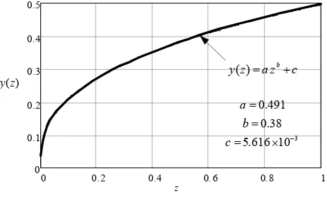
y z az c (18) where _{a0.491;b0.38;c5.616 10} 3 (Figure 2).

Now, applying Equation (13)-(17) we found that P = 14.4 > 14.1. This is sufficient to show that class K1 can give better solutions than class K0. We note that several theoretical and numerical considerations about screw-driver shapes can be found in [14] and the references given there, although applied to the Newton problem of optimal aerodynamic bodies.

4. Formulation of the Optimum Design

Our task is not only to show that class K1 can give better solutions than class K0 as we have seen in the previous section, but also to find the generatrix y(z) for which the corresponding impactor shape belonging to K1 maxi-mizes DOP:

0

( ) max with (0) (free)and (1) (fixed)

y

DOP DOP y

y y y 

 

  (19)

We shall show in the following part of the paper one possible strategy of solution.

5. Psoa Algorithm

To solve this problem we will use the method PSOA (Particle Swarm Optimization Algorithm), a recent heu-ristic suitable for finding global optima solutions. PSOA was introduced about one decade ago [15,16], inspired by the behaviour of school of fish, flocks of birds or swarm of bees observed in nature. Like genetic algo-rithms (GA) and ant colony optimization methods (ACO), PSOA is also a stochastic, population-based global search algorithm. In a natural swarm each individual or particle changes position toward better places, to reach food or to escape from predators, exchanging informa-tion with the neighbourhood and without any central control. In the mathematical model at each individual corresponds a particle and at every particle i is asso-ciated a position vector

i

i

x

in a -dimensional space, to which corresponds a certain value of the objective function

n

( )

i

f x

that represents the quality of

x

_i; of course

x

_i should be a feasible solution to the problem under study . If some constraints must be considered, the objective function can be modified using the penalty technique. When the algorithm starts, a collection (swarm) of particles is randomly chosen using a uniform probability distribution. Then the vector position of each particle is updated at every iteration adding a displace

m

0 0.2 0.4 0.6 0.8 1

0 0.1 0.2 0.3 0.4 0.5

z ( )

y z ( )

b

y z a z c

3 0.491

0.38 5.616 10

a b

c 

 

[image:4.595.312.548.82.225.2]

 

Figure 2. A solution on class K1.

ment based on the information about the previous swarm positions; the knowledge of the gradient of f is not needed. So the iteration rule is the following

(k 1) ( )k (k 1)

i i i

x



_

x

_

s

 ₍₂₀₎

Where ( )k i

x and (k 1)

i

x  _{= positions of particle i at}

k th and k1-iteration, (k 1)

i

s  _{= displacement of}

particle at i k1-iteration.The formula for (k 1)

i

s  _is

( 1) ( ) ( ) ( )

1 1( ) 2 2(

k k k

i i i i g i )

k

s  ws c r p s c r p s (21)

Formula (21) is the core of the algorithm and contains some fundamental information about the neighbourhood of particle i: w is called inertia and serves to control the influence of the previous displacement on the new one. Recommended values of w range from 0 to 1.4; p_i is the best position found for the particle to iteration k, whereas

i

g

p is the best position inside the swarm up to iteration k; c1 and c2 are two positive constants used to balance the cognitive and social aspect: usually c1= c2 = 2.

r1 and r2 are random parameters in the range [0,1], sam-pled from a uniform distribution. The algorithm stops when a prescribed number of consecutive iterations without improvement in the objective function is reached. From (20) and (21) it is clear that PSOA takes account of the previous random walks of particles. During iterations typically two main problems can arise: the first is the explosion of the swarm: it means that the maximum dis-tance between two particles grows indefinitely and con-sequently an overflow error occurs; the second is the stagnation of the swarm which means that all the parti- cles occupy the same position, leading to a suboptimal-solution. To try to avoid such inconveniences the two following additional rules are included in the algorithm: the first rule is the limitation of the maximum displace-ment: ( )

max

k i

problem dependent; the second one is called craziness: with an assigned probability Pcr (for example 0.005), the

displacement (k 1)

i

s  is not calculated with (21) but com-pletely randomly, with the only condition that its modulus must be ≤smax. The PSOA algorithm preposed has several advantages with respect to classical optimi-zation algorithms: 1) it is able to find the true optimum solution in the entire search space (global optimum); 2) it is easy to implement; 3) it can handle non-differentiable function and no calculation of derivatives is required. The main disadvantage is that it can be quite time- consuming. The PSOA algorithm so far described is only one among many others possible that can be found in the current literature [15,17-19]. For the problem under con-sideration the swarm is formed by m particles and each particle is a generatrix yi(z) to which corresponds an

im-pactor shape of class K1 and a certain value of the objec-tive function f (DOP); each generatrix is approximated by the vector y_iwhere every component of y_i is a value of yi; the z axis has been discretized into n-1

inter-vals so we have n points in which to calculate the gen-eratrix; as a consequence the vector yi belongs to an

n-dimensional space; because we know in advance that the most critical zone of the impactor shape in near z = 0, the n-1 intervals of z axis are not equals, but shorter near z = 0 and longer as we go toward z = 1. In our cal-culations n (which corresponds to the swarm size) has been fixed to 30. In Figure 3 some generatrices of op-timum impactors of class K1 are shown using the fol-lowing common parameters: Model n.3, τ =0.5, ω = 14 for different impactor’s speed W = 1.0, 2.0, 3.0, 3.5.

In Table 2 the comparison of DOP of impactors of class K1 illustrated in Figure 3, and the corresponding impactors of class K0 (surfaces of revolution) with the same problem parameters model n.3, τ =0.5, ω = 14, is shown for W = 1.0, 2.0, 3.0, 3.5.

Table 2 shows clearly that the classical and intuitive search space of axisymmetric high speed impactors does not guarantee the best solution (i.e. the maximum DOP). In fact in the cases studied show that an impactor shape belonging to a more general class K1 (non-axisymmetric shape called “screwdriver shape”), can give better results.

6. Concluding Remarks

Starting from the mechanical model proposed by For-restal et al. and using formulas obtained by Ben-Dor et al. for finding the best impactor shape in the class K0 of ax- isymmetric bodies, we presented a different shape of impactors in the new class K1 which is different from the standard axisymmetric shape, and show that bodies be-longing to class K1 can give better results compared to corresponding K0 bodies. We also finalized a code based

z

0 0.2 0.4 0.6 0.8 1.0

0.1 0.2 0.3 0.4 0.5

model:3 0.5

14

 

 

Common Parameters: curve 1

W=1.0

curve 2 W=2.0 curve 4

W=3.5

[image:5.595.311.533.81.224.2]

curve 3 W=3.0

Figure 3. Some generatrices of optimum impactors.

Table 2. Comparison of DOP of impactors.

DOP of impactors of class class K1 with the following common

parameters: modeln.3,  = 0.5,  = 14

Corresponding DOP of impactors of class K0 using

the same parameters: modeln.3,  = 0.5,  = 14 Impaactor’s

speed

DOP of impactor of class K1

Impactor’s speed

DOP of impactor of

class K0

W = 1.0 (curve 1 on

figure.3)

2.0 2.0W = 1.0

W = 2.0 (curve 2 on

figure.3)

6.0 5.8W = 2.0

W = 3.0 (curve 3 on

figure.3)

11.6 11.2W = 3.0

W = 3.5 (curve 4 on

figure.3) 14.7 14.1W = 3.5

on PSOA heuristic algorithm to find the best generatrix in class K0 once some problem parameters are fixed. Some results are also given in a tabular form. We must emphasize that the class K1 is not the most general class of impactors we can imagine so the problem of the best impactor remains open.

7. References

[1] G. Ben-Dor, A. Dubinsky and T. Elperin, “Numerical Solutions for Shape Optimization of an Impactor Pene-trating into a Semi-infinite Target,” Computers and Structures, Vol. 81, No. 1, 2003, pp. 9-14.

[2] G. Ben-Dor, A. Dubinsky, T. Elperin, “Shape Optimiza-tion of an Impactor Penetrating into a Concrete or a Limestone Target,” International Journal of Solids and Structures, Vol. 40, No. 17, 2003, pp. 4487-4500. [3] G. Ben-Dor, A. Dubinsky and T. Elperin, “Modeling of

High-speed Penetration into Concrete Shields and Shape Op-timization of Impactors,” Mechanics Based Design of Struc-tures and Machines, Vol. 34, No. 2, 2006, pp. 139-156. [4] N. V. Banichuk, V. M. Petrov and F. L. Chernousko,

[image:5.595.308.537.266.448.2]

Prob-lems Involving Non-additive Functionals,” USSR Com-putational Mathematics and Mathematical Physics, Vol. 9, No. 3, 1969, pp. 66-76.

[5] M. J. Forrestal and D. Y. Tzou, “A Spherical Cav-ity-expansion Penetration Model for Concrete Targets,”

International Journal of Solids and Structures, Vol. 34, No. 31-32, 1997, pp. 4127-4146.

[6] M. J. Forrestal, B. S. Altman, J. D. Cargile and S. J. Hanchak, “An Empirical Equation for Penetration Depth of Ogive-nose Projectiles into Concrete Targets,” Inter-national Journal of Impact Engineering, Vol. 15, No. 4, 1994, pp. 396-405.

[7] M. J. Forrestal, D. J. Frew, S. J. Hanchak and S. Brar, “Penetration of Grout and Concrete Targets with Ogive- nose Steel Projectiles,” International Journal of Impact Engineering, Vol. 18, No. 5, 1996, pp. 465-476.

[8] G. Ben-Dor, A. Dubinsky and T. Elperin, “Applied High- speed Plate Penetration Dynamics,” Springer, Berlin, 2006.

[9] A. I. Bunimovich and G. E. Yakunina, “On the Shape of Minimum-resistance Solids of Revolution Moving in Plastically Compressible and Elastic-Plastic Media,”Jour- nal of Applied Mathematics and Mechanics, Vol. 51, No. 2, 1987, pp. 386-392.

[10] N. A. Ostapenko and G. E. Yakunina, “The Shape of Slender Three Dimensional Bodies with Maximum Depth of Penetration into Dense Media,” Journal of Applied Mathematics and Mechanics, Vol. 63, 1999, pp. 953-967. [11] G. E. Yakunina, “On Body Shapes Providing Maximum

Penetration Depth in Dense Media,” Doklady Physics,

Vol. 46, No. 2, 2001, pp. 140-143.

[12] G. E. Yakunina, “On the Optimal Shapes of Bodies Moving in Dense Media,” Doklady Physics, Vol. 50, No. 12, 2005, pp. 650-654.

[13] N. V. Banichuk and S. Y. Ivanova, “Shape Optimization of Rigid 3-D High-speed Impactor Penetrating into Con-crete Shields,” Mechanics Based Design of Structures and Machines, Vol. 36, 2008, pp. 249-259.

[14] D. Bucur and G. Buttazzo, “Variational Methods in Shape Optimization Problems,” Birkhauser, Boston, 2005. [15] R. C. Eberhart and J. Kennedy, “A New Optimizer Using

Particle Swarm Theory,” Proceedings of the 6th Interna-tional Symposium on Micromachine and Human Science, Nagoya, 1995, pp. 39-43.

[16] J. Kennedy and R. C. Eberhart, “Particle Swarm Optimiza-tion,” Proceedings of the IEEE International Joint Con-ference on Neural Networks, Perth, 1995, pp. 1942-1948. [17] M. Clerc, “Particle swarm optimization,” ISTE, London,

2006.

[18] M. M. Ali and P. Kaelo, “Improved particle swarm algo-rithms for global optimization,” Applied Mathematicsand Computation, Vol. 196, 2008, pp. 578-593.

[19] P. C. Fourie and A. A. Groenwold, “The Particle Swarm Optimization Algorithm in Size and Shape Optimiza-tion,”Structural and Multidisciplinary Optimization, Vol. 23, No. 4, 2002, pp. 259-267.