A Note on “Limit Distributions of Self Normalized Sums” Using Cauchy Generated Samples

(1)

ISSN Print: 2152-7385

DOI: 10.4236/am.2019.1011062 Oct. 25, 2019 863 Applied Mathematics

A Note on “Limit Distributions of

Self-Normalized Sums” Using

Cauchy-Generated Samples

Jan Vrbik

Department of Mathematics and Statistics, Brock University, St. Catharines, Canada

Abstract

In this case study, we would like to illustrate the utility of characteristic func-tions, using an example of a sample statistic defined for samples from Cauchy distribution. The derivation of the corresponding asymptotic probability den-sity function is based on [1], elaborating and expanding the individual steps of their presentation, and including a small extension; our reason for such a plagiarism is to make the technique, its mathematical tools and ingenious ar-guments available to the widest possible audience.

Keywords

Self-Normalized Sum, Cauchy Distribution, Characteristic Functions, Fourier Transform, Padé Approximation

1. Introduction

The problem of finding the distribution of self-normalized sum of a Cauchy- generated sample has been considered since at least 1969 (see, for example, [2]), but solved (by proposing a concrete numerical algorithm) only in 1973 by [1], our key reference. After that, the research has been focused mainly on proving general statements concerning self-normalized sums, without dealing with spe-cific distributions such as Cauchy—see, for example, [3].

In this article, we demonstrate how characteristicfunctions (CHF) are used in Statistics to find a distribution of a specific samplestatistic (a function of indi-vidual observations). We do this by using a single comprehensive example, namely finding the n→ ∞ limit of the probability density function (PDF) of

1 2 1 n

i i

n i i

X X =

=

∑

(1) How to cite this paper: Vrbik, J. (2019) A

Note on “Limit Distributions of Self-Nor- malized Sums” Using Cauchy-Generated Samples. Applied Mathematics, 10, 863-875.

https://doi.org/10.4236/am.2019.1011062 Received: August 20, 2019

Accepted: October 22, 2019 Published: October 25, 2019

http://creativecommons.org/licenses/by/4.0/

(2)

DOI: 10.4236/am.2019.1011062 864 Applied Mathematics where X X1, , ,2 Xn is a random independent sample (RIS) of size n from a

Cauchy distribution with zero median. This goal has already been achieved (in a more general setting) by [1]; our main (rather pedagogical) reason for extending their presentation is to make it accessible to graduate and advance undergra-duate students.

First we recall that the CHF of a random variable X is defined by

( )

isX _cos

( ) ( )

_d _{i sin}

( ) ( )

_d

x s e sx f x x sx f x x

ϕ = =

_∫

_−∞∞ ⋅ +

_∫

_−∞∞ ⋅ (2) where f x

( )

stands for the X’s PDF,  for the corresponding expected value, and i is the purely imaginary unit; note that the real part of

ϕ

x

( )

s is always an even (an alternate name is symmetric) function of s, while the purely imaginary part is odd. Also note that when f x

( )

is even, the corresponding CHF must be

real (its purely imaginary part becomes zero because the integrand is odd). Similarly

( )

(

i i

)

i i

( )

- plane

, esX tY esx ty , d d

xy

x y

s t f x y x y

ϕ ₌ + ₌ + _⋅

∫∫

 (3)

(where f x y

( )

, is the joint PDF of X and Y) defines the joint CHF of two (not necessarily independent) random variables X and Y; when they are independent, we have

( )

,

( ) ( )

xy s t x s y t

ϕ

=

ϕ

⋅

ϕ

₍₄₎ (product of the individual CHFs). This implies that (when independent), the CHF of X Y+ _{is given by}

ϕ

_x

( ) ( )

s ⋅

ϕ

_y s _{, further implying that the CHF of a}

samplemean of n independent Xi is given by n x _ns

ϕ  _{ }

  (5)

When two random variables are combined into one (e.g. defining U X Y

= _),

the CHF of U is given by

( )

i i

( )

- plane

e e , d d

x

X _s

s _y

Y U

x y

s f x y x y

ϕ

= __ ⋅ __= ⋅ ⋅

 

∫∫

 (6)

Under very general conditions, knowing a generating function enables us to reverse the process and find the corresponding PDF thus:

( )

1 _e i

( )

_d

2 sx x

f x = _−∞∞ − ϕ s s

π

∫

(7)

To learn more about the mathematical details of transforming PDF into CHF and back the reader may like to consult [4].

2. Joint CHF and Its Limit

Assume a RIS of size n from a Cauchy distribution with the following PDF

( )

(

2

)

1 1

g x

x

=

(3)

DOI: 10.4236/am.2019.1011062 865 Applied Mathematics The joint CHF of X and _X2_{(seen as}_distinct_{random variables) is then given} by

(

2

)

( )

exp ixs x t g x xi d

∞

−∞ +

∫

(9)

This implies that the joint CHF of

def ni₁ i n

X U

n =

=

∑

₍₁₀₎

and of

2 def

2 1

2

n i i n

X V

n =

=

∑

₍₁₁₎

is (replace s by s

n and t by 2 t

n in (9), and raise the result to the power of n)

( )

2

2 ,

i i i

, 1 exp 1 d

n n

n

U V

xs x t xs

s t g x x

n n n

ϕ =_ + _−∞∞ _ _ + _− − _ _

   

   



∫

 (12)

where adding and subtracting 1 facilitates taking the n→ ∞ limit; similarly, subtracting ixs

n (which does not change the value of the integral since it inte-grates, in the principal-value sense, to 0) helps to make subsequent integrals converge. Note that principal value of an integral implies replacing

_∫

_−∞∞dx by

lim_R_{→∞ −}

_∫

R_Rdx; this is tacitly assumed from now on. Replacing x by ny makes the previous expression into

(

)

( )

{

₁ ∞ _{exp i}_{ys y t}_i 2 _{1 i}_{ys g ny n y}_d

}

n

−∞ 

+

_∫

_ + − − _ ₍₁₃₎

whose n→ ∞ limit is

(

2

)

2

d exp exp iys y ti 1 iys y

y ∞

−∞

 _ ₊ _{− −} _ 

 _ _{ π} 



∫

 (14)

since

( )

2 2

1

g ny n u

→ _and 1 exp

( )

n

A _A

n

 ₊  _→

 

  . The last displayed expression is

thus the characteristic function of U and _V2_{(our notation for the} correspond-ing limits of Un and Vn2).

Note that only the tail behaviour of (8) was relevant in the end.

3. Finding CHF of (1)

Replacing t by _i_{s w}2 _(with_w_positive_{) results in}

(

)

(

)

( )

2 2

,

2 2

2

,i

d

exp exp i 1 i exp

U V s s w

y

ys s wy ys s w

y

ϕ

ψ

∞

−∞

 _ _ 

= _ _ − − − _{ π} _= _ _



∫



(15)

(4)

DOI: 10.4236/am.2019.1011062 866 Applied Mathematics

( )

def

(

₂

)

2

d exp i 1 i

2 1 ₂ _exp 1

4 2

z

w z wz z

z w Q w w ψ ∞ −∞  = _ − − −  π     = − _ _− _− _

π   π  

∫

(16)

with

( )

def 2

0exp ₂ d z

Q τ = τ _− _ z

 

∫

(17)

Note that the value of

ψ

( )

w _{is thus always}_negative_{(this remains true for} the real part of

ψ

( )

w after we make w complex; this becomes consequential later on). Proof.

( )

(

)

(

)

(

)

2 2

i 2 ₂

i 2

2

1 _{exp i} _d

1_exp 1 _exp i _d

4 2

1_exp 1 _exp _d

4

1_exp 1 _exp _d

4 1 exp 4 w w

w z wz z

w z z

w w wt t w wt t w w w

ψ _−∞∞

∞ −∞ ∞− −∞− ∞ −∞ ′ = − − π       = − _− _ _− _ − _ _ π   _   _

 

= − _− _ − π  

 

= − _− _ − π  

₋      = − π

∫

since moving the path of the t integration does not change the integral’s value (there are no singularities between the two paths) and the integrand tends to 0 sufficiently fast within the same strip when w tends to plus or minus infinity.

Therefore,

ψ

( )

w is given by

2

1 _exp

exp

2

4 d d

z z

w w C z C

z w   ₋  ₋         − + = + π π

∫

(18)

2

exp

2 _{2 exp} _d

z

z z _z

z z   −   _ _   = − − _− _

π π

∫

_ _ (19)

1 2 1

2 exp 4 2 w _Q w w     = − _− _− _ _

π   π   (20)

using the 1₂ 2

w z

= substitution. Note that C=0, since

( )

2

Q ∞ = π_and

( )

0 1 exp i

( )

z₂ 1 izdz 1

z

ψ = _−∞∞ − − = −

π

∫

(21)

(5)

DOI: 10.4236/am.2019.1011062 867 Applied Mathematics since the integrand has no singularities between the two paths), and then eva-luating

( )

i

2 2 0 2

exp i 1 i i e

lim d lim d 0 lim e d

e t

t it

R R R

z _z z _z R _t

z z R

π

→∞ →∞ →∞

+ −

− = + ⋅ = −π

∫



∫



∫

(22)

The first integral is equal to 0 due to Jordan’s lemma. In the second integral, we have traded the clockwise half circle for counter-clockwise (by changing the integrand’s sign).

Evaluating (15) at two distinct values of w (let us denote them w and w0),

di-viding the difference by s, and integrating over s from 0 to infinity yields

( )

(

)

(

)

( )

2 2 2 2

0 0 0

0 0

exp exp

exp i , d d d

exp exp

d

s v w s v w

su f u v u v s

s

s w s w

s s ψ ψ ∞ ∞ ∞ −∞ ∞ − − − ⋅   −       =

∫ ∫ ∫

∫

(23)

where f u v

( )

, is the joint PDF of U and V; note that its support is the whole upper half of the u-v plane.

Replacing s by t

v (note that v cancels out from

ds dt

s = t ) changes the left hand side of (23) to

(

2

)

(

2

)

_{( )}

0 0 0

exp exp

exp itu t w t w f u v u v t, d d d

v t ∞ ∞ ∞ −∞ − − −   _⋅    

∫ ∫ ∫

(24)

( )

(

2

)

(

2 0

)

0

exp exp

d

t w t w

t t

t

ϕ

∞ − − −

=

_∫

⋅ (25)

where

ϕ

( )

t is the characteristic function of U

V , the variable whose distribu-tion we seek; the last expression is then equal to the right-hand side of (23).

4. Converting to PDF

Differentiating the resulting equation, i.e. (25) = (23), with respect to w then yields (after a sign reversal)

( )

(

2

)

( )

_{( )}

( )

0 exp d 0 exp d

w

t t t w t w s w s

w

ψ

ϕ

ψ

∞ ∞ ′

′

⋅ − = − _ _ =

∫

(26)

(to the last integrand,

ψ

( )

w is just a negative constant). Finally, multiplying both sides of the previous equation by

2 exp 4 y w w      

π π (27)

and integrating over w from 0 to i⋅ ∞_{(a notation which implies following the}

positive imaginary axis) results in

( )

(

)

_{( )}

( )

2 i 3 2 0 0 exp 4

1 _{exp i d} 1 _d

y

w w

t ty t w

w w ψ ϕ ψ ∞ ⋅∞     _′   ⋅ − = ⋅

(6)

DOI: 10.4236/am.2019.1011062 868 Applied Mathematics where w denotes the corresponding principal value, and (16) is now ex-tended to complex arguments.

Proof. Following [5], we write 2 2 i ₂ 2 0 0 2 i 0 exp

4 _d 2 i _exp i 1 _d

2

2 i i 1

e exp d

2 ty

y _{t w}

w _w y ty _z _z

t z

w

y _{ty z} _z

t z ⋅∞ ∞ ∞ −   −   _ _     ₌ ₋ ₊  _ _    _ _  = _− _ − _ _    

∫

(29) after introducing 2 i 2 z y w t

= ₍₃₀₎

A further z 1 z

substitution makes it into 2 i

2 0

2 i i 1 d

e exp

2

ty y ty _z z

t z z

∞

− _₋  ₋  _

 

 _ _ 

 

∫

(31)

Adding (29) and (31), which are identical in terms of their value, and dividing by 2 yields

2 i

2 0

i i 1 1

e exp 1 d

2 2

ty y ty z _z

t z z

∞

− _₋  ₋  _ ₊ 

   

 _ _{ } _

 

∫

(32)

Finally, introducing q z 1 z

  =_ − _

  results in

i i i 2 i

e exp d e

2 2

ty y ty q q ty

t t ∞ − − −∞ π ₋  ₌ _⋅    

∫

(33)

assuming that, to evaluate the last integral, we first replace t by t−iε (to make it converge), and then take the ε→0 limit of the answer (Cauchy-type inte-gration).

It is well known that the realpart of the left hand side (and, therefore, of the right-hand side) of (28) yields the desired (clearly symmetric) PDF of U_V , say

( )

f y , due to

ϕ

( )

t being real (and thus automatically symmetric as well). This then yields

( )

_{( )}

( )

2

i 3 2 0

2

i

3 2 ₀ 3 2

exp 4

1 Re d

exp 4

2_Re d

1 1 1

2 ₁ _exp

4

2 2

y

w w

f y w

w w y w w w _Q w w w ψ ψ ⋅∞ ⋅∞     _′   = ⋅ π       = ⋅

π ₊    

   

   

∫

(34)

(7)

DOI: 10.4236/am.2019.1011062 869 Applied Mathematics In an attempt to break this impasse, we introduce the following substitution

2

1 2

w

τ

= (35)

getting

( )

2 2

exp i 4

3 2 0 2

exp d

2 2 Re

1 exp

2

y f y

Q

τ _τ

τ

τ τ

− π ⋅∞

      =

π  

+ _ _  

∫

(36)

where τ now follows the complex ray at −45˚.

Unfortunately, even after this substitution, special measures are still needed to facilitate accurate numerical integration of the integral. For one, it becomes ne-cessary to separately deal with the _y2_<₁_and _y2_>₁_regions.

5. Case of

y

2

_{< 1}

When _y2_<₁_{, it is legitimate to rotate the ray of the last integration to the} posi-tive real axis, since there are no singularities of the integrand between the old and the new path, and the function decreases sufficiently fast towards infinity in that segment. We then get

( )

2 2

3

2 0

2 exp d

2

1 exp

2

y f y

Q

τ _τ

τ

τ τ

∞

    π _ _ =

  + _ _  

∫

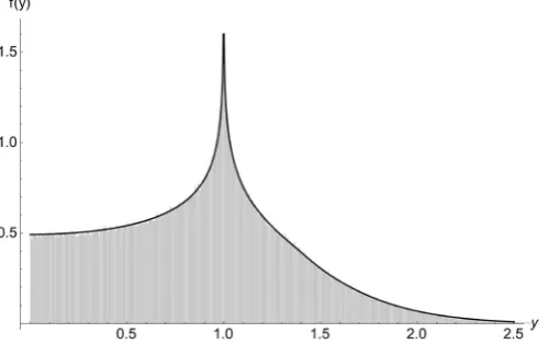
(37)

where τ is real, and the integrand is “well behaved” (no oscillations). Results of numerical evaluation are displayed in Figure 1 (we are showing only the

0

y> portion of the graph; visualize a mirror image of this curve when

1 y 0

− < < ).

[image:7.595.228.536.91.201.2] [image:7.595.251.501.533.690.2]

To investigate the nature of this singularity we notice that, for large τ , the integrand of (37) tends to

(8)

(

)

2 2

2

1 2 exp

2

y

τ τ

 − 

 

⋅ −

 

π _ _ (38)

since Q

( )

τ

_τ_→∞→ π2_{. Integrating the last function over}τ from 0 to in-finity yields

2

1 _0,1 2

y

 − 

⋅Γ 

π _ _ (39)

where the second factor is a special case of the incomplete gamma function de-fined by

( )

def

( )

1

0, ln

!

k

z

z z

k k

γ

∞

=

−

Γ = − − −

⋅

∑

(40)

and γ is Euler’s gamma. This indicates that, by adding _{ln 1}

(

₋_y2

)

_π−2 to

( )

f y makes the resulting function finite (and thus amendable to a simple, Padé-type approximation, constructed later on).

6. Case of

y

2

_{> 1}

The situation becomes somehow more difficult when _y2_>₁_{. Now, we can} ro-tate the −45˚ ray of the (36) integration to −90˚ (the negative imaginary axis), since the integrand decreases sufficiently fast towards infinity in this range of directions. The new path contributes 0 to the real part of (36), since the inte-grand (along the −90˚ ray) is real and dτ is purely imaginary. But moving from −45˚ to −90˚ we have crossed infinitely many singularities located between the two rays; these can be found numerically (a rather tedious procedure) by solving

( )

2

1 exp 0

2 Q

τ

τ   τ

+ _ _ =

  (41)

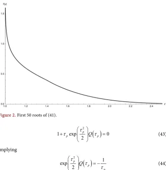
The location of the first 50 of these (they are all simple poles, slowly converg-ing to the Imτ = −Reτ line) are shown in Figure 2.

We can then evaluate (36) using Cauchy integral theorem; note that, at each of these poles (say at τp), the τ derivative of

( )

2

1 exp 2 Q

τ

τ   τ

+ _ _

  equals to

1

p

τ

− _{, since}

( )

2

2 2 2 2

2

d 1 exp 2 d

exp exp exp exp

2 2 2 2

p

p p p p

Q

Q Q

τ τ

τ

τ τ

τ

τ τ τ τ

=

   

+

   

 _ _ 

 

       

= _ _ + _ _ + _ _ _− _

       

(42)

(9)

[image:9.595.210.537.68.404.2]

DOI: 10.4236/am.2019.1011062 871 Applied Mathematics Figure 2. First 50 roots of (41).

( )

2

1 exp 0

2

p

p Q p

τ

 

τ

+ _ _ =

  (43)

implying

( )

2

1 exp

2

p p

p

Q

τ

 

= −

 

  (44)

This means that each pole (with the exception of the first one—see the next paragraph), contributes

2 2

3

2 Re 2 exp

2 p p

y

i τ τ

   π ⋅

 _ _

π __ _ ___ (45)

to (36).

The pole on the imaginary axis needs to be avoided by an infinitesimal half

circle, which means that it contributes only one half of the above amount, namely

2 2

2 _1.30693exp 1.30693 2

y

 

⋅ _− _

π _ _ (46)

The last function yields the asymptotic behaviour of f y

( )

as _y2_{→ ∞}_{, and} provides an excellent approximation (its maximum absolute error is about

6

2 10_× − _{) to this PDF when} _y _>_1.8_{. Unfortunately, to build a numerical} solu-tion for the full range of _y2_>₁_{values by adding contributions of sufficiently} many of these poles (as done by [1]) is rather tedious, as finding hundreds of these poles (needed to reach a good accuracy, especially when _y2_{approaches 1)} is a non-trivial task, and the resulting convergence is quite slow.

(10)

DOI: 10.4236/am.2019.1011062 872 Applied Mathematics 2 2

2 2

2

2 Im exp 2

y

τ

  

− _π _  _

 

  (47)

where τ = −2 1.84906 3.45208i− , to (46) results in an equally accurate approxi-mation (its error is less than _{2 10}_× −6_{) in the} _y _>_1.7_{tails of} _{f y}

( )

_.

7. Alternate Solution

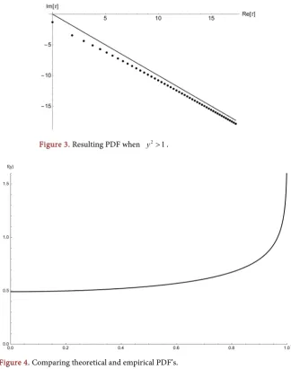
We are now going to backtrack and deal directly with (36). Even though its inte-grand is still highly oscillatory (with a frequency which increases as

i 4

e

τ_{→ ∞ ⋅} − ⋅π _{), we can mitigate the problem by dividing the range of integration} into two segments: first we integrate from 0 to 1 i− (which does not pose any numerical difficulty), thus getting what we will call the first component of (36), then from 1 i− _{to infinity (along the −45˚ ray), getting the}_second_component.

To carry out the latter integration, we first note that, for large τ , Q

( )

τ

can be expanded in the following manner

( )

exp 2 1 1₃ 3 5 3₅ ₇

2 2

Q τ τ

τ τ τ τ

 

π₋ ₋ _⋅ ₋ ₊ ₋ ⋅ ₊ 

  _ _

 

 (48)

Substituting this into the integrand of (36) and further expanding in powers of 1

τ (up to and including the 6th power) while keeping the two exponential terms

fixed (i.e. not expanding in τ ) yields

(

)

2 2

4 6

2exp 6exp ₁

2 2

2 1 _exp

2

y

τ τ

τ

τ τ τ

    

− −

     _ ₋ _    

 _{⋅ −} ₊ _⋅ _₋ _

 _π _π _π  _ _

 

 

 

(49)

which can be τ -integrated, from 1 i− _to ∞ −

( )

1 i _,_analytically_{; then we}

nu-merically integrate (over the same line segment) the difference between the inte-grands of (36) and (49)—since the resulting integrand now approaches zero (as

τ _{increases) very quickly, the integration range becomes effectively finite (}1 i−

to 6 6i− _{already achieves very high accuracy), thus eliminating any}

trouble-some oscillation. Adding the real part of the last two answers (and multiplying by ₂_π−3 _{) then provides the second component of} _{f y}

( )

_.

This technique yields the graph of Figure 3 (drawn for y>1; visualize a mirror image of this curve when y< −1):

8. Monte-Carlo Verification

One can always get a good idea about a distribution of any sample statistic (however complicated and inaccessible to analytic treatment) by actually gene-rating a random sample with the required properties by a computer, and using it to compute the desired statistic’s value; this is then repeated as many times as possible, displaying the results in a histogram.

(11)

DOI: 10.4236/am.2019.1011062 873 Applied Mathematics its random values. Plotting the resulting histogram, together with the theoretical asymptotic PDF of the last three sections, yields Figure 4; visual comparison clearly indicates a good agreement between the two answers. The tiny discre-pancy still discernible (mainly in the 0< <y 1_{range) is due to the fact that}

100

n= is not large enough to have reached the n→ ∞ limit yet (trying to make the sample size substantially higher would run up against our computer’s capacity).

Note that, to be more economical, we have folded the negative and positive parts of the distribution into a single graph, effectively plotting the PDF of the

absolutevalue of (1).

9. Accurate Approximation

First we have to remember the we already have an excellent approximation to

( )

f y in the y >1.7_{region, given by the sum of (46) and (47); now we have} to find a similarly accurate way of dealing with y ≤1.7.

[image:11.595.208.533.311.723.2]

Figure 3. Resulting PDF when _y2_>₁_.

(12)

DOI: 10.4236/am.2019.1011062 874 Applied Mathematics We already know that, by adding

2

ln 1−y

π (50)

to f y

( )

removes the corresponding singularity when _y2_≤₁_{; we can easily} verify that the same is true when _y2_>₁_{, since one of the terms in the analytic} result of the (49) integration (once we take its real part and multiply by ₂_π−3

) equals to

2

1 _Re _0,i 1 2

y

 − 

⋅ Γ_ ⋅ _

π _ _ (51)

where

(

)

( )

_{( )}

2

1

Re 0,i ln

2 2 !

k k

k

z

z z

k k

γ

∞

=

−

Γ ⋅ = − − −

⋅

∑

(52)

whose singular part is given by (50). This proves that

( )

2 2

ln 1 y

f y + −

π (53)

is singularity-free for all values of y; unfortunately, that still does not make it sufficiently “smooth”, as the next paragraph indicates.

There is yet another subtle issue causing great difficulty when trying to build an approximate formula for (53): the function has a small (hardly noticeable) kink (a discontinuous second derivative) at _y2₌₂_{; this is not an artifact of the} new technique—the same (rather surprising) phenomenon can be confirmed by the old technique of adding residues. Luckily, we can identify yet another term of the (49) contribution responsible for this discontinuity, and remove it by fur-ther subtracting the offending term from (53), thus getting

( )

(

) (

)

3 2

2 2

2

2 2

2Re 2 3 11

ln 1

. 15

y y

y

f y + − − − −

π π (54)

This function is (finally!) sufficiently (even though not perfectly—tiny issues remain with higher derivatives at _y2₌_2,_y2 ₌₃_{etc.) smooth to fit it (in the}

1.7

y < _{range) by a ratio of two polynomials (by minimizing the total error}

squared). This results in the following approximation

2 4 6 10

2 4 6 10 14

0.666457 0.82876 0.401154 0.0800733 0.00203206 _. 1 0.572265 0.0327094 0.0207377 0.00042241 0.000261666

y y y y

y y y y y

− + − +

− + + + + (55)

Its absolute error never exceeds _{6 10}_× −6_{, which is more than sufficient for} any practical application. The form of this expression and the individual powers of y have been chosen somehow arbitrarily; we do not claim that our choices are optimal.

(13)

10. Conclusion

The aim of this article was to demonstrate that finding the distribution of a rela-tively simple sample statistic requires a skillful use of characteristic functions and a whole gamut of sophisticated mathematical techniques, including real and complex analysis, Fourier transform, and curve fitting. We hope that students of Statistics can benefit from the ingenuity of the authors of the original derivation of this distribution as presented in [1], and from some extra details included in this article; the latter includes a different numerical approach to building the re-sulting PDF, expressing it in the form of an accurate Padė-type approximation (discovering an interesting discontinuity in the process), and verifying the an-swer by Monte Carlo simulation.

Conflicts of Interest

The author declares no conflicts of interest regarding the publication of this pa-per.

References

[1] Logan, B.F., Mallows, C.L., Rice, S.O. and Shepp, A.L. (1973) Limit Distributions of Self-Normalized Sums. The Annals of Probability, 1, 788-809.

https://doi.org/10.1214/aop/1176996846

[2] Efron, B. (1969) Student’s t-Test under Symmetry Conditions. Journal of the Amer-ical StatistAmer-ical Association, 64, 1278-1302.

https://doi.org/10.1080/01621459.1969.10501056

[3] Spătaru, A. (2014) Convergence and Precise Asymptotics for Series Involving Self- Normalized Sums. Journal of Theoretical Probability, 29, 267-276.

https://doi.org/10.1007/s10959-014-0560-1

[4] Sneddon, I.N. (2010) Fourier Transforms. Dover Publications.