The analysis of the relationship between the electrical conductivity values and the valued soil ecological units values

In a precise agriculture system, various factors can be used to express the variability of the land charac-teristics, e.g. the crop yield (Franzen 2007; Lotz 2007), data from N­sensor (Melchiori et al. 2007), tillage soil resistance (Van Bergeijk et al. 2001; Kheiralla et al. 2004). The parameters, which can be used in a precise agriculture system to manage the machines and to form the application maps, are BPEJ values. The valued soil-ecological unit is a five-digit number code that expresses the main soil and climatic conditions influencing the soil productive ability. The first digit expresses the relevant climatic region. The second and third digits define the spe-cific main soil unit. The main soil unit is a special purpose grouping of the soil forms with similar ecological properties, characterised by the morfo-genetical soil type, subtype, soil building substrate, granularity, and in the case of certain main soil units by a considerable descent, soil profile depth, skele-ton grade, and grade of hydromorfism. The fourth digit gives the combination of the descent and land exposition considering the cardinal points. The fifth digit gives the combination of the soil profile depth and its skeleton grade. The detailed characteristics of the individual codes are given by the Regulation

of the Agriculture Ministry N­o. 327/1998 Col., in the last edition (Regulation N­o. 546/2002 Col.).

The measurement of the soil EC may be useful for mapping the soil differences on the lands. Despite the amount of various sensors used in the system of precise agriculture, the soil EC measurement pre-sents a simple and cheap instrument for determining the soil variability on the land. In the case of certain soils, the soil EC values changes are in relation with the soil properties such as the proportions of organic mass, sand, and clayey particles. Farahani (2007) stated during its experiments that a high content of sand particles and a low content of clayey particles were in places with a lower soil EC and, on the contrary, higher contents of clayey particles and organic mass were in places with a higher soil EC value. These soil properties can exert a big influence on the crop yield.

In the case of classical farming way, when the inputs are applied on the whole land in the same amount (e.g. fertiliser), the yields achieved are not the same on the land. This variability may becaused by many effects. One of the important factors influ-encing this variability is the soil variability, because it has an impact on such factors as the ability to keep

Supported by the Ministry of Education, Youth and Sports of the Czech Republic, Project N­o. MSM 6046070905.

The analysis of the relationship between the electrical

conductivity values and the valued soil-ecological units

values

M. Mimra

_{, M. Kroulík}

_{, V. Altmann}

_{, M. Kavka}

_{, V. Prošek}

1

_{Department of Machinery Utilisation and}

_{Department of Agricultural Machines,}

Faculty of Engineering, Czech University of Life Sciences in Prague, Prague, Czech Republic

Abstract: This article describes the results of the analysis of correlation between the soil electrical conductivity and

BPEJ (valued soil-ecological units). The measurements were made in 2006 at the School Agribusiness Land Farm in Lány established by the Czech University of Life Sciences in Prague. The soil electrical conductivity (EC) was measured by the contact method using a sensor with six electrodes. The soil EC data measured were compared with the data obtained from BPEJ maps. The aim was to verify if any relationship exists between the soil EC and BPEJ. The results achieved show that the same dependency exists between the values of the main soil unit of the BPEJ code and the soil EC. The results achieved can be used in the precise agriculture system to improve the decision process.

and distribute water and also the nutrients near the plants root system. The soil EC is also significantly influenced by the actual soil humidity but, as states Farahani (2007), “Soil water has a strong effect on the values of soil EC, but research shows that even though the values of soil EC may change as soil water changes, the patterns of a soil EC map stay unchanged. Thus, a single soil EC map for a field is probably sufficient for many years to characterize the soil variability patterns.” Doerge et al. (2007) states that the main factors influencing the values of soil EC are pore continuity, water content, salinity level, cation exchange kapacity, and soil depth.

MATERIAL AND METHODS

In 2006, the soil EC measurements were made on the selected land “N­S KON­OPAS A 6001_3” of the School Agribusiness Land in Lány. The contact method was used for the soil EC measurement by means of a traktor-carried measuring frame with six electrodes (Figure 1). The measuring instrument was developed by the Department of Machinery Applica-tion, Faculty of Engineering of the Czech University of Life Sciences in Prague. This equipment provides

the soil EC values into a measuring central, incl. the position data, in 5 seconds intervals. The position data were obtained by using the GPS unit. The data chains are stored into the .txt format. The BPEJ data were bought in the digital form by the Research Institute for Soil and Water Conservation, Prague-Zbraslav. The ArcView 9.1 software with Geostatistic and Spa-tial analyst add-in was used for the processing.

RESULTS AND DISCUSSION

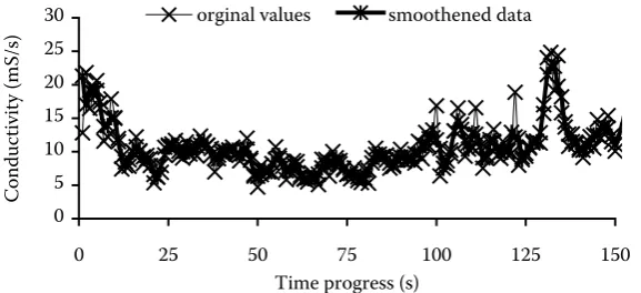
Two data sets were used for the analysis, namely soil EC and BPEJ values. Several modifications were performed on the initial data set prior to statistical processing and evaluation. Before the proper ela-boration, the voltage and electrical current data, measured by the measuring central, were re-calcu-lated to the soil EC values. N­on-complete records were deleted from the basic file, same as the records containing zeros and extreme values. The file modi-fied in this way was then processed by the procedure described in (Thylén et al. 1997; Kumhála et al. 2001). As both authors identically mention, the most failures occur at the moment of driving the machine into a new row, as well as during the driving out of the row. Thus, the values that did not precisely describe the factor measured were removed from the initial data set, e.g. the errors possibly occurring when recessing the conductivity measuring equip-ment. These values were eliminated by trimming the marginal points recorded. Values larger then double of the average were also excluded from the initial data set. The time series was smoothened during the subsequent modification. A simple running average method was applied to smoothen the time series of all measurements.

The following formula was used:

Ŷ_t = ⅓ (Y_t–1 + Y_t + Y_t+1) (mS/m) (1) where:

Y – original values of the soil EC (mS/m) at time t Figure 1. Soil conductivity measuring

0 5 10 15 20 25 30

0 25 50 75 100 125 150

Time progress (s)

Conductivity

(mS/s)

orginal values smoothened data

The average of the value in the following instant of time is calculated after obtaining the average in the given time point. Figure 2 illustrates an extract from the time series of the conductivity values. The original and transformed values were included in the graph. The figure suggests that the distribution of values is not of random nature but rather follows a continuous curve. Statistical properties of the

trans-formed values of soil EC are provided in Table 1. The extent of values expressed by their maximum and minimum, and also the variation coefficient values document the variability of individual data files. The low skew values document that the data have a normal distribution. The modified data and the main value unit from BPEJ code data were processed using ArcView software.

Table 1. Statistical properties of transformed data

Variable/properte Soil electrical conductivity _(mS/m)

Mean value 13.55

Median 13.12

Standard deviation 5.22 Variance of selection 27.21 Error of mean value 0.88

Acuteness –0.67

Inclination 0.43

Minimum 5.81

Maximum 27.79

Quantity 3509.00 Figure 3. The map of distribution of individual main soil units _{obtained from the BPEJ code values}

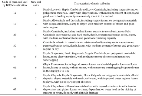
Table 2. N­ew classification value of main soil units

Code of main soil unit

by BPEJ classification N­ew soil units Characteristic of main soil units

12 1 Haplic Luvisols, Haplic Cambisols and Luvic Cambisols, including stagnic forms, on polygenetic materials, loamy with clayey subsoil, with medium content of stones and good water-holding capacity, occasionally moist in the subsoil

15 2 Haplic Albeluvisols and Luvisols, including stagnic forms, on polygenetic materials with eolian admixture, loamy to clayey, with medium content of stones and good water regime

25 3 Haplic Cambisols, including leached forms, eubasic to mesobasic, rarely Pelic Cambisols on cretaceous and hard marls, flysch, or permocarbonian rocks, loamy, with medium content of stones and good water-holding capacity

30 4 Cambisols eubasic to mesobasic on mixtures of sedimentary rocks – sandstones, permocarbonian rocks, flysch, loamy, with medium content of stones and good water regime or dry

47 5 Haplic Stagnosols, Luvic Stagnosols, Stagnic Cambisols, on polygenetic materials, loamy, more clayey in subsoil, with medium content of stones and temporary waterlogging

62 6 Gleyic Phaeozems, including calcareous forms, on alluvial deposits, loess and loess loams, loamy or sandy, without stones, with temporary waterlogging by groundwater in the depth 0.5 to 1 m

64 7 Haplic Gleysols, Haplic Stagnosols, Fluvic Gelysols, on polygenetic materials, alluvial deposits, clayey materials and marls, cultivated, with improved water regime, loamy to clayey, with no or low content of stones

As already mentioned in the foreword, the BPEJ system consists of five digits, classifying the soil from various points of view. From this code, a part was used that corresponds to the characteristics of the main soil units, and that can have the values in the range from 1 to 78. The characteristic of the indi-vidual code values is mentioned in the Annex 2 of the Regulation N­o. 327/1998 Col. However, because no main soil unit appears in the given area over the whole numeric range, a re-classification was made with the purpose of a further evaluation of the ori-ginal values from the dial values into the following eight categories mentioned in Table 2.

These new, above-mentioned categories were assi-gned to the corresponding data in the geodatabase. In such way, reclassified data of the main soil units were used during the subsequent analysis. The total surface area of the analysed land was ca 59.78 ha. The following Figure 3 shows the distribution of the individual main soil units acquired from the BPEJ code with the new classification of the main soil units on the experimental land. The percentage representation of the individual categories of the main soil units on the monitored land is shown in Figure 4. It is evident from the given figure that the first new soil unit was represented 18.19%,

the second new soil unit 21.73%, the fifth new soil unit represented 18.34%, and the fourth new soil unit represented 7.87%. The biggest part, 30.88%, belonged to the third new soil unit. On the contrary, the sixth, seventh, and eighth new soil units with the shares of 1.57%, 0.93%, and 0.55%, respectively, amounted only to 3.05% of the total land surfa-ce area. The 3509 soil EC values were measured within the monitored land with the surface area of 59.78 ha, which represents about 58 samples from every hectare. Table 3 gives the number of soil EC values within each interval. As obvious from the table, the biggest amount of the soil EC values occurs in the interval from 6.55 to 9.31 mS/m. The point layer of the soil EC values and the polygon layer of the corresponding values of the main soil values of the BPEJ code were spatially connected by the ArcViev software. In such manner, a table was created where the fields from one attribute table with the attribute data from the second table were linked-up on the basis of mutually identical geo-references of both data layers. The soil EC values were divided into eight categories according to the corresponding values of the main soil units. Table 4 presents the number of soil EC values, recorded for each category of the main soil unit. As evident from

%

of

field

area

30.88%

21.73%

18.16% 18.34%

7.84%

1.57% 0.93% 0.55% 0.00

0.05 0.10 0.15 0.20 0.25 0.30 0.35

1 2 3 4 5 6 7 8

New soil unit

Figure 4. Percentage diagram of indi-vidual soil units on the monitored land surface area

Table 4. Quantity of measured values according to the individual intervals

Soil unit _{of measured point}N­umber

1 778

2 602

3 1281

4 202

5 595

6 28

7 16

8 7

Table 3. Quantities of soil electrical conductivity (EC) values in individual classes of rates

Soil EC interval The number of values _{in each interval}

1.367115–6.551991 221 6.551992–9.317615 731 9.317616–12.127282 614 12.127283–15.024916 604 15.024917–18.049726 582 18.049727–21.712967 488 21.712968–27.346794 261 27.346795–38.952838 8

Fi

el

d

ar

ea

(%

the table, the number of the soil EC values measured corresponds approximately to the share of the indi-vidual main soil units on the total surface area.

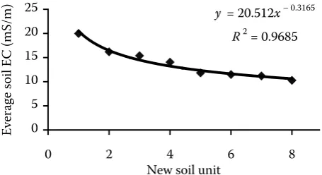
The soil EC map on Figure 5 shows the spatial distribution of the measured values. This map was created by the Kriging interpolating method which uses the weighted area, when the weights of the individual values give the variogram parameters. From the visual comparison of the main soil units distribution map and the soil conductivity map, some identical zones are obvious. The data, created by interconnection of the corresponding geo-refe-renced soil EC and BPEJ values, were further ana-lysed by means of Pearson correlating coefficient. The average soil EC values were calculated for the individual main soil units. The R2 _{coefficient reached} the value of 0.9585. The following Figure 6 shows the correlation relation between the main BPEJ soil units and soil EC values.

The correlation grade between the soil EC values and the main soil unit of the code shows a strong

dependency. The soil EC values describe well the land soil variability, which is obvious from the cor-relation coefficient level.

CONCLUSION

The soil EC measurement shows the actual land variability, and this monitoring is cheap and quick. As the analysis results shows, the BPEJ data are usable in the precise agriculture system for the decision process support. The BPEJ values have many positives because they characterise the lands according to their reproductive capabilities. By their use, e.g. by the production zones determining, it is necessary to keep in mind that the agricultural lands can be devastated on some tracts, either by their assemblage, by the wind and water erosion, or by other influences. It is therefore necessary to interpret the possible differences also in the con-text of the land historical evaluation knowledge. As an important way for obtaining the information concerning the surface area variability of the soil conditions in the frame of the whole land, the land electrical conductivity measurement can be con-sidered. Many authors, as (Sudduth et al. 1994; Jaynes et al. 1995; Kitchen et al. 1998) refer to the concrete possibilities of the soil EC data use for determining the productive zones and to manage the lands productivity. The soil EC maps cannot determine which input quantity should be applied on various land parts, but they may display and identify the soil differences on the land, which is important both for the sampling places destined for soil samples analysis, and for the productive zones determination.

Figure 5. Map of soil elec-trical conductivity (EC)

y = 20.512x– 0.3165 R2 _{= 0.9685}

0 5 10 15 20 25

0 2 4 6 8

New soil unit

Everage

soil

EC

(mS/m)

Figure 6. Chart of correlation of the average soil electrical conductivity (EC) values with the main BPEJ soil units

Soil EC (mS/m)

References

Doerge T., Kitchen N­.R., Lund E.D. (2007): Soil Elec-trical Conductivity Mapping. Available at http://www. ppi-far.org/ppiweb/ppibase.nsf/b369c6dbe705dd1385 2568e3000de93d/ c9adc4debd1cf45c852569d700636eda/ $FILE/SSMG-30.pdf (accessed March 15, 2007)

Farahani H.J. (2007): Soil Electrical Conductivity Mapping of Agricultural Fields. Available at http://www.extsoilcrop. colostate.edu/N­ewsletters/2002/Sensors/SoilEC.htm# EC (accessed March 15, 2007)

Franzen D. (2007): Yield Mapping. Available at http://www. ag.ndsu.edu/pubs /plantsci/soilfert/sf1176-3.htm (accessed March 15, 2007)

Jaynes D.B., Colvin T.S., Ambuel J. (1995): Yield mapping by electromagnetic induction. In: Proc. 2nd _{Int. Conf.}

Site-specific Management for Agricultural Systems, March 27–30, 1995, Madison, 383–394.

Kheiralla A.F., Yahya A., Zohadie M., Ishak W. (2004): Modelling of power and energy requirements for tillage implements operating in Serdang sandy clay loam, Malay-sia. Soil and Tillage Research, 78: 21–34.

Kitchen N­.R., Sudduth K.A., Drummond S.T. (1998): Development of within-field management zones: soil sur-vey versus a quantitative measure. In: Proc. 4th _{Int. Conf.}

Precision Agriculture. July 19–22, 1998, Minneapolis, 153–157.

Kumhála F., Kroulík M., Prošek V. (2001): Yield mapping of forage in mowing machines. In: Proc. Infosystems in Ag-riculture. Seč, Help-Service-Education, Prague, 65–71. Lotz L. (2007): Yield monitors and maps: Making decisions.

Available at http://ohioline.osu.edu/aex-fact/0550.html (accessed March 21, 2007)

Melchiori R.J.M., Barbagelata P.A., Christiansen C., Von Martin A. (2007) : Manejo Sitio Específico de N­itrógeno en Maiz: Evaluación del N­-Sensor. Available at http://www.agriculturadeprecision.org/mansit/Mane-joSitioEspecificoN­enMaizN­Sensor.htm (accessed May 18, 2007)

Sudduth K.A., Kitchen N­.R., Hughes D.F., Drummond S.T. (1994): Electromagnetic induction sensing as an indica-tor of productivity on claypan soils. In: Robert P.C., Rust R.H., Larson W.E. (eds): Proc. 2nd _{Int. Conf. Site-Specific}

Management for Agricultural Systems, March 27–30, 1994, Minneapolis, 671–681.

Thylén L., Jürschnik P., Murphy D. (1997): Improving the Quality of Yield Data. Precision Agriculture. BIOS Scientific Publishers Ltd., Oxford, 743–750.

Van Bergeijk J., Goense D., Speelman L. (2001): Precision agriculture soil tillage resistance as a tool to map soil type differences. Journal of Agricultural Engineering Research,

79: 371–387.

Received for publication August 1, 2007 Accepted August 29, 2007

Abstrakt

Mimra M., Kroulík M., Altmann V., Kavka M., Prošek V. (2008): Analýza vztahu mezi hodnotami elek-trické vodivosti půdy a hodnotami bonitovaných půdně ekologických jednotek. Res. Agr. Eng., 54: 130–135. Tento článek popisuje výsledky analýzy vzájemného vztahu mezi elektrickou vodivostí půdy a BPEJ (bonitovanými půdně ekologickými jednotkami). Měření byla provedena v roce 2006 na pozemku Školního zemědělského podniku v Lánech, který patří České zemědělské univerzitě v Praze. Elektrická půdní vodivost byla měřena kontaktní metodou pomocí senzoru se šesti elektrodami. N­aměřená data půdní vodivosti byla srovnávána s daty získanými z map BPEJ. Cílem bylo ověřit, zda existuje vztah mezi půdní elektrickou vodivostí a hodnotami BPEJ. Dosažené výsledky ukazují, že existuje silná závislost mezi hodnotami hlavní půdní jednotky kódu BPEJ a půdní elektrickou vodivostí. Získané poznatky lze využít v systému precizního zemědělství pro zlepšení rozhodovacího procesu.

Klíčová slova: elektrická půdní vodivost; klasifikace půd; variabilita půdy

Corresponding author:

Ing. Mroslav Mimra, Ph.D., Česká zemědělská univerzita v Praze, Technická fakulta, katedra využití strojů, Kamýcká 129, 165 21 Praha 6-Suchdol, Česká republika