Radiofrequency analysis using optical signal processing

(1)

RADIOFREQUENCY ANALYSIS USING OPTICAL

SIGNAL PROCESSING

W. N. Dawber

A Thesis Submitted for the Degree of PhD

at the

University of St Andrews

1991

Full metadata for this item is available in

St Andrews Research Repository

at:

http://research-repository.st-andrews.ac.uk/

Please use this identifier to cite or link to this item:

http://hdl.handle.net/10023/15035

(2)

Radiofrequency Analysis Using Optical

Signal Processing

A thesis presented by W. N. Dawber B A(Oxon), MSc

to the

University of St. Andrews in application for the degree of

Doctor of Philosophy April 1991

(3)

ProQuest Number: 10166560

INFORMATION TO ALL USERS

The quality of this reproduction is dependent upon the quality of the copy submitted.

In the unlikely event that the author did not send a com plete manuscript and there are missing pages, these will be noted. Also, if material had to be removed,

a note will indicate the deletion.

uest

ProQuest 10166560

Published by ProQuest LLO (2017). Copyright of the Dissertation is held by the Author.

This work is protected against unauthorized copying under Title 17, United States C ode Microform Edition © ProQuest LLO.

ProQuest LLO.

789 East Eisenhower Parkway P.Q. Box 1346

(4)

Declaration

I hereby certify that this thesis has been composed by me and is a record of work done by me and has not previously been presented for a higher degree.

This research was carried out in the Physical Sciences Laboratory of St. Salvator's College, in the University of St. Andrews, under the supervision of Dr. A Maitland.

I was admitted to the Faculty of Science of the University of St. Andrews under Ordinance general number 12 in October 1987 and as a candidate for the degree of PhD in October 1988.

(5)

Certificate

I certify that W. N. Dawber has spent nine terms at research in the Physical Sciences Laboratory of St. Salvator's College, in the University of St. Andrew's, under my direction, that he has fulfilled the conditions of ordinance No. 16 ( St. Andrews ) and that he is qualified to submit the thesis in application for the degree of Doctor of Philosophy.

(6)

Acknowledgements

I would like to tliank Dr. Arthur Maitland for his guidance and encouragement throughout this work and to Peter Hirst and Brian Condon for many helpful discussions. I am particularly grateful to the Admiralty Research Establishment for financial support and to my industrial supervisor Dr. Phil Sutton for his enthusiasm, help and interest in the project.

(7)

Dedication

(8)

_

A.2.2 LONG-PULSE CASE...247

Appendix 3

(15)

Abstract

The basic form of conventional electronic and acoustooptic radiofrequency spectrum analysers is described. The advantages and disadvantages of the various systems are discussed with particular reference to radar signal processing in a hostile environment.

Acoustooptic interaction is described using electromagnetic wave theory and also in terms of particle dynamics. A discussion of the various factors which effect Bragg-cell performance is presented, together with experimental results from the characterisation of acoustooptic cells.

Coherent light detection is described when used in conjunction with a Bragg-cell spectrum analyser. Using this approach the dynamic range of the device may be dramatically increased. A novel approach is described which uses optical fibres in the Fourier transform plane and fusion spliced couplers to combine the signal and local oscillator beams. Experimental results are presented using single-mode fibres.

Improvements in diffraction efficiency, reduced material intermodulation and increased frequency resolution are possible in an acoustooptic spectrum analyser if a Bragg-cell with a long transducer is used. However this leads to reduced instantaneous bandwidth in a conventional configuration. Two new approaches are described which allow a long transducer to be used without loss of bandwidth.

(16)

Abstract________________________________________________________________9^

magnitude by placing it within a passive cavity. Various cavity configurations are analysed and experimental results are given.

A temporal analysis of light diffracted from radiofrequency pulses within an acoustooptic Bragg-cell is presented. Experimental evidence backs up the theory, which shows a possible means of eliminating the "Rabbit’s Ears" phenomenon.

Conventional acoustooptic Bragg cells have bandwidths limited by the acoustic losses in the crystals used for the cells and impedance matching of the transducer to the driver and crystal. Commercial cells are available with bandwidths of several gigahertz.

Many applications require significantly larger bandwidths than are offered by conventional Bragg cells. We describe a new kind of diffraction cell with a potential bandwidth in excess of fifty gigahertz. The theory of operation and an example design are presented.

(17)

Glossary

a(x) Optical cell aperture function

Amplitude of optical signal electric field strength A2 Amplitude of optical reference electric field strength

B System bandwidth

B-j Relative dielectric impermeabilty of crystal

C Capacitance per unit length of TWEOD crystal c Speed of light in vacuum

Cgg Elastic constant relating stress to strain c^ Fourier component

CT^^_£^ Cross talk power between frequency channels f j and f2

D Length of TWEOD crystal in microwave propagation direction Dg System dynamic range

d Grating spacing

d^ (p,t) Fourier transform of phase modulated light entering cell d^(p,co) Transform of phase modulated light entering cell

d2(p,t) Fourier transform of phase modulated Hght entirely within cell

d2(p,co) Transform of phase modulated light entirely within cell

dg(p,t) Fourier transform of phase modulated light leaving cell dg(p,co) Transform of phase modulated light leaving cell Dj j-component of displacement current

Dpoiy Polytone dynamic range with no Hecht intermodulation

e Electronic charge

(18)

Glossary______________________________________________________________ IJ.

E ^ (0) Amplitude of un-diffracted field on entering crystal E2 Amplitude of electric field of diffracted optical wave

E2(0) Amplitude of diffracted field on entering crystal Ey Time varying electric field of diffracted optical wave E^ Time varying E-field of un-diffracted optical wave

F Cavity finesse f^ Radiofrequency 1

Î2 Radiofrequency 2

fj^ Focal length of fibre-coupling lens Fi Focal length of collimating lens

c

Fi Focal length of transform lens T.T.

Fi Focal length of input lens in

fg Acoustic frequency

g Single-pass cavity gain

g2 Single-pass cavity gain for ray 2

H Height of acoustic column ( perpendicular to acoustooptic plane ). H^y y-component of time varying magnetic field strength of un-diffracted

optical wave

H^g z-component of time varying magnetic field strength of un-diffracted

optical wave i(t) Photocurrent

Iq Average optical power of incident wave

Optical diffracted power from TWEOD i^ Detector dark current

Incident optical power I^ Optical cavity input power

(19)

Glossary_______________________________________________________________

Inti_ 2 Relative Hecht intermodulation between and £ 2

lout Optical cavity output power ighot Shot-noise current

Jjj Bessel function of n ^ order k'^ Un-diffracted optical wavevector

k* Microwave wavevector in TWEOD

Icq Un-perturbed optical wavevector

kj Un-diffracted optical wavevector k2 Diffracted optical wavevector

kg Wavevector of Bragg-diffracted light kg Acoustic wavevector

L ’ Acoustooptic interaction length in acoustic propagation direction 1 Inductance per unit length of TWEOD crystal

L Length of cell in acoustic propagation direction Ig Illumination area of polychromatic source

N Number of channels DN Dynamic range

n Optical refractive index of crystal np Number of resolvable frequencies

P Microwave power in TWEOD crystal

Pq Un-diffracted optical power

P 2 Average un-diffracted optical power

P^(0) Average un-diffracted optical power on entering crystal P 2 _ 2 Hecht intermodulation power between f^ and f2

P2 Average power density of diffracted optical wave

(20)

Glossary______________________________________________________________ O

^max Maximum optical power before saturation of detector

?min Optical power for signal-to-noise ratio of unity Pmn Piezo-optic tensor

Pg Average power density of acoustic wave P j Average total acoustic power

P j^ Acoustic power 1 Prp^ Acoustic power 2

Prp Minimum detectable acoustic signal power min

Prp Acoustic power in Bragg cell in reference arm ^ref

Q Dimensionless parameter relating transducer size to optic and acoustic wavelengths

R Detector load resistance ^best Optimum mirror reflectance

r^ Observed linear electrooptic coefficient

S Time varying acoustic strain

s(t) Time-varying applied radioffequency amplitude

S(x,t) Phase modulation on incident plane optical wave passing through cell S/Np^ Signal-to-noise ratio for acoustic power Prp

S ^ Amplitude of acoustic strain

S^ Displacement of diffracted beam in polychromatic spectrum analyser Sgbre Horizontal displacement of input fibre

Sgbre Vertical displacement of input fibre

Smax Maximum electrical input signal power before detector saturation Smin Electrical signal power for signal-to-noise ratio of unity

SNR Signal-to-noise ratio

(21)

Glossary M 1

I

T Cell transit time

Tg Equivalent system temperature Tjjj Miixor transmission

tjj Height of TWEOD crystal

t Time

TWEOD Travelling wave electrooptic diffractor V Acoustic velocity

Vg Voltage across TWEOD crystal V Sound velocity in crystal

W Acousic depth -{t

w Acoustic depth where Q'^~ x,y,z Cartesian coordinates

Z Characteristic impedance of TWEOD crystal a Fraction of light directed into reference arm Ô Round-trip cavity loss

Ag Cavity loss at Bragg cell

Ag2 Cavity loss for ray 2 at Bragg cell

Ae e' - e

6F Frequency off-set provided by mirror mis-alignment Afg Frequency resolution

Afg ^ Acoustic frequency bandwidth

1/2

colli

Afg Loss of frequency resolution due to spectrometer grating resolution

Af Loss of frequency resolution due to collimation error ,

collimation 3

'grating

St

Akg Change in acoustic wavevector Ak„ Spread of acoustic wavevector;

H/2

A ^ Cavity loss at a mirror

(22)

Glossary______________________________________________________________ 1^

ôparasitic Round-tiip parasitic cavity loss

AcOr f Difference in angular frequency between signal and reference arms

A0 Small angular change

80 Angular mirror mis-alignment

A 01 / 2 Angular spread of acoustic propagation directions

A0^ Small change in propagation angle of acoustic wave

AO Bragg cell rotation angle e Dielectric permitivity of crystal

e' Dielectric constant of perturbed crystal

8q Dielectric permitivity of free-space

(j)(y) Phase-front retardation at y

(j)Q Amplitude of phase-front retardation (j>l Phase delay for signal arm

<t> 1 . ,(j) g Unit amplitude phase terms

(^2 Phase delay for reference arm

(})£ Fibre core diameter (j)g Optical spot diameter

Fy Rate of growth of diffracted optical wave in acoustic propagation direction Rate of growth of un-diffracted optical wave in acoustic propagation direction Fg Rate of growth of acoustic field in acoustic propagation direction

T] Diffraction efficiency per watt of TWEOD T|g Diffraction efficiency per watt of cell

Optical fibre coupling efficiency Detector efficiency

tIt Transmittance due to parasitic loss in reference arm 4 e f

(23)

Glossary __________________________________________________________ 16

K Boltzmann's constant

A Acoustic wavelength

X Free space optical wavelength |i Dielectric permeability of crystal p Spatial frequency

Pg Spatial frequency corresponding to acoustic frequency (Og Complex amplitude transmittance

X Pulse duration

tB Time-bandwidth product coj Unperturbed optical frequency

CO2 Optical angular frequency of diffracted wave

cOp Doppler shifted frequency corresponding to position p

cOrP Angular radiofrequency

cOg Acoustic angular frequency

0 Diffraction angle

0 '^ Diffraction angle outside TWEOD crystal 0 j Angle of incidence in crystal j 02 Angle of diffraction in crystal 0y Bragg angle in crystal

(24)

Introduction to Acoustooptic Spectrum

Analysers

1.1 ACOUSTOOPTIC SIGNAL PROCESSING

The applications for radiofrequency spectrum analysers, particularly Radar, [1.1, 1.2] often require monitoring a wide band of the electromagnetic spectrum with the ability to recognise desired characteristics of any signal which may appear in that band. By using this information the source and nature of the signal may then be obtained.

A high probability of intercept of transient signals over a broad frequency band, in a wide field of view, and with an environment crowded with many continuous-wave and pulsed signals is desired.

Severe problems arise when the band of interest contains a large number of signals of different frequencies, amplitudes and types of modulation. The signals may also have been modulated in such a way as to deliberately make identification as difficult as possible e.g. by using frequency hopping and spread-spectrum techniques.

(25)

Acoustooptic Spectrum Analysers__________________________________________ ^

detection of radiofrequency over a wide dynamic range with 100% probability of intercept. The acoustooptic receiver produces the power spectrum of all the signals in its band simultaneously. The signals can be intermixed, pulsed or continuous-wave and may include broadband signals such as jammers or intrapulse modulated radars.

During the last decade the availability of the laser and of cheap and efficient charged coupled device ( CCD ) detector arrays [1.8] has led to the development of a wide range of special purpose systems capable of performing functions previously accomplished by microwave and lower frequency systems but with order of magnitudes greater speed and capacity. The emmergence of integrated optics and surface acoustic wave ( S.A.W. ) [1.9-1.13] devices has enabled miniature, robust, acoustooptic systems to be produced at relatively low cost.

As well as Fourier transformation, all types of multipoint mathematical multiplication of I real and complex variables may be performed using acoustooptic signal processing

techniques. These include correlations, convolutions and combinations of these with Fourier transforms[ 1.14-1.26]. One or more functions may be inputted, and the output(s) may be in one or two dimensions.

Digital computation has the advantage over optical in that it is easy to re-program, | whereas the "program" of the optical computer is set when the optics are positioned. j

j However the optical processor does what it is designed to do at an extremely high rate.

The main feature of optical processors is that they process a large signal bandwidth in j

(26)

1.2 THE ACOUSTOOPTIC SPECTRUM ANALYSER

The acoustooptic spectrum analyser is a deceptively simple optical processor. It performs a real time Fourier transform with only four active components; a light source, a Bragg-cell, a lens and a photodetector array.

The basic acoustooptic spectrum analyser is shown in figure 1.1

Light from the laser is expanded and collimated to pass through the acoustooptic cell aperture. The acoustooptic cell consists of a transducer bonded to a block of optically transparent material, as shown in figure 1.2. Radiofrequency signals to be analysed are applied to the transducer, which creates travelling acoustic waves in the block. The waves are absorbed at the other end of the block by sound absorbing putty or similar. The acoustic waves consist of periodic compressions and rarifactions, these create periodic changes in the optical refractive index of the material in the direction of acoustic propagation.

(27)

1.3 THEORY OF ACOUSTOOPTIC DIFFRACTION

1.3.1 Qualitative treatment

There are many treatments for the solution of acoustooptic diffraction [1.27-1.37]. We will divide the problem into two regimes and solve each separately, with particular emphasis on deriving the characteristics relevant in acoustooptic spectrum analysis.

Consider the case of a uniform plane wave of monochromatic light ( wavelength X/n, where X is the free space optical wavelength and n is the refractive index of the interaction medium ) incident on a column of acoustic waves consisting of sinusoidal index variations (wavelength A ) travelling at right angles to the optical beam.

Since the acoustic velocity is much less than the optical velocity we will first consider the acoustic wave to be stationary.

The light entering regions of compression experience a higher refractive index and have lower phase velocity than the light entering regions of rarefaction. As the light passes through the acoustic column the optical wavefront becomes distorted as shown in figure 1.3. Since the wave elements propagate essentially normal to the local phase front the distortion implies changes of direction for the wave elements. This leads to a redistribution of the light flux which must be considered when analysing deep ( in the direction of optical propagation ) acoustic columns. Significant simplification is possible by using approximations valid in various regions of operation.

(28)

Acoustooptic Spectrum Analysers__________________________________________

2) Shallow field ( Raman-Nath ) case. When the acoustic wavelength is comparable in size to the optical wavelength and the amplitude re-distribution may be ignored.

For condition 2 to be valid the amplitude must remain uniform across the optical wavefront. Diffraction will tend to deviate the wavefront from this condition. We shall define an acoustic depth, w, where Hght diffraction from the front of the acoustic column spreads over one cycle of the acoustic wave at the back of the acoustic column. This is shown in figure 1.3.

If the depth of the acoustic column, W, is much greater than w then we will be in the deep field regime. If the width of the acoustic column is much less than w then we are in the shallow field regime.

We define the parameter

27tW

Q _w

From figure 1.3 we see w is given by

w 0 = — and 0 = ^

2 2nA

Hence, we have

Q = ^ . 1.0

(29)

Acoustooptic Spectrum Analysers__________________________________________2

^

In practice the acoustooptic interaction is found to be predominantly Bragg-like for values of Q greater than about 10.

1.3.2 Bragg diffraction ( high-Q case )

We first analyse the case where the interaction material is isotropic and the acoustic wavefronts are plane. Following the method of Quate et al. [1.30], we shall consider the case of light incident on a column of plane acoustic waves, travelling at angle 0{ with respect to the incident hght, as shown in figure 1.4.

For the high - Q case, the acoustic waves behave very much like a crystal lattice. Light is diffracted from successive planes and diffraction takes place only at certain allowed angles of incidence ( 0{ ) and diffraction ( 0^ ), with just one diffracted beam angle giving constructive interference from successive planes.

It should be noted that the angles 0 are the angles within the material with refractive index n. If the hght enters the cell fi'om free space then the angles 0 outside the ceU will be different due to refraction at the boundaries. For near normal incidence the angles will be approximately larger by a factor of n outside the cell.

Light scattered from a given acoustic wavefront must arrive at the new optical wavefront in phase. This condition requires the angle of incidence to be equal to the angle of diffraction.

(30)

Light scattered from successive planes must arrive at the new wavefront in phase or with a path difference equal to an integral number of wavelengths. We see from figure 1.5 that the path difference for rays 1 and 2, scattered firom successive planes is

AB + BC = 2Asin0 .

To satisfy the above conditions we require

mA, = 2nAsin0,

where m is an integer. This is the "Bragg condition" for diffraction, when we have m=l.

In figure 1.6 the light is polarized with its E-vector in the plane of incidence. The figure also shows the addition of wavevectors k.2 and kg which are the incident, scattered

and acoustic wave vectors, respectively.

If the field is uniform and we neglect the coupling of the various waves, we can write for the E-field of the electromagnetic wave at angular frequency 0)j[ and travelling in the

positive z-direction as

Ei(z)

E^ = ~~Y~ exp[ i(C0jt - kjzsin0j - k^ycos0j)] + complex conjugate . 1.1

The average power density is

(31)

Acoustooptic Spectrum Analysers_____________________________________ 24

and for the wave travelling in the negative z-direction (the reflected wave)

^2(2)

Ey = —2— exp[i(C0 2t + k2zsin0 2 - k2ycos0 2)] + complex conjugate 1.3

and the average power density is

^ 2 “ 2 2% •

The sound wave may be expressed in terms of the strain, S;

S = ^ S^exp[i(0)gt - kgZ)] + complex conjugate . 1.5

The average power density in the sound wave is

P s = 5 ‘=33''sSlSl ’

where we have assumed longitudinal waves. The phase velocity of the sound wave is v^ and C 33 is the elastic constant relating stress to strain along the z axis.

From the principles of conservation of energy and momentum we have

C0i=C02+C0s 1.7

(32)

Acoustooptic Spectrum Analysers__________________________________________25

^

k i = k 2 +kg 1 . 8

The vector components of the last equation are

kisin0i+k2sin02 = kg

19

and

kicos0i = k2cos02

1.10

Since we have

cos0 ^ k2

= kj- = 1 ( approximately ), 1 . 1 1

the angle of incidence 0 i can be taken to be equal to the angle of reflection 0 2 and we

can write

(ki+k2)sin0 = ks . 1 , 1 2

This is just the Bragg condition for diffraction described earlier.

Using Maxwell's equations we have

% dHf

(33)

Acoustooptic Spectrum Analysers 26

dEf dHfj,

W “ d T 1.13

and

dHfz

dy ' dz e'. 1.14

where e' is the dielectric constant of the perturbed crystal, proportional to the strain produced in the medium by the sound wave.

Using 1.1 and 1.3 in 1.13 and performing a time integration and a spatial differentiation, we have

1 . 1 6 E j d E j 1 ,

2 * kisin0 j ^ 2 + dz ■ 2 expiKco^t - k|Sin0 ^z)) + c.c.

1.15

where we have

CO₁ ₁

which is the velocity of the unperturbed electromagnetic wave.

(34)

Acoustooptic Spectrum Analysers__________________________________________ 27

where we have assumed weak coupling,

^ « 1 .

e

We may then neglect the first term in parenthesis in 1.15. This means that the change in amplitude of Ej over a wavelength is small.

From equations 1.14 and 1.15 we have

dEi 1 1

sin0 - 2 ikjE^ exp[i(cOj^t + k2zsin0 - k^ycos0 )] + complex conjugate

■ 1-16

In order to calculate the change in permitivity,

e e

we write the relative dielectric impermeability as

dE-where kg is the unperturbed optical wavevector in the medium and the changes in B due

to strain are given by the piezo-optic tensor in the form

(35)

ABjj = PijnSn . 1.18

( We may also write the piezo-optic tensor as p ^ where m=ij ).

It is necessary to work with the full photoelastic matrix when one studies the anisotropy of the diffracted light as a function of the polarisation of the incoming light. For polarisation with the E vector in the plane of incidence and for small Bragg angles we can assume that E is parallel to the optic axis. We designate the z direction (100) as 3, the direction normal to the (1 0 0) direction and parallel to the acoustic wavfronts (y) as 2.

For cubic crystals we have the relations

^ ^ 2 ^

8 egP2 3S3 1.19

and, for light polarised in the plane of incidence along the optic axis, we have

^ ^ 1 e

g = '^ P 2 3 ® 3 - ^ - 2 0

Using equations 1.1, 1.3, 1.7, 1.9, 1.10, 1.19 and 1.20 in the right hand side of 1.16, we have

^(Ejf + Eb> = E l g Sjj^ E2

{ ^ - — P23 ■y y }exp[i(cûjt - k jzsin0 - k|^ycos0)] + c.c. + other terms. 1.21

(36)

29 Acoustooptic Spectrum Analysers

Equation 1.16 then becomes

dEi kj e S^Eg

W ^ s i n 0 Z % 3 T T • 1.22

Similarly, we can arrive at the equation for E2,

dE/) ko p S-j E-j

E23

If we assume an exponential dependence for the fields on the z-direction of the form

1.24 exp[ Fgdz] and exp[ - F^dz],

then we find

1.25 s 2 sin0

Using equations 1.22, 1.23, 1.25 and the boundary condition that E2(L')=0, we obtain

1.26

and

'2^1 sinh F_(z-L')

(37)

Therefore, at z=0 we have

^2(0) I

= i - \ I — tan h rX ' . 1.28

Ei(0) _{0 )1} s

For small values of F X this becomes

PgCO) I E 2(0) 2

Ej(0) 1.29

where we have approximated by setting

0 )1 = 0 ) 2 and = 0 2 = 0 .

If we further approximate, by setting sin0=0, then we have for the ratio of the diffracted intensity to the incident intensity

P2 ‘‘I , e ,2 1

P2 3 ] 0 2 2 V3C3 3 0

If the acoustic column has dimensions W and H, then, since the light impinges at angle

0 , the interaction length is given by

L' = Wtan0 = W 0, approximately.

(38)

Acoustooptic Spectrum Analysers__________________________________________ 3J^

P _ Z r _

and

2

^ 2 e ,2 W

P j - 8 [ P2 3] H v_{" ’'}_s'=33

1.3,2 Effect of varying the acoustic frequency

If we vary the acoustic frequency Wg so that kg changes to kg + Akg, the diffracted intensity will change.

Equation 1.8 becomes

ki+k2 = ks+Aks 1.32

( Akg is in the same direction as kg )

and in component form, equation 1.9 becomes

kjsin0j + k2sin02 = k^ + Ak^ . 1.33

We replace equation 1.1 with

1.31

(39)

—

where we have

Ak„

* '’1 " 1^1 ■ 2SÎÏ0 ’ 135

with a similar expression for Ey. This then leads to a more general form for equations 1.22 and 1.23;

* ^ 1 . . ^ 1 E ^1 %

- ^ + 1 — E i = i ^ ~ P 2 3 - ^ ^ 1.36

0

dE/) Ak k-) p Si El

W - l - f E 2 - l A - P 2 3 T T • 137

0

We assume solutions of the form

exp[Tyz] and exp[ - Eyz], 1.38

then equation 1.25 becomes

= • 1-39

The diffracted power may be obtained as before and equation 1.29 becomes

PjCO) 0 ) 2

P l ( 0 ) t O j + r ^ s i n h ^ F h L ' 1.40

(40)

Acoustooptic Spectrum Analysers__________________________________________ 3 ^

Using equation 1.39, 140 becomes

p ,,o , » ,

Pi(0) - „ , ■

1 Ak ^ / Ak ^

l - ( ^ ) ^ + s inh 7 |r , L " ^ )

Ak

For small values of Fg (weak coupling),— ^ can be much greater than unity and we can

2Fg

approximate equation 1.41 by the relation

gAkg Pn(0) (On « s in ^ -^ L ’

( ^ L ' ) 2

1.3.3 Bandwidth for a fixed angle of incidence

From equation 1.42 we see that the FWHM of the diffraction pattern as the acoustic wavevector is changed is given by

But we have

27tf_

(41)

^

Also we may write

L' = W 0 1.46

and

(ki+k2)sin0 = kg _ 1.47

Therefore, for small 0 we may write

kg

® "2kj 1-48

and

0 = X • _2nA 1.49

From equations 1.45, 1.46 and 1.49 we obtain the instantaneous radiofrequency bandwidth ( FWHM )

2nVj

(42)

We have found the variation of diffraction efficiency with frequency for a fixed angle of incidence. We now wish to find the variation of diffraction efficiency as the angle of incidence, 0 ^, changes.

As the RF frequency changes, the acoustic wavelength changes and the correct angle of incidence ( equal to the Bragg angle ) changes.

From equation 1.49, we obtain

A0 = - ^ A A 1.51

2nA^

and therefore we can write

Akj = ^ A 0 . 1.52

A.

Equation 1.42 becomes

1.53

From equation 1.53 we see that the FWHM of the diffraction efficiency as a function of Bragg-cell rotation, A0, is

(43)

Acoustooptic Spectrum Analysers__________________________________________ 3jS

provided that we have ^0 i/2 « 0 •

The FWHM is just the angular spread in acoustic propagation direction due to acoustic diffraction at the transducer. There is a set of acoustic waves over a range of angles A0 1 / 2 available for diffraction of the optical beam. This is shown on the phase matching

diagram, figure 1.7.

1.3.5 Phase matching diagrams

Phase matching diagrams are a graphical method of representing the Bragg condition ( equation 1.32 ) in momentum space. We shall show that phase matching diagrams may be used to obtain the bandwidth of an acoustooptic spectrum analyser. This is particularly useful for diffraction in anisotropic media ( see 1.3.6 ). Figure 1.7 shows the phase matching condition over the angular spread, A0 ^ , of acoustic wave-vectors.

From figure 1.7, we see that

But from 1.54, we have

A0 ^ = A0 y2 = ^

and, hence, we obtain

2kA

(44)

But we have

2icf

Vs = l E f 1-37

and

27cAf„

Ak ^ . 1.58

® ''s

From 1.56 and 1.59 we have

2nVg

"^^'1/2 = ^ ’ 1-3^

as before.

1.3.6 Bragg diffraction in an anisotropic material

Figure 1.8 shows the phase matching condition for Bragg diffraction in an anisotropic material. The incident and diffracted wave vectors lie on different index ellipsoids and are of orthogonal polarisation states. The acoustic wavevector is k^. The acoustic vector

does not meet the index ellipsoid tangentially.

(45)

when the acoustic vector meets the index ellipsoid of the diffracted wave vector tangentially.

The phase matching criterion is then met, approximately, over a range of angles. In this way the usable bandwidth for a given angle of incidence is increased.

Figure 1.10 shows the tangential phase matching condition in an anisotropic material over the angular spread of acoustic wavevectors, A0 ^.

We will assume that the anisotropy is small so that we have Ik^j « Ik2l.

We then obtain

Ak

A0 ^ = k2 ( l “CosA0 ^ ) and tanA0 ^ = - ^ . 1.60

For small we obtain

Akg = '\j2kgk2A0 ^ . 1.61

From 1.54 and 1.61 we have

V

47tk2

and from 1.58 and 1.62 the bandwidth is

(46)

Clearly, can be much larger in this case than in the isotropic case ( 1.50 ),

allowing the usable bandwidth to be limited by the transducer bandwidth rather than the phase matching criterion for a fixed light input angle.

1.3.7 Theoretical analysis of shallow field ( Raman-Nath ) acoustooptic diffraction

In the shallow field ( Q « 1 ) approximation, the amplitude of the optical wavefront remains uniform and we may represent the acoustic field as a complex amplitude transmittance, given by

where (j)(y) is given by

4>(y) = ^ • 1-65

An is the amphtude of the index variation produced by the acoustic wave.

The diffraction pattern produced by the acoustic wave is given by the Fourier transform of the amplitude transmittance ( 1.65 ) with the variable Y = ^ replacing y. Since is

(47)

A(0) = , 1.66

where c^ is given by

MIX

• 27tnYA _{cos———expj i())QCOs—^ — I'd Y .}L 2tiYA1,,, _1.67

-MIX

By substituting

in equation 1.67, we obtain

^n " ^ ^n (^0^ n = ...-1,0,1,2,... _X 1.69

Equation 1.66 represents a series of diffracted waves travelling in the directions 0^

given by

0 „ = ^ . 1.70

This is shown schematically in figure 1.11.

The Fraunhofer diffraction pattern therefore consists of sharp lines in the directions 0^

(48)

Acoustooptic Spectrum Analysers__________________________________________41^

This calculation was carried out for an infinite length acoustic column. For finite apertures, the lines will be angle-broadened by diffraction from the aperture.

1.4 EXPERIMENTAL VERIFICATION

1.4.1 Characterisation of a low-Q LiNObg Bragg-cell

1.4.1.1 Experimental layout

The apparatus is shown in figure 1.12. The ccd array is a Reticon 'K' series with 1024 elements on 25 pm centres. The Bragg-cell is a GEC Marconi Research centre Identity Y347251, SRC no.MRQ IS0Q3, driven from a radiofrequency signal generator and amplifier, with a power monitor connected in parallel.

The Bragg-cell is fabricated from LiNbOg with a refractive index, n = 2.2, and acoustic velocity, Vg = 6600 m/s.

The Bragg-cell produces an acoustic column approximately 1mm * 20mm and about

1 0mm thick in the direction of optical propagation.

(49)

acoustic beam. This provides good matching of the acoustic and optical beams. The beam is then passed through the Bragg-cell. The diffracted light is re-collimated and focused onto the ccd array. The Bragg-cell is mounted on a rotation stage which allowed movement in the 2 axes perpendicular to the optic axis, as well as rotation in the plane of

the acoustic beam.

Rotation of the Bragg-cell is measured by reflecting light from a Gre-Ne laser using a mirror mounted on the cell. The reflected light falls on to a distant graduated scale.

1.4.1.2 Diffraction efficiency as a function of radiofrequency power

The radiofrequency power applied to the cell is varied, having optimised the diffracted beam intensity ( first order ), at 118 MHz. The output is monitored on the oscilloscope,

being careful not to saturate the ccd array, by using graded neutral density filters.

The results are shown in figure 1.13.

1.4.1.3 Diffraction efficiency as a function of ceil misalignment

The experiment is repeated with the radiofrequency power set at 200mW. The cell is rotated in the plane of the acoustic beam and the relative diffracted power, in the first order, measured as before. The results are shown in figures 1.14 and 1.15.

1.4.1.4 Variation in diffraction efficiency with frequency

(50)

Acoustooptic Spectrum Analysers__________________________________________ 43

frequency, and then the experiment was repeated holding the Bragg-cell fixed. The results are shown in figure 1.16.

The open squares are the points taken with re-alignment between each reading. The closed squares were taken with the cell optimally aligned at 120 MHz.

1.4.1.5 Variation of resolution with aperture illumination

The output from the ccd array was photographed, with a 'scope camera, with an adjustable stop in front of the Bragg-cell, so that the cell was illuminated by a truncated Gaussian profile. The results are shown in figure 1.17.

Figures 1.17a to 1.17d show the increase in full width at half maximum ( FWHM ) as the aperture is closed down at 120MHz. The side lobe structure also becomes more

pronounced as the aperture is closed. The FWHM with the aperture fully open is approximately 125pm. Figure 1.17e shows the side lobe structure in more detail, with the central maximum off-scale. Figure 1.17f is taken at 70MHz with the aperture open

and has an FWHM of approximately 75pm.

1.4.1.5 Comparison of results with theory

The diffraction efficiency of the cell is approximately linear with the applied

(51)

The diffraction efficiency as a function of angular misahgnment is given theoretically by equation 1.53, for small A0.

P z C O ) Wn O ' ? j c W

A0] 1.53

This clearly doesn't fit the data in figures 1.14 and 1.15 very well. The central maximum is about the same width as the side lobes, rather than being twice as wide, as implied by the above formula. Equation 1.53 assumes operation in the Bragg regime. We show below that this is not entirely valid for this cell.

If we just take account of the position of the first minimum in the angular distribution

then we obtain a value for the length of the transducer. From equation 1.53 the first minimum occurs at an angular misalignment given by

^®min“ W

We see from figure 1.14 that the first minimum occurs at an angular misalignment of 0.01 rad. Inside the cell the angle AO^^ will be n - times smaller. We have

^9min = ^ > 1-73

and hence we obtain

W = 12 m m .

(52)

Q = 7,2 .

The value for the cell is therefore operating in a regime which is between the Bragg and

Raman-Nath regimes.

There is little difference between the two sets of results for alignment at the centre frequency and alignment at the operating frequency ( figure 1.15 ). If this cell were used in a conventional acoustooptic radiofrequency spectrum analyser, then the usable

bandwidth would be limited by the piezo-electric coupling efficiency, rather than a lack of

tracking of the Bragg angle.

The frequency resolution in figures 1.15 is consistent with diffraction at the aperture, the width of the central maximum being of the order, A0 = X7D, where D is the illuminated aperture.

1.4.2 Characterisation of a high-Q Bragg-cell

The experimental characterisation procedure has been repeated using a high-Q Bragg-cell.

The Bragg-cell is a "Automates et Automatismes" A.A. DTXIOO, fabricated in TeÛ2

with refractive index n = 2.26 and acoustic velocity v^ ( slow shear wave ) = 800m/s.

(53)

Acoustooptic Spectrum Analysers__________________________________________ £6

polarised in the orthogonal state the phase matching is "normal", as described in section 1.3.5. The phase diagram for the "normal" coupling is shown in figures 1.18 and 1.19.

1.4.2.2 Diffraction efficiency as a function of radiofrequency power

Figure 1.20 shows the variation of diffraction efficiency with radiofrequency power.

1.4.2.3 Diffraction efficiency as a function of cell misalignment

Figure 1.21 shows the variation of diffraction efficiency with cell misalignment at 134 MHz.

The angular separation of the maximum and first minimum is 0.005 rad. The FWHM is 3.5 mrad.

1.4.2.4 Variation in diffraction efficiency with frequency

Figures 1.22 and 1.23 show the variation of diffraction efficiency as the radio frequency is changed, with the laser light polarised for "normal" and "tangential" type phase matching, respectively. The Bragg-cell is aligned for optimum diffraction efficiency at 126 MHz.

The Bandwidth ( FWHM ) of the cell for "normal" phase matching is 6.4 MHz

(54)

Acoustooptic Spectrum Analysers__________________________________________ 4%

1.4.2.5 Comparison of results with theory

The position of the first minima of diffraction as a function of cell angular misalignment implies a transducer length of ( from 1.70 )

W = 1.74

^®min

W = 2.6 mm

and from equation 1 .0 we have

Q=128

From figure 1.19 we calculate the bandwidth for the "normal" phase matching. Equation 1.55 becomes

and we obtain

(55)

The measured value for the bandwidth is 6.4 MHz in good agreement. It should be noted that this is half the bandwidth that would have been obtained for an isotropic interaction of the same Q.

1.5 CONCLUSION

The basic form of conventional acoustooptic radiofrequency spectrum analysers has been described.

(56)

detector array beam expander

laser

C3

A O cell

f.L lens

Figure 1.1

incident light

applied radiofrequency signal

transducer

dif fir acted light

transmitted light

(57)

Acoustic wave

Diffracted light from front of acoustic column

Incident

Plane optical phase front

; Back of ; acoustic J column Front of

acoustic column

Transducer

Figure 1.3

(58)

Figure 1.5

diffracted light

acoustic wave

incidrat

(59)

X

2

k

Ak,

Figure 1.7

(60)

Figure 1.9

A0,

Ak,

(61)

incident light

applied radiofrequency signal

transducer

2nd order

1st order

0th order

(62)

if

n . i filter

m i r r o r s

c.c.d. a ray

Brag^ cell rotation sta ge

focussing 1er collimating lens

irror mounted on Bragg cell

se a e

cylindrical lens

He-Ne laser

G re-Ne laser

(63)

2Q

le

0 1 0 0 200 300

R.F. frequency power ( mW )

Figure 1.13

1.0

-- 0.6-

I

O n A

-5

o

0.1

0.0

-0.3 -0.2 -0.1 0.0 0.2

Angular misalignment ( rad. )

(64)

I

1.2

1.0

0.8

0.6

0.4

0.2

JÜL

0.0

0.1 0.2

0.0

Angular missalignment ( rad. )

Figure 1.15

0.8

-^ 0.6

-0.4

0.2

0.0

40 60 80 100 1 2 0 140

R.F. frequency ( MHz )

(65)

(a) 1.5mm, 120 MHz (b) 3mm, 120 MHz

(c) 5mm, 120 MHz (d) No Stop, 120 MHz

(e) 5mm, 120 MHz (f) No stop, 70 MHz

20um

(66)

Figure 1.18

Ak

(67)

A

y

10 20 30

R.F. power ( mW )

40 50

Figure 1.20

Angular missalignment (mrad)

(68)

120 122 124 126 128 130 132 134

Figure 1.22

I

d

u

124 126 128 130

(69)

1.5 REFERENCES

[1.1] ’’Antennas and receivers for EW systems" R. Kyle

Conf. proc. Miltary Electronics Defence Expo, 408-13,1978

[1.2] "Acoustooptic spectrum analyser for laser radar applications" C. Williams, M. Jennings

Proc. SPIE Int. Soc. Opt. Eng. (USA) vol. 663, 159-65, 1986

[1.3] "E.W. receivers using acoustooptic and ultrasonic components" J. Tsui, W.Brumfield

IEEE Ultrasonics Symposium Proc. vol. 1, 345-50, 1984

[1.4] "Acoustooptic techniques for real time SAR imaging"

M.Honey, D.Psaltis

Proc. SPIE Int. Soc. Opt. Eng. (USA) vol. 545, 108-17, 1985

[1.5] "Channelised integrating ESM receivers using a Bragg-cell" R. Bowman

lEE Proc. F (GB) vol.132, no.4 , 275-9 July 85

[1.6] "Optical processing of pulsed Doppler and FM stepped radar signals" D. Casasent, F. Casasayas

AO Vol. 14, No. 6, 1364, Jun 75

(70)

Acoustooptic Spectrum Analysers__________________________________________6 ^

H. Stark, F. Tutteur, M. Sayar

AO Vol. 10, No. 12,2728, Dec 71

[1.8] "Acoustooptc spectrum analysis of radar signals using an integrating photodetector array"

J. Lee

A.O. vol. 20, No. 4 , 595-600, 15 Feb 81

[1.9] "Acoustooptic interaction for most effective deflection of unguided light via acoustic surface waves"

A. Alippi, A.Palma, L.Palmieri, G.Socino

AO Vol. 15, No. 10, 2400-2404, Oct 76

[1.10] "Surface wave acoustooptic signal processors" N. Berg, J.Lee, B.Udelson

Optical Engineering Vol. 19, No.3, 359-369, May 80

[1.1 1] "Integrated optics: a tutorial review"

P. Layboum, J. Lamb

The radio and electronic engineer. Vol. 51, No. 717, 397-413, Jul 81

[1.12] "Tliin film travelling wave light modulator

A. Attard

(71)

Acoustooptic Spectrum Analysers__________________________________________ 64^

[1.13] "Time integrating acoustooptic correlator"

R. Sprague, C. Koliopoulos

A.O. Vol. 15, No. 1, 89-92, Jan 76

[1.14] "Multi channel optical correlator for radar signal processing" D. Casasent, E. Klimas

A.O. vol. 17, No. 13, 2058-2062, July 78

[1.15] "Acoustooptic implementation of real and near real time signal processing" N.Beag, J.Lee, W,Cassaday

Optical Engineering Vol. 18, No. 4, 420-428, Jul 79

[1.16] "Squared signal correlation and a possible acoustoptic implementation"

A. Goutzoulis and V. Vijaya Kumar

AO Vol. 23, No. 6, 798-802, Mar 84

[1.17] "Optical correlation of Fresnel images" G. Meltz, W.Maloney

AO Vol. 7, No. 10, 2091-2099, Oct. 6 8

[1.18] "Optical image correlation using acoustooptic and charge coupled devices" D.Psaltis

(72)

[1.19] "Fresnel diffraction by a semitransparent straight edge object with acoustically coherence controllable illumination"

Y.Ohtsutka, Y.Mei Cheah

AO Vol. 23, No. 2, 300-306, Jan 84

[1.20] "Frequency multiplexed and pipelined iterative optical systolic array processors" D. Cassasent, J.Jackson,C.Neuman

AO Vol. 22, No. 1, 115-124, Jan 83

[1.21] "Correlator based on an integrated optical spatial light modulator" C.Verber, R.Kenan,J.Busch

AO Vol. 20, No. 9, 1626-1629, May 81

[1.22] "Hybrid time and space integrating processors for spread spectrum applications" G.Silbershatz, D.Cassasent

AO Vol. 22, No. 14, 2095-2103, Jul 83

[1.23] "Adaptive optical processor"

A.VanderLugt

AO Vol. 21, No. 22, 4005-4011, Nov. 82

[1.24] "Systolic time integrating acoustooptic binary processor"

A.Goutzoulis

(73)

[1.25] "Incoherent spatial filtering with a scanning heterodyne system" G.Inbetouw and Ting-Chung Poon

AO Vol. 23, No. 224,4571-4574, Dec 84

[1.26] "Characteristics of acoustooptic devices for signal processors" I. Chang, D. Hecht

Optical Eng. Vol. 21, No. 1, 076-081 Jan 82

[1.27] "Acoustooptic signal processing" Berg, Lee

Marcel Dekker inc ISBN 0-8247-1667-12

[1.28] "Acoustooptics" J. Sapriel

John Wiley and sons ISBN 0-471-99700-5

[1.29] "Ultrasonic signal processing"

A. Alipi

World Scientific ISBN 9971-50-864-8

[1.30] "Interaction of light and microwave sound"

C.F. Quate, C.D. Wilkinson and D.K. Winslow

AO vol. 53 No. 10, Oct 65.

[1.31] "Electromagnetic propagation in periodic stratified media. I. General theory" P. Yeh, A. Yariv and C. Hong

(74)

Acoustooptic Spectrum Analysers__________________________________________ 67^

[1.32] "Optical spectrum analysis of large space bandwidth signals" C. Thomas

AO Vol. 5, No. 11, 1782-1790, Nov 6 6

[1.33] "Optical considerations for an acoustooptic deflector" L.Dickson

AO V ol.ll, No. 10, 2196-2203, Oct 72

[1.34] "Performance and optical characterisation of efficient wideband gallium phosphide Bragg cells"

R.Bonney, O.Zehl, J.Rosenbaum, M.Price AO Vol. 23, No. 16, 2778-2783, Aug 84

[1.35] "Matrix formalism for the analysis of acoustooptic beam steering" R.Pieper, A.Korpel

AO Vol. 22, no. 24, 4073-4081, Dec 83

[1.36] "Bragg-cell diffraction patterns"

A. Vander Lugt

AO Vol. 21, No.6, 1092-1100, 15 Mar 82 .

[1.37] "Simple acoustic modulators" J.Hamer, D.Channin

(75)

Coherent Detection in an Acoustooptic

Spectrum Analyser using Optical Fibres

2.1 INTRODUCTION - COHERENT DETECTION

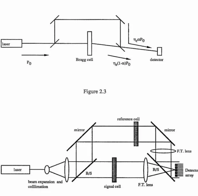
In order to increase the dynamic range of an optical detector, the optical signal to be measured may be heterodyned with a second, reference, signal at a slightly different frequency before falling on to the detector ( see figure 2.1 ). The resultant signal from a power ( square law ) detector will contain a component at the difference frequency. We have for the power at the detector

P = ( E j + E2 ) ( E j + E2 )* 2 . 1

where E%, 5% are the electric fields of the signal and reference beams, given by

Ej = A^expLKcûQt + (j)^] 2 . 2

and

E2 - A2exp[i(cûQt + coj^t + (j)2)] 2.3

and where

A \, A% = amplitude of electric fields.

(76)

Coherent Detection______________________________________________________ 69

Then we have for the light power falling on the detector

P ={ A^exp[i(cûQt + 4>i)] + A2exp[i(CDQt + coj^pt + <j)2)] } { A^exp[ - i(coQt + (j)^] +

A2exp[- i(CûQt + Wgpt + ())2)] } 2.4

Which we write as

2 2

P — Aj^ + A2 "t" 2Aj^A2Cos( tOppt + (j)2 - 2.5

The first two terms are the normal "incoherent" terms, proportional to the square of the incident E-fields. The third term is a component at the difference frequency whose magnitude is proportional to the amplitude of the signal E-field.

This has important consequences for pre-detector signal processing in that it allows the dynamic range of a system to be greatly improved. Consider a system using ( square law ) detectors with a dynamic range of DN dB. We have

P

D N =1 0 1o g j f ) ( - ^ ) 2 . 6

m in

where Pmax ^min the maximum and minimum powers measurable by the detectors.

(77)

Coherent Detection______________________________________________________ 7 ^

We have

S

D c = 1 0 1 o g , o ( # ^ ) 2.7

"^min

In a system using non-coherent detection, the signal power, S, is proportional to the light power, P, arriving at the detectors ( P a S). If there is enough light to saturate the detectors at large signal powers then we see from 2.6 and 2.7 that the system dynamic

range will be equal to the detector dynamic range,

Dg = DN .

For a system using coherent detection the signal is proportional to the amplitude of the incident light, P a S^, and equation 2.7 for the system dynamic range becomes

Dg = 1 0 1o g ^ o ( - ^ ) 2 . 8

^min or

p

D g = 2 0 1 o g i Q ( : ^ ) 2.9

m i n

If there is sufficient light reaching the detectors to saturate them at large signal powers

then the system dynamic range becomes ( from 2 . 6 and 2.9 ),

(78)

Coherent Detection______________________________________________________IJL

We see in the case where the detectors saturate at large signal powers then the system dynamic range is doubled (on a logarithmic scale ) by using coherent detection. For example in a conventional, incoherent, system using detectors with 30dB dynamic range, the maximum achievable system dynamic range is 30dB. The coherent system could have a 60dB dynamic range - an improvement by a factor of one thousand.

We have assumed that the ratios of the minimum to maximum detected signals are the same for the coherent and power detector systems and that there is sufficient light to saturate the detectors at In practice this is not always the case and we must look at

particular systems to evaluate the improvement in dynamic range brought about by using coherent detection.

2.2 DYNAMIC RANGE IN SPECTRUM ANALYSER SYSTEMS USING COHERENT DETECTION

We shall now look at the case where the system using coherent detection does not have enough light to saturate the detectors ( it is found that in practice this is usually the case ). In this situation the dynamic range is not necessarily doubled by incorporating coherent detection.

2.2.1 Free space reference beam

(79)

the detector therefore differ in frequency by the applied radiofrequency. There will be a component in the output from the detector at the radiofrequency, proportional to the amplitude of the field from the diffracted beam.

From chapter I we have, for the diffraction efficiency of a Bragg-cell

^ = T[^P

2 3

] ' I ^ ■

1-31

We write this as

^2 ~ ^ B ^ T ^1 * 2 . 1 0

The interferometric spectrum analyser is shown in figure 2.3. The signal and reference arm transmittances are Tjg and T|^, taking into account all losses, and the fraction of light

transmitted to the reference arm is a. Then we have, from equation 2.5, for the power reaching the detectors

= aîij. -H ( 1-a )Tig + 2 [aqj.(l-a)Tig] ^/^cos(Acoj^t + A(])), 2.11

where A co^ is the difference in frequency between signal and reference beams, A()> is the phase difference and Pq is the laser power. The signal strength is given by

(80)

where i(t) is the time varying component of the photocurrent, R is the detector load

resistance and is the detector efficiency.

The output current from the photodetectors may be written in the form

where i^ is the dark current. We have assumed the detectors do not saturate for the light

power levels involved.

The signal-to-noise ratio is then given by [2.2]

SNR=- - 'signal >

2 7

R< ighot > + Thermal noise + R<Dark current >

where is the shot noise, i^^^^ = V2eiB , and the thermal noise is 4icTgB, B is the

detector bandwidth, k is the Boltzmann constant, e is the electron charge, i is the photocurrent and T^ the equivalent system temperature. Then from 2.12 we obtain

cos^(A(|))

SNR= p--- ^ . 2.14

2eBR|PQTi^{arij.+(l-a)qg] +1^) + ^^^s®

Where we have assumed the d.c. dark current noise has been filtered-off.

(81)

Coherent Detection 7 4

a signal-to-noise ratio of unity when the system integrates the signal for a time 1/B. Equation 2.14 gives the minimum detectable signal arm transmittance, T|g .

min We have

2eBR I PqTI jttll ‘d } + 4kTjB

■'ls„i_nun„ = „ „ 2 2 i 2.15

and hence we obtain the minimum detectable signal power

2eBR P()T|dO^Tlr+ ^d} + ^kT^B

P'p . = ~— r~ r--- 2.16

' RPoT1d [aB r(l-a)] - 2eBRPQT|j(l-a)lT,BnL

where T|j^ is the transmittance in the signal arm due to parasitic losses only.

If dark current and thermal noise are the dominant sources of noise then equation 2.16 becomes

2eBRL + 4kT^B

P t . = - 9 n --- 2.16a

RPond«Br(l-«)BBBL

2.2.1.1 Effect of intermodulation

(82)

If detector saturation does not occur then the maximum signal will be limited by third- order two-tone intermodulation. This effect occurs when two or more signals ( a polytone signal ) are present and produces spurious diffracted beams.

Consider the case where we have two signals present at frequencies f and f2* The light may first be diffracted by fp This diffracted beam may then be diffracted back in to the direction of the incident beam by f2 * This corresponds to a frequency fj- f2* This

doubly diffracted beam is not usually in the frequency region of interest, it may however be diffracted again by f j giving a beam of light corresponding to a frequency 2 fy f2*

This is the third-order two-tone intermodulation. It usually is in the region of interest and is of magnitude

^1 - 2 “ ^ 0 - r j 2.17

This assumes all of the multiple diffraction processes occur at the correct Bragg angle for diffraction and that each takes place over one third of the interaction length, W ( from

equation 1.31 we see that the diffraction efficiency is proportional to W ). In a high "Q" cell the intermodulation term will be smaller due to Bragg angle mis-matches.

The relative intermodulation is given in dB by

Int^ _ 2 “ 2 . 1 8

P i

where P^is the diffraction due to f^^ alone.

Radiofrequency analysis using optical signal processing

RADIOFREQUENCY ANALYSIS USING OPTICAL

SIGNAL PROCESSING

W. N. Dawber

A Thesis Submitted for the Degree of PhD

at the

University of St Andrews

1991

Full metadata for this item is available in

St Andrews Research Repository

at:

http://research-repository.st-andrews.ac.uk/

Please use this identifier to cite or link to this item:

http://hdl.handle.net/10023/15035

Radiofrequency Analysis Using Optical

Signal Processing

uest

Contents

_

Abstract

Glossary

Introduction to Acoustooptic Spectrum

Analysers

^

^

kisin0i+k2sin02 = kg

19

kicos0i = k2cos02

1.10

^

V

2

if

I

I

I

I

d

Coherent Detection in an Acoustooptic

Spectrum Analyser using Optical Fibres

^ = T[^P

] ' I ^ ■