Auxiliary Variables for Bayesian Inference in Multi-Class
Queueing Networks
∗
Iker Perez
†1, David Hodge
2, and Theodore Kypraios
21
Horizon Digital Economy Research, University of Nottingham, Nottingham, UK 2School of Mathematical Sciences, University of Nottingham, Nottingham, UK
This is a post-peer-review, pre-copy/edit version of an article published in Statistics and Computing. The final authenticated version is available online at: http://dx.doi.org/10.1007/s11222-017-9787-x.
Abstract
Queueing networks describe complex stochastic systems of both theoretical and practical interest. They provide the means to assess alterations, diagnose poor performance and evaluate robustness across sets of interconnected resources. In the present paper, we focus on the underlying continuous-time Markov chains induced by these networks, and we present a flexible method for drawing parameter inference in multi-class Markovian cases with switching and different service disciplines. The approach is directed towards the in-ferential problem with missing data, where transition paths of individual tasks among the queues are often unknown. The paper introduces a slice sampling technique with map-pings to the measurable space of task transitions between the service stations. This can address time and tractabil-ity issues in computational procedures, handle prior sys-tem knowledge and overcome common restrictions on ser-vice rates across existing inferential frameworks. Finally, the proposed algorithm is validated on synthetic data and applied to a real data set, obtained from a service delivery tasking tool implemented in two university hospitals.
Keywords— Queueing networks, Continuous-time Markov Chains, Uniformization, Markov chain Monte Carlo, Slice Sampler
1
Introduction
Recent literature addressingqueueing networks (QNs) has aimed to study inferential methods for the estimation of service requirements. These networks offer the means to describe complex stochastic systems through sets of inter-acting resources, and have found applications in the design
∗Work supported by RCUK through the Horizon Digital Economy
Research grants (EP/G065802/1, EP/M000877/1) and The Health Foundation through the Insight 2014 project “Informatics to identify and inform best practice in out of hours secondary care” (7382).
†Corresponding author, e-mail: [email protected]
of engineering and computing systems (Kleinrock, 1976), or within call centres (Koole and Mandelbaum, 2002), factories (Buzacott and Shanthikumar, 1993) and hospitals (Osorio and Bierlaire, 2009). Enabling the understanding of service performance is very important, since it provides quantita-tive input for the optimal design of interconnected service stations. Yet, drawing inference on parameters is a chal-lenging errand, since in most applications successive net-work states are never fully observed. Hence, proposed ap-proaches often rely on reduced summaries such as queue lengths, visit counts or response times, and perform infer-ence in different ways, including regression-based estimation procedures, non-linear numerical optimization or maximum likelihood methods. For a recent review on the matter we re-fer the reader to Spinner et al. (2015) and rere-ferences therein.
In this paper, we focus on the underlying continuous-time Markov chains (CTMCs) induced by general-form open QNs, and we develop a flexible framework for drawing Bayesian inference on parameters that govern these mod-els; in the presence of general patterns of missing data cur-rently only discussed in(Sutton and Jordan, 2011). Statisti-cal computation is very difficult within this family of mod-els, as it involves working with often countably infinite state spaces where observations provide little indirect informa-tion. Here, we target multi-class Markovian cases with pos-sible class switching and different service disciplines, where few or no individual job departure times are observed at spe-cific servers. Hence, knowledge is mostly restricted to task arrival and departures times to, and from, the network. A
from techniques aimed to explore countably infinite state spaces withinDirichlet mixture modelsorinfinite-state hid-den Markov models (Walker, 2007; Van Gael et al., 2008; Kalli et al., 2011), and sits well within a uniformization ori-ented MCMC scheme for jump processes as presori-ented in Rao and Teh (2013).
Currently, common assumptions in inferential frame-works include the existence of complete data, product-form equilibrium distributions or unique classes with shared ser-vice rates. However, we often encounter systems where the completion of jobs at individual stations is only occasionally registered. In addition, inference on the basis of balance may in cases be inaccurate; for instance, the existence of equilibrium in service delivery systems with human work-ers is a strong assumption, since workload is usually ex-ternally controlled and arrivals hardly constitute a Poisson process. In addition, there exist concerns regarding the use of steady-state metrics whenever prior knowledge and con-straints are imposed on parameters (Armero and Bayarri, 1994); and the use of product-form solutions within popular
BCMP networks (Baskett et al., 1975) restricts first come first served (FCFS) queues to share service distributions over different task classes.
Aiming for flexible inferential methods, Bayesian proce-dures relying on Markov Chain Monte Carlo techniques were first explored in Sutton and Jordan (2011). There, the authors discussed a latent variable model targeting networks where only subsets of transition times are ob-served; the method was applicable to open QNs and de-fined through deterministic transformations between the data and independent service times across different disci-plines. Later, Wang et al. (2016) proposed the use of a Gibbs sampler relying on product-form distributions and queue length observations, and it advanced the study of closed BCMP networks, offering an approximation method for the normalizing constant within the network’s equilib-rium distribution. To the best of our knowledge, no fur-ther advances exist in the study of exact Monte Carlo in-ferential frameworks overcoming known restrictions in the study of QNs. Yet, significant progress has been made with sampling techniques and approximate inference meth-ods for continuous-time dynamic systems often modelled as CTMCs orcontinuous-time Bayesian networks (CTBN) (Nodelman et al., 2002; Fan and Shelton, 2008). However, simulating system dynamics conditioned on scarce obser-vations remains a complex task; a review on the efficiency of various methods for this purpose (including direct sam-pling, rejection sampling and uniformization methods) can be found in Hobolth and Stone (2009).
Recently, authors Rao and Teh (2013) have presented a noteworthy contribution based on the principles of uni-formization (Lippman, 1975; Jensen, 1953). Their work ex-plores a class of auxiliary variable MCMC methods allowing for the efficient and exact computation of state evolutions in systems with discrete support (such as Markov jump pro-cesses). The framework relies on producing highly
depen-dent time discretizations within subsequent blocked steps in a Gibbs sampler, and is hypothetically applicable to the study of system evolutions within QNs. However, such sys-tems exhibit strong and characteristic temporal dependen-cies (cf. Sutton and Jordan (2011)), transitions over an infi-nite set of states, varying specifications of service disciplines and Markovian regimes often subject to switching. Hence, we face major impediments which require elaborate imple-mentations of slice sampling techniques (Neal, 2003). In this work, we describe a method that controls the computational complexity within simulation procedures; for that matter, we employ families of auxiliary variables across steps in a Gibbs sampler targeting network paths. The result is a method that imposes strong restrictions within the vast space of permissible network transitions at each iteration; however, each subsequent step in the sampler allows for sig-nificant timing and routing deviations in limited numbers of tasks routed through the network, ensuring convergence to (i) the distribution of network path evolutions across its full space, given the evidence (ii) the posterior distribution of the arrival and service rates. Finally, we present results on both synthetic and real data, obtained from a service de-livery tasking tool implemented in two jointly coordinated university hospitals in the United Kingdom.
The rest of the paper is organised as follows. Section 2 describes CTMCs induced by general form QNs, introduces notions of compatibility with observations, and states the problem addressed in the work. In section 3 the principle of uniformization and its application to networks is briefly re-vised, mappings to task transitions and auxiliary variables are introduced and the proposed sampler is described. Sec-tion 4 introduces results for three example networks of vary-ing complexity with both synthetic and real data. Finally, Section 5 offers a brief closing discussion.
2
Queue networks and continuous-time
Markov processes
Consider an open Markovian network withM single service stations, apopulation set C of different task classes and a non-deterministic network topology defined by a family of
routing probability matrices P ={Pc:c∈ C}, such that
• Pc
i,j denotes the probability of a class c ∈ C task im-mediately moving to station j after completing a job service in stationi, for all 1≤i, j≤M.
• Pc
i,0 denotes the probability of a class c ∈ C task im-mediately exiting the network after completing a job service in stationi, for all 1≤i≤M.
• PM
j=0Pi,jc = 1, for all 1≤i≤M, c∈ C.
have constant rates, and vary over servers and classes; we denote them µci for all 1≤i≤M, c ∈ C. Switching is al-lowed and thus classes are not permanent categorizations; state-dependent service rates are not considered but follow naturally.
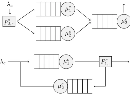
In Figure 1 we observe two example networks further ex-amined within Section 4 in this paper. There, shaded cir-cles indicate servers with exponential service rates µci, all accompanied by corresponding jobqueueingareas pictured as empty rectangles. Together, such server and queue pairs each represent a service stationi, 1≤i≤M. The shaded boxes are probabilistic routing junctions, where task des-tinations after a job service (or arrival) are determined ac-cording toPc(orpc). Finally,λ
cshow rates for exponential task arrivals from outside the network.
λc
µc1
µc 2
µc 3 pc0,·
λc µc1
µc2
[image:3.612.65.275.250.405.2]Pc 1,·
Figure 1: On top, a bottleneck network with 3 servers; bot-tom, 2 networks routed in a loop with a single entry and exit server.
Under exponential and independence assumptions, there exists an underlying continuous-time Markov processX = (Xt)t≥0that describes the system behaviour. Formally, de-noting byS the countably infinite set of possible states in the network,X is a right-continuous stochastic process such that time-indexed variablesXtare defined within a measur-able space (S,ΣS), where ΣS stands for the power set ofS.
On a basic level,X holds the ordering of jobs in each queue and server, along with their classes and task identifiers; and S is the multidimensional product of all possible congruent states at every station. Theinfinitesimal generator matrix
QofX is infinite and such that
P(Xt+dt=x0|Xt=x) =I(x=x0) +Qx,x0dt+o(dt)
for allx, x0∈ S. Elements in the generator describe rates for transitions within states in the chain, in additionQx,x0 ≥0 for all x 6= x0, and Qx := Qx,x = −Px0∈S:x6=x0Qx,x0. Hence, rows in Q sum to 0, and the full rate for a state departure is given by |Qx|, for allx∈ S. Note that tran-sition rates are the product between routing probabilities and exponential rates above; for instance,
• λcpc0,iis the transition rate among states inS account-ing for a class-carrival to service stationi,
• µc
iPi,jc is the transition rate among states inS account-ing for a job of classcserviced at stationiimmediately transitioning to stationj.
2.1 Observations
Let Γ ={0, . . . , M}2×
Ndefine atask transition space. A
tripletγ = (i, j, k)∈Γ denotes a transition for a uniquely identifiable task k, with i and j specifying the departure and entry stations respectively. Note that it is possible to augment Γ in order to include task classes, yet given unique identifiers this information is redundant. In this work, a transition triplet is never fully observed; instead, we define a set of partial observationsO=O1∪ O2⊂ΣΓ, with
O1={σ∈ΣΓ:γ1=γ10, γ3=γ30 and γ2, γ20 >0, for allγ,γ
0∈σ},
O2={σ∈ΣΓ:γ2=γ20 = 0, γ3=γ30 and γ1, γ10 >0, for allγ,γ
0∈σ},
where ΣΓ stands for the power set of Γ.
Definition 2.1. Anobservation in Ois a subset of Γ that contains all permitted task transitions in the network at some specified timet >0, given external information on an arrival, departure or job service.
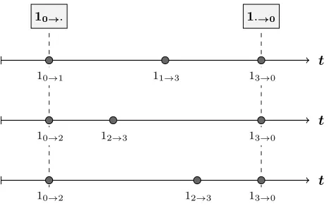
t
10→1
10→·
11→3
11→·
13→0
13→· 1·→0
Figure 2: Sample observations generated by a single task transitioning a bottleneck network with 3 servers. Obser-vations are represented by rectangles. Dots inform us of transition times. Information below the dots specifies the actual task transitions at each step.
In Figure 2 we observe a bottleneck network produce four partial observations as it evolves over time. The network corresponds to that in Figure 1 (top), and observations in-clude a single task arrival, two job services for the task, and a departure immediately after the final service. There, each task transition (i, j, k)∈ Γ is marked aski→j at its corre-sponding time point; note that indexesi, j take the value 0 in order to specify an external arrival or a departure. The observations take the form of elements ofO, i.e.
1i→·={γ∈Γ :γ1=i, γ2>0, γ3= 1} ∈ O1,
fori∈ {1,2,3}, and
[image:3.612.324.554.417.478.2]In this toy example, it is possible to deduce the original pathX in the network when considering the available ob-servations along with the topology in Figure 1; including task orderings across all queues and servers at every point in time. However, in real world applications job service ob-servations are often missing or do not exist at all. In this work, only arrivals and departures are assumed to always be available.
2.2 Compatibility
LetT :S2→Γ∪
∅define a measurable function, equipped
with the corresponding products of discrete algebras, which maps a pair of statesx, x0∈ S to its task transition triplet in Γ. For instance,
T(x, x0) = (2,3,12)
shouldx0 be reachable fromxby servicing a job for task 12 in server 2 and immediately routing it to queue 3. Note that for this to be possible, a job for task 12 must be in server 2 withinx, and the remaining tasks in the system must be distributed and ordered across stations so that there will exist full agreement with x0. If a state x0 is not directly reachable fromx, thenT(x, x0) =∅. We note that the
pre-image of a triplet inT is given by a countably infinite set of pairs of network states in S, unless bounds on the task population are imposed.
Definition 2.2. Fix some terminal time T > 0 and let {Otr ∈ O :r= 1, . . . , R} be a sequence of observations at
times 0≤t1 <· · · < tR ≤T. Also, let Ytr =T −1(O
tr)∈
Σ2S for all r= 1, . . . , R. Then, we say that a processX is
compatiblewith an observationOtr, and we writeX ⊥Otr
if
lim s%tr
Xs=y and Xtr =y 0,
for some pair of network configurations (y, y0)∈Ytr.
Fur-thermore, we say that a processX is fully compatible with the observations ifX⊥Otr for allr= 1, . . . , R.
t
t
t
10→1
10→·
11→3 13→0
1·→0
10→2 12→3 13→0
[image:4.612.54.287.542.688.2]10→2 12→3 13→0
Figure 3: Example network paths, all compatible with ar-rival and departure observations for a single task entering and leaving a bottleneck network with three servers.
In Figure 3 we observe task transitions for sample paths X which are compatible with the arrival and departure in-formation as shown in Figure 2. There, notice that the first sequence corresponds to the original path forming the ob-servations. This time, no job services have been retained and there exist infinitely many paths X that could have produced the same output, with varying transition times and task orderings across the different stations. In large networks with multiple tasks and all simultaneously transi-tioning the system, it is hard to picture the infinite amount of fully compatible pathsX, unless large proportions of job services are retrieved.
2.3 Latent network and problem statement
Denote by x0 ∈ S the initial state in X. In this paper, this is assumed to be anempty state, where no jobs popu-late the network. It is however possible to define an initial distributionπ over states, s.t. π(x) := P(X0 = x) for all x ∈ S. Now, assume we retrieve K ∈ N observation
se-quences ˜O ={Ok}k=1,...,K collected during different real-izationsX={Xk}
k=1,...,K in the network; with
Ok ={Otr ∈ O:r= 1, . . . , Rk}
at times 0≤t1<· · ·< tRk≤Tk, fork= 1, . . . , K.
The likelihood function is proportional to the product of network path densities fully compatible with ˜O, and is thus intractable. A Gibbs sampling approach centred around la-tent network evolutions is appropriate, iterating between paths and parameters. For that, note that every X is a piecewise-constant process and may be fully characterized by a set of transition times t = {t1, . . . , tn} along with network states x ={x1, . . . , xn}, so that X ≡ (t,x) with X0=x0. To ease notation, denoteθ≡(P,p,λ,µ), where
pis the vector of arrival routing probabilities. Now, letδx be the number of transitions in x excluding task arrivals and departures. For eachk= 1. . . , K, the density of (t,x) givenOk is (up to proportionality) such that
fX((t,x)|θ,Ok, x0)
∝fO(Ok|(t,x), x0)fX((t,x)|θ, x0)
∝(1−q)δx−δo×
I((t,x)⊥O:O∈Ok)
×eQxn(Tk−tn)
n
Y
i=1
Qxi−1,xie
Qxi−1(ti−ti−1), (1)
whereqdenotes the probability that a job service inXis ob-served, andδo≤δx is the corresponding amount of service observations inOk. This density is supported in a suitably defined space of finite network evolutions and the term on top is proportional to Bernoulli trials penalizing network paths with unobserved job services. The term below fol-lows from the properties of the minimum of exponentially distributed random variables.
dependencies. In the following, we revise the notion of uni-formization and sampling methods for jump processes intro-duced in Rao and Teh (2013), and we present an auxiliary observation-variable sampler fit for inference in QN models.
3
Uniformization and auxiliary
observa-tions
A generative process for sampling X requires alternating between exponentially distributed times and transitions in proportion to rates. Instead, auniformization-based (Lipp-man, 1975; Jensen, 1953) sampling scheme employs a dom-inating rate Ω and introduces the notion of virtual transi-tions, so that all times are sampled in a blocked step. In Algorithm 1 we observe a uniformization procedure to pro-duce network paths.
Algorithm 1Uniformization procedure for process X
1: Fix a dominating rate Ω≥maxx∈S|Qx|.
2: Sample transition times 0≤t1<· · ·< tm≤T from a homogeneous Poisson process with rate Ω.
3: Set initial stateX0=x0. 4: fori∈ {1, . . . , m}do
5: Samplexi from {xi−1} ∪ Xxi−1, with
Xxi−1 ={x∈ S\{xi−1}:T(xi−1, x)6=∅},
and probabilitiesπxi−1 given by
πxi−1={1 +Qxi−1/Ω} ∪ {Qxi−1,x/Ω :x∈ Xxi−1}.
6: end for
7: Return (t,x).
A proof of probabilistic equivalence between a genera-tive and uniformized sampling scheme involves comparing the marginal distribution across states at any timet ≥ 0, and can be found in Hobolth and Stone (2009). A uni-formization procedure yields an augmented set of times
t0 = {t0
1, . . . , t0m} and states x0 = {x01, . . . , x0m} that ac-counts for both real and virtual transitions inX. Whenever xi =xi−1 we refer to transition ias virtual and note that the number of such transitions is dependent on the choice of Ω. Finally, the density function in (1) may be rewritten to include virtual jumps, so that
fX((t0,x0)|Ω,θ,Ok, x0)
∝(1−q)δx0−δo×
I((t0,x0)⊥O:O∈Ok)
× m
Y
i=1 QI(x
0
i6=x0i−1) x0
i−1,x0i (Ω +Qx
0
i−1)
I(x0i=x0i−1),
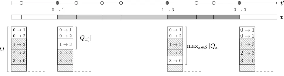
where terms not proportional to (t0,x0) are omitted. In practice, simulatingXonly requires considering a lim-ited number of candidate states in each transition; in close relation to the number of service stations. In Figure 4 we
observe a graphical representation of times, states and tran-sition probabilities for a uniformization-based procedure in the single-class bottleneck network in Figure 1 (top). There, we observe only one task from entry to departure, and we noticex0is unaltered after virtual transitions. Vertical rect-angles are divided in proportion to rates for services and arrivals, and infeasible services are hashed in grey (the ad-ditional hashed area in the bottom accounts for a strictly positive dominating rate Ω). This determines the probabil-ities leading to new states at subsequent times, with virtual jumps associated to the sum of all hashed regions. Finally, removing virtual transitions within (t0,x0) yields the desired realization (t,x) inX.
3.1 An auxiliary observation-variable sampler
A uniformization oriented approach can enable the con-struction of a Gibbs sampler targeting the conditional distri-butionfX((t,x)|θ,Ok, x0). For such purpose, authors Rao and Teh (2013) show it is possible to recycle groups of real transition times within each iteration. The method applies well to many families of Markov jump processes, but it is insufficient in order to tackle complex systems such as QNs due to a quadratic cost on the number of states when pro-ducingx. This is a known problem in discrete-time systems with large state spaces (such as dynamic Bayesian networks or infinite-state hidden Markov models), and proposed so-lutions include approximate inference methods (Boyen and Koller, 1998; Ng et al., 2002) or the use of slice sampling techniques for exact inference (Van Gael et al., 2008).
However, QNs contain strong serial dependencies, and transitions over an infinite set of states are triggered by a very reduced number of rates; hence, this can render tech-niques aimed at Dirichlet mixture models (Walker, 2007; Kalli et al., 2011) or hidden Markov models unusable. A viable approach would ideally consider limited divergences in network paths X over subsequent steps in a sampler; yet allowing for considerable deviations in the routing of a reduced set of tasks. Here, we describe a sampling scheme that achieves this goal by employing random auxiliary map-pings to the space of task transitions Γ. Intuitively:
• In each iteration we will first produce additional aux-iliary evidence, resulting from task transitions within the current trajectory ofX.
• This evidence will be used next in order to significantly restrict the explorable range of network paths in the the following sampler iteration.
t0
0→1 1→3 3→0
x0
0→1 0→2
1→3
2→3
3→0
0→1 0→2
1→3
2→3
3→0
0→1 0→2
1→3
2→3
3→0
0→1 0→2 1→3 2→3 3→0
Ω maxx∈S|Qx|
[image:6.612.69.538.59.185.2]|Qx0 2|
Figure 4: Graphical representation of timest0, statesx0 and transition probabilities for a uniformization-based simulation in a single-class bottleneck network. We observe a single task routed from entry to departure, with virtual transitions represented by empty dots. Vertical rectangles are proportionally split according the likelihood of the various possible services and arrivals.
3.1.1 Preliminaries
Set Ω>maxx∈S|Qx|and lett0andx0define some auxiliary frames of transition times and states inX, including both real and virtual values. Arrival, departure and job service observations must come at transition times int0; hence, we may define an augmented set of observationsO0k ={Ot0
i ∈
O ∪ O3:i= 1, . . . , m}at timest01, . . . , t0m, with
O3={{(i, j, k)∈Γ :i, j6= 0} ∪ {∅}}
and such that Ok ⊆O0k. This accounts for missing obser-vations; note that since arrivals and departures are always observed, a missing observation offers evidence for either an inner transition or virtual jump in the network. For sim-plicity, we assume that no state is reachable from itself in a transition, so thatT(x, x) =∅; however, the framework
naturally extends to networks where self-transitions are a possibility. Now, denote byuan auxiliary family of subsets of Γ∪∅, such that
P(ui=u|x0i−1, x
0
i) =
(
p, ifu={T(x0i−1, x0i)}, 1−p, ifu= Γ∪∅, (2)
with some fixed p ∈ [0,1], for all ui ∈ u, i = 1, . . . , m. Hence, auxiliary variables u ∈ u will refer to either the entire space of task transitions or sets with a single element in Γ; we note that these single element sets will be further contained within a larger observation-setO∈O0k.
Recall that in queueing networks a task transition may follow from an infinite number of network configurations; that is, there may exist an infinite amount of task orderings across the stations so that a specific job is serviced in one given server and routed to another. However, any network state can only transition to a finite space, by relocating one task in a new queue after a service or an arrival. Thus
{(x, x0)} ⊂ T−1T(x, x0)⊂ S2,
strictly, for allx, x0 ∈ S. Moreover, anyu∈usuch thatu6= Γ∪∅can only be produced by a limited set of uniformized
paths inX, and compatibility definitions in Definition 2.2 extend naturally to these auxiliary-observation variables. Restrictions are of two types:
• Transition triplets impose a transition for an identifi-able task. The transition probability is identical over all pairs of compatible states (x, x0)∈ S.
• Null sets impose virtual jumps. The transition proba-bility (lack thereof) depends both on the network con-figuration and dominating rate Ω.
3.1.2 Sampler
Let (t,x) denote a network path inX fully compatible with
Ok, with t = {t1, . . . , tn} and x = {x1, . . . , xn}; then, marginalizing over (x0,u) the frame t0 is independent of any observations and such that (cf. Rao and Teh (2013))
ft0(t01, . . . , t0m|(t,x),Ω,θ, x0) =I(t⊆ {t01, . . . , t0m})× n
Y
i=0
(Ω +Qxi)
#({t01,...,t0m}∩(ti,ti+1))e−(Ω+Qxi)(ti+1−ti)
with t0 = 0 and tn+1 = T. Thus, it may be sampled in a collapsed step incorporating virtual transitions to times int, employing a succession of Poisson processes with rates {Ω +Qxi : xi ∈ x}. Note that t
0 along with (t,x)
in-duces preliminary sequences of missing observations inO0k
and uniformized transitions in x0. Next, we target u|x0
samplingmauxiliary-observation variables from (2). Finally, we obtain a new path (t,x) in full agreement with both real and auxiliary observations, producingt,x,x0
Algorithm 2Forward filtering backward sampling with dynamic arrays
1: Set initial statex0 and letα0(x) =I(x=x0),x∈ S.
2: fori∈ {1, . . . , m}do Forward Filtering
3: forx∈ S s.t. αi−1(x)>0do
4: forx0 ∈ S s.t. |Qx,x0|>0,(x, x0)∈ T−1(Ot0
i)∩ T −1(u
i)do
5: Update:
αi(x0)←αi(x0) + (1−q)I(T(x,x
0)6=
∅)
I(x=x0) +Qx,x
0
Ω
αi−1(x)
6: end for
7: end for
8: end for
9: Samplexmfrom x∈ S with probability in proportion toαm(x).
10: fori∈ {m−1, . . . ,1}do Backward Sampling
11: forx∈ S s.t. |Qx,xi+1|>0, αi(x)>0,(x, xi+1)∈ T
−1(O t0
i+1)∩ T
−1(u i+1)do
12: Update:
β(x)←αi(x)(1−q)I(T(x,xi+1)6=∅)
I(x=xi+1) + Qx,xi+1
Ω
13: end for
14: Samplexi from x∈ S in proportion toβ(x). 15: end for
16: Remove virtual transitions in (t0,x0) and return (t,x).
3.1.3 Properties and considerations
Along with observations and naturally restrictive con-straints on state transitions within QNs, auxiliary variables inuallow us to limit the space a sampler is allowed to ex-plore within each iteration. These restrictions apply both within forward and backward procedures and leave the un-derlying filtering equations unaltered, up to proportionality. Increasing the value ofpwill make computationally expen-sive iterations less likely, at the cost of a higher dependence between subsequent realizations ofX. Also, the term (1−q) enters the forward procedure penalizing network paths with unobserved transitions and is only proportionally relevant when no observation exists.
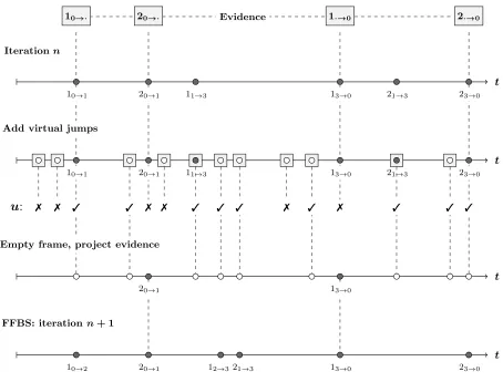
In Figure 5 we observe a task transition diagram with a single iteration in the proposed sampler, for the bottleneck network in Figure 1 (top). In this example, two tasks (num-bered 1 and 2) are observed entering and leaving the net-work at different times; however, there exists no information regarding job services within the network. In each iteration, the sampler begins with a network path whose task tran-sitions are fully compatible with the existing evidence. In an initial step, the existing path is supplemented with vir-tual transitions at the corresponding Poisson rates. In the Figure, we observe that nodes for both virtual jumps and the unobserved job services are superimposed over shaded boxes; the boxes represent further evidence for the lack of task arrivals or departures at these times. Next, auxiliary variables are produced across real and virtual jumps, the subsets are loosely represented by ticks (Γ∪∅) and crosses
({T(x0i−1, x0i)}) for open and clamped nodes respectively. Then, the uniformized frame is emptied and both real and auxiliary evidence is propagated, imposing task transitions
or virtual jumps within clamped nodes and resulting in a restricted frame for possible network paths. Finally, a new compatible path is sampled via forward filtering backward sampling as summarized in Algorithm 2; this will consider the imposed task transitions and weight successive network states over the clamped epochs. The resulting path is fully compatible with the observed evidence, however, notice that task transitions at arrival or departure times may change between iterations.
Note that by choosing Ω strictly greater than all values in the diagonal ofQ, the resulting Markov chain over posterior network transitions is irreducible. Increasing the dominat-ing rate will improve mixdominat-ing in exchange for higher compu-tational requirements. Finally, we note that a high value of pmay hinder the sampler from fully exploring the posterior range of network paths.
3.1.4 Parameter sampling
Finally, given a new family of network realizations X = {Xk}
k=1,...,K fully compatible with observation sequences ˜
O={Ok}k=1,...,K, we may obtain posterior samples of ar-rival and service rate parameters. For traditional FCFS stations this is such that
λc|X ∼Gamma δc,PKk=1Tk and
µci|X ∼Gamma γic, τic
,
forc∈ C, i= 1, . . . , M; assuming independent network pa-rameters and uninformative priors. Here δc, γic andτ
Iterationn
t
10→1 20→1 11→3 13→0 21→3 23→0
Evidence
10→· 20→· 1·→0 2·→0
Add virtual jumps
t
10→1 20→1 11→3 13→0 21→3 23→0
u
:
7 7 3 3 7 7 3 3 3 7 3 7 3 3 3Empty frame, project evidence
t
20→1 13→0
FFBS: iterationn+ 1
t
[image:8.612.79.533.51.396.2]10→2 20→1 12→321→3 13→0 23→0
Figure 5: Task transition diagram with a single iteration in the proposed sampler, for a bottleneck network with three servers. Here, tasks 1 and 2 are observed entering and leaving the network. First, start with a path whose task transitions are fully compatible with the evidence. Then, supplement it with virtual jumps at the corresponding rates, and produce auxiliary variables across real and virtual nodes. Next, empty the uniformized frame and propagate both real and auxiliary evidence; imposing task transitions or virtual jumps within clamped nodes. Finally, repopulate the frame via forward filtering backward sampling, hence maintaining agreement with the existing evidence.
by a class c job, in all realizations in X. Finally, poste-rior probability vectors for class c routings in every node i= 1, . . . , M are given by
Pi,c·|X ∼Dir 1+κci
whereκc
i defines a vector of transition counts from serveri inX. Arrival posteriors inpare defined the same way. We note that in order to ease identifiability in the inferential problem, it is also possible to fix parameters, incorporate conjugate priors or to impose inequality constraints and bounds across parameters; we will show examples in Sec-tion 4 below. Also, the above expressions must be altered when stations respond to prioritization regimes other than FCFS (see Example 3 in Section 4).
4
Examples
In the following, we discuss results obtained across three example networks with both synthetic and real data, in
or-der of increasing difficulty. In all cases, results are obtained through a JAVA implementation of the proposed sampler, and starting compatible network paths have been manually assigned.
The examples demonstrate the ability of the proposed algorithm in order to handle missing data in multi-class inferential problems with varying service disciplines, class switching and imposed prior constraints. Hence, the sam-pler offers the means to overcome necessary assumptions linked to the common use of product form equilibrium pressions for QNs. To the best of our knowledge, there ex-ists no alternative approach overcoming these restrictions when drawing exact inference in general open Markovian networks.
4.1 Tandem network
0 50 100 150 200
0.19500.19750.20000.20250.2050
Service Rate 1
Density
0 10 20 30 40
0.46 0.48 0.50 0.52 0.54
Service Rate 2
Density
0.00 0.25 0.50 0.75 1.00
0 5 10 15 20 25
Lag
A
CF r
ate 1
0.00 0.25 0.50 0.75 1.00
0 5 10 15 20 25
Lag
A
CF r
ate 2 0.48
0.50 0.52
0.194 0.196 0.198 0.200 0.202 0.204
Service rate 1
Ser
vice r
ate 2
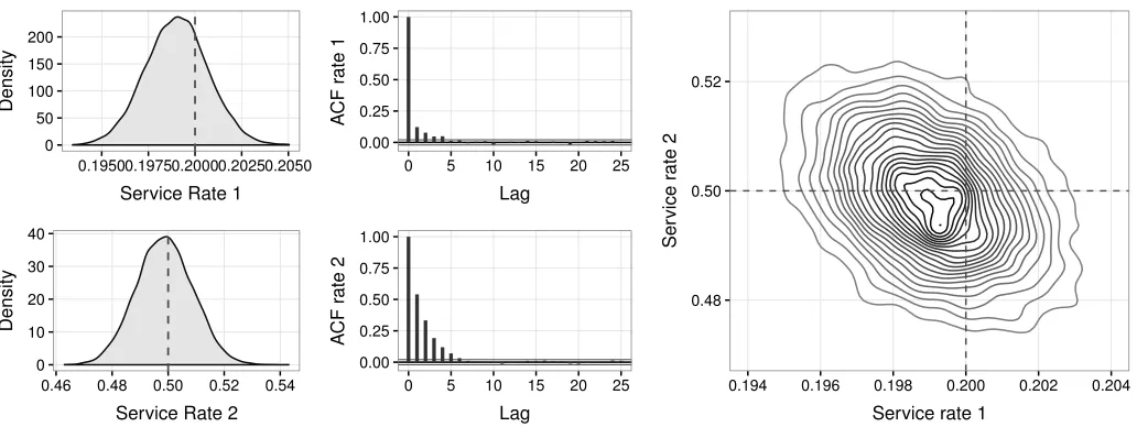
[image:9.612.49.565.71.265.2]Grahical summary of output in tandem network
Figure 6: Graphical summary of output for a single-class tandem network fitted to synthetic data. On the left, we observe the posterior distribution of service rate parameters with original valuesµ1= 0.2 andµ2= 0.5. Black bars in the center correspond to autocorrelation values. On the right, a contour plot for the joint posterior density of rates (dashed lines represent real values).
disciplines and a single task class. Data is generated so that true service rates areµ1 = 0.2 and µ2 = 0.5, arrivals are given byλ= 0.12 and the network topology is defined by a routing probability matrixP such that P1,2 = 1 and P2,0= 1. Also, jobs enter directly into the first queue and p0,1= 1.
For the inferential problem, job service observations (in first station) are always ignored and the only source of in-formation are end-to-end measurements. Thus, available knowledge is limited to the times when tasks enter the queue on the first station and when they depart through the sec-ond station. Overall, we examine 5000 realizations totalling 17827 tasks during 115601 time units. For the purpose, the network topology inP is fixed deterministic, since there ex-ists a unique route from start to completion of tasks. Also, in order to ensure identifiability we impose an inequality constraint on service rates and assign fairly uninformative parameter priors, so that
π(µ1, µ2)∝I(µ1≤µ2)×exp(−10−3(µ1+µ2)).
Note that the problem directly links to the inferential task with two exponentially distributed random variables when only its sum is observed, with the further complexity that unknown waiting times have to be discounted from the em-pirical observations.
In Figure 6 (right) we observe a contour plot for the joint posterior kernel density estimation over service rates, and we notice a significant negative correlation in values (the dashed vertical and horizontal lines represent the orig-inal parameters values in the network path simulations). Results are obtained across two chains with 100000 iter-ations each, a 10000 burn-in stage, varying starting rates
and different scales for dominating rates and probabili-ties producing auxiliary-observations, so that p1 = 0 and Ω1 = 2 maxx∈S|Qx| and p2 = 0.25,Ω2 = 1.5 maxx∈S|Qx|. Note that the second chain is produced employing restric-tive auxiliary-observations as opposed to the first; hence, stronger serial dependencies across subsequent latent paths in the network should be expected. Yet, the remainder plots show marginal posterior kernel density estimations for both service rates, along with an autocorrelation summary across a thinned sample in the second chain, showing a satisfactory mixing.
A discussion on the effects and computational gains re-sulting from employing restrictive auxiliary observations fol-lows in the next example. In general, networks of interest are complex andp= 0 would pose a computationally infea-sible problem. Also, even in simple networks such as this example, computing times can be excessive, and consider-able reductions can be traded at the cost of higher serial dependences.
4.2 Bottleneck network
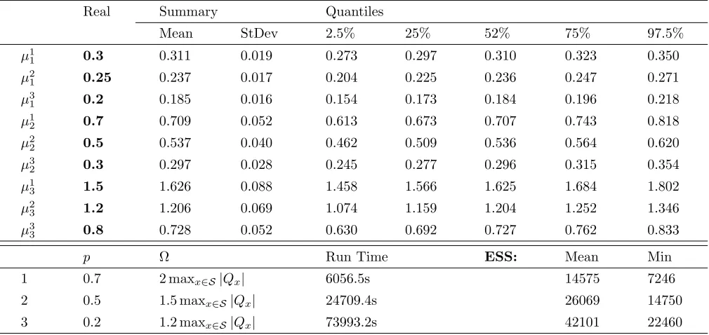
Table 1: Summary statistics for posterior service rates along with computing times across three chains tuned differently in the bottleneck network in Figure 1 (top).
Real Summary Quantiles
Mean StDev 2.5% 25% 52% 75% 97.5%
µ1
1 0.3 0.311 0.019 0.273 0.297 0.310 0.323 0.350
µ21 0.25 0.237 0.017 0.204 0.225 0.236 0.247 0.271
µ3
1 0.2 0.185 0.016 0.154 0.173 0.184 0.196 0.218
µ1
2 0.7 0.709 0.052 0.613 0.673 0.707 0.743 0.818
µ22 0.5 0.537 0.040 0.462 0.509 0.536 0.564 0.620
µ3
2 0.3 0.297 0.028 0.245 0.277 0.296 0.315 0.354
µ1
3 1.5 1.626 0.088 1.458 1.566 1.625 1.684 1.802
µ2
3 1.2 1.206 0.069 1.074 1.159 1.204 1.252 1.346
µ33 0.8 0.728 0.052 0.630 0.692 0.727 0.762 0.833
p Ω Run Time ESS: Mean Min
1 0.7 2 maxx∈S|Qx| 6056.5s 14575 7246
2 0.5 1.5 maxx∈S|Qx| 24709.4s 26069 14750
3 0.2 1.2 maxx∈S|Qx| 73993.2s 42101 22460
defined by{Pc, pc :c∈ C}, where
Pc=
0 1 2 3
1 0 0 0 1
2 0 0 0 1
3 1 0 0 0
,
is identical for all three classes and assumed to be known. In addition, job entries are split evenly, i.e. pc
0,1 = 0.5 and pc
0,2= 0.5 for allc∈ C.
In total, we analyse 500 network realizations totalling 1281 tasks during 5083 time units. In order to ease identifi-ability we assume the existence of a slow, medium and fast server; and assign rather uninformative parameter priors, i.e.
π(µc1,µ c 2, µ
c 3) ∝I(µc1≤µ
c 2≤µ
c
3)×exp(−10
−3(µc 1+µ
c 2+µ
c 3))
for all c ∈ C. Note that this network type may not be analysed by means of product-form representations centred around figures of queue-lengths (c.f Wang et al. (2016)). This is because traditional BCMP networks require FCFS stations to share service rates across task classes. On the other hand, an MCMC sampler as presented in (Sutton and Jordan, 2011) can be extended in order to handle general service distributions and target network path transitions; however, the framework is not designed for such aim, it would require an additional Metropolis-Hastings step and it is likely to perform poorly.
[image:10.612.317.567.378.519.2]In Table 1 we observe summary statistics, computing times and effective sample sizes across three chains with 100000 iterations each, a 10000 burn-in stage, varying start-ing rates and different scales for dominatstart-ing rates Ω and
Table 2: Correlation matrix between service rate parame-ters in a bottleneck network.
µ21 µ31 µ12 µ22 µ32 µ13 µ23 µ33
µ11 -0.02 -0.01 -0.05 0.01 0.01 -0.05 0.01 0.02
µ2
1 -0.02 0.00 -0.03 0.01 0.01 -0.04 0.01 µ3
1 0.01 0.01 -0.09 0.00 -0.01 -0.06
µ1
2 -0.03 -0.05 -0.13 0.01 0.01
µ22 -0.02 0.00 -0.10 0.01
µ3
2 0.00 0.00 -0.10
µ1
3 0.01 0.01
µ23 0.01
4.3 Feedback network
Finally, we show how the proposed sampling scheme may be used to analyse a real data set. For the purpose, we employ work-logs for medical clinicians. Briefly, the data set in-cludes task requests and completions for individual doctors outside the 9:00-17:00 Monday to Fridayin hours settings. It belongs to two jointly coordinated university hospitals in the United Kingdom, together servicing a geographical re-gion with over 2.5 million residents. In Figure 7 we show
t
0 t1 t2 t3 t4 t5 t6 Fall
[image:11.612.54.279.186.269.2]Clerking Urgency
Figure 7: Sample diagram with a subset of tasking data linked to a clinician during a shift
a diagram with a small of subset of data linked to a clini-cian during a shift; there we observe three overlapping tasks recorded in the system (from request to completion), and each belonging to a different class. Note that it is not possi-ble to know when the clinician was engaged with each duty; as individual jobs for tasks are not registered when queueing or being routed across teams of administrative staff, nurses and doctors. An extended description of the data set may be found in Perez et al. (2016).
Multiple tasks are grouped across 14 categories and anal-ysed with afeedback network as shown in Figure 8. There, we notice the presence of two M/M/1 servers with alter-native disciplines and route switching among classes. Task observations for doctors are of roughly two kinds, based on whether they require engagement or not. Many tasks are recorded and erased within doctor work-logs in a short time span, due to no need for action; on the other hand, the re-mainder of tasks exhibit long processing times indicating the need for considerable doctor activity.
P
F CF S
P S
Figure 8: Feedback network with two M/M/1 servers and route switching among task classes.
In the proposed example, arrival jobs are buffered within an administrative FCFS priority type queue and depart to a transition center where they either leave the system or get routed for processing with some unknown probability.
[image:11.612.320.565.262.735.2]Once they are assigned to further processing, they join the doctor’s processing centre and switch their routing mecha-nism; so they will depart the network next time they un-dergo administrative processing in the first queue. The ser-vice station aimed to capture strain on doctor workload is assigned a processor sharing (PS) discipline with a single worker, aiming to accommodate doctors attending concur-rent duties outside standard working hours. No job service observations are available, so thatq= 0 and only the arrival and departure times for tasks to the network are observed. In total, we analyse a reduced subset of 10000 doctor shifts roughly distributed across 4 years of observations.
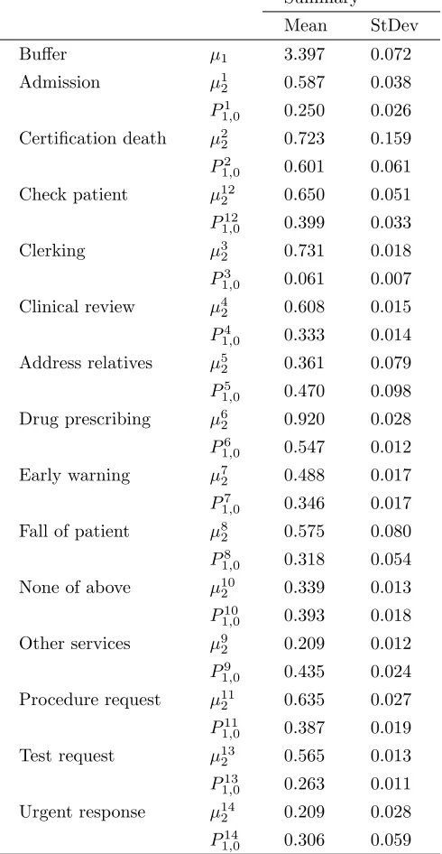
Table 3: Summary statistics for rate and routing parameters in a feedback network.
Summary
Mean StDev
Buffer µ1 3.397 0.072
Admission µ12 0.587 0.038
P1
1,0 0.250 0.026 Certification death µ2
2 0.723 0.159
P2
1,0 0.601 0.061
Check patient µ122 0.650 0.051
P12
1,0 0.399 0.033
Clerking µ3
2 0.731 0.018
P13,0 0.061 0.007
Clinical review µ4
2 0.608 0.015
P4
1,0 0.333 0.014 Address relatives µ52 0.361 0.079
P5
1,0 0.470 0.098 Drug prescribing µ6
2 0.920 0.028
P16,0 0.547 0.012
Early warning µ7
2 0.488 0.017
P7
1,0 0.346 0.017
Fall of patient µ82 0.575 0.080
P8
1,0 0.318 0.054
None of above µ10
2 0.339 0.013
P10
1,0 0.393 0.018
Other services µ92 0.209 0.012
P9
1,0 0.435 0.024 Procedure request µ11
2 0.635 0.027
P111,0 0.387 0.019
Test request µ13
2 0.565 0.013
P13
1,0 0.263 0.011 Urgent response µ142 0.209 0.028
P14
[image:11.612.73.268.554.636.2]The network topology is partially known; i.e. P2c,1=pc0,1= 1 for all task classes, and P1c,0 = 1 after tasks have un-dergone processing and hence switched routing mechanism. However,Pc
1,0= 1−P1c,2needs to be determined for all ex-isting task classes. Processing rates for tasks are assumed equal in the first service station and different in the PS server; we assign no constraints and we impose loosely un-informative priors such that
π(µci)∝exp(−10−3µci)
for alli∈ {1,2}andc∈ C. Also, note that within a PS dis-cipline posterior rates given network realizations are given by
µc|X ∼Gamma γc,PK
k=1
RTk
0 φ k c(t)dt
,
for all c ∈ C, where γc denotes the number of class c jobs served at the station in all realizations inX; and
φkc(t) =
PJ
j=0I(Jobj is classc)·I(aj < t < dj)
PJ
j=0I(aj < t < dj)
,
[image:12.612.46.298.468.607.2]where summations are across all jobs processed in the PS station in realization k, and aj, dj denote the arrival and departure times of the job to the server. In Table 3 we ob-serve summary statistics for parameters across two chains with 100000 iterations each, a 50000 burn-in stage and vary-ing startvary-ing rates. In one chain, we use Ω = 2 maxx∈S|Qx| and p= 0.75; in the second we have Ω = 1.5 maxx∈S|Qx| andp= 0.5.
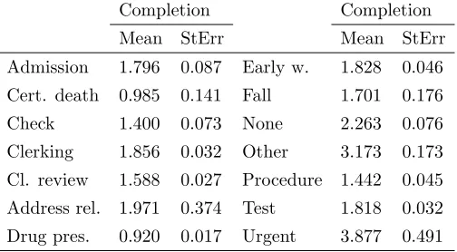
Table 4: Point estimates and standard errors for average processing times excluding waiting times, across different tasks. These relate to times from entry to departure in network.
Completion Completion
Mean StErr Mean StErr
Admission 1.796 0.087 Early w. 1.828 0.046
Cert. death 0.985 0.141 Fall 1.701 0.176
Check 1.400 0.073 None 2.263 0.076
Clerking 1.856 0.032 Other 3.173 0.173
Cl. review 1.588 0.027 Procedure 1.442 0.045
Address rel. 1.971 0.374 Test 1.818 0.032
Drug pres. 0.920 0.017 Urgent 3.877 0.491
In addition, Table 4 shows point estimates and standard errors for average completion times in all task types, these correspond to the full processing times from entry to de-parture in the network (excluding queueing times) and are reported in hour units. Hence, we notice it is possible to assess workload both globally and across single components in the system, thus allowing to answer extrapolation kinds of questions on workload; i.e. in relation to means, vari-ances and extreme values for system strain under likely al-terations.
5
Discussion
This paper has presented a flexible approach for carrying ex-act Bayesian inference within known or hypothesized queue-ing networks. Its focus is on multi-class, open and Marko-vian cases and the approach is centred around the underly-ing continuous-time Markov chains induced by these com-plex stochastic systems. The proposed method relies on a slice sampling technique with mappings to the space of task transitions across servers in the network. It sits well over uniformization-oriented MCMC approaches introduced in Rao and Teh (2013) and can deal with missing data, imposed prior knowledge and strong serial dependencies posing a complex inferential task (cf. Sutton and Jordan (2011)).
The need for such inferential frameworks with missing data is justified by the ability of general-form networks to allow evaluating response times in complex systems. Over-all, recovering measures such as processing times is a techni-cally difficult task when designing increasingly complex IT systems (Liu et al., 2006), or in service delivery networks (such as those in hospitals) due to ethical issues with such an intrusive process (Perez et al., 2016). Yet, QNs provide the tools to assess system alterations, diagnose poor perfor-mance or evaluate robustness to spikes in workload.
The advantage of the presented inferential method is that it permits retrospectively assessing the likely status of systems at any point in time; rather than only provid-ing summary information on strain over individual bits. However, limitations relate to tractability restrictions with high-magnitude networks. In such cases, controlling the dimensionality of unobservable state spaces requires impos-ing strong serial dependencies within simulated latent net-work paths across steps in the sampler. This however may restrict the produced chain from exploring the posterior range of network paths efficiently. Approximate inferential frameworks relying on reduced product-form simplifications of state beliefs may improve the scalability of the method. Moreover, it is possible to explore the use of particle filtering approaches along with auxiliary variables for this purpose, since clamping explorable spaces within filtering procedures would likely ease the usual challenges regarding particle de-generacy; that is, ending with a very few particles having non-zero weights.
Also, the use of the uniformization technique will limit applications of the present framework to the study of purely Markovian processes. While it is possible to em-ploy Markov-modulated regimes that adapt service and ar-rival rates to network states, this will greatly expand state spaces under consideration. Also, uniformization may deem the sampler computationally inefficient should service rates vary greatly across queues or job classes, as certain tran-sition types will greatly dominate the underlying discrete time Markov chain.
For simplicity, q is assumed fixed and known to the user. Many network structures (such as bottleneck networks) will allow for uncertainty regarding this parameter to be quanti-fied by means of the presented sampler, as each iteration will provide a total number of network transitions complement-ing the observation number as a sufficient statistic. How-ever, it is necessary to impose the knowledge of qin order to ensure model identifiability whenever networks contain either global or self-loops.
Supplementary material
Synthetic data along with a Java implementation of the algorithm can be found in https://bitbucket.org/ ikertxo1986/auxvarsamplerjava or https://github. com/IkerPerez/auxVarSampler. This allows to reproduce the results within the examples above.
Acknowledgements
We would like to thank the anonymous reviewers for their valuable remarks and suggestions that have improved the quality of this paper.
References
Armero, C. and Bayarri, M. J. (1994). Prior assessments for prediction in queues.The Statistician, 43(1):139–153.
Baskett, F., Chandy, K. M., Muntz, R. R., and Palacios, F. G. (1975). Open, closed, and mixed networks of queues with different classes of customers. Journal of the ACM, 22(2):248–260.
Boyen, X. and Koller, D. (1998). Tractable inference for complex stochastic processes. InProceedings of the Four-teenth Conference on Uncertainty in Artificial Intelli-gence, UAI’98, pages 33–42.
Buzacott, J. A. and Shanthikumar, J. G. (1993). Stochas-tic models of manufacturing systems, volume 4. Prentice Hall, New Yersey.
Fan, Y. and Shelton, C. R. (2008). Sampling for approxi-mate inference in continuous time bayesian networks. In
Tenth International Symposium on Artificial Intelligence and Mathematics, ISAIM’08.
Hobolth, A. and Stone, E. A. (2009). Simulation from endpoint-conditioned, continuous-time markov chains on a finite state space, with applications to molecular evolu-tion. The Annals of Applied Statistics, 3(3):1204–1231.
Jensen, A. (1953). Markoff chains as an aid in the study of Markoff processes. Scandinavian Actuarial Journal, 36:87–91.
Kalli, M., Griffin, J. E., and Walker, S. G. (2011). Slice sampling mixture models. Statistics and Computing, 21(1):93–105.
Kleinrock, L. (1976). Queueing Systems Vol II: Computer Applications. Wiley, New York.
Koole, G. and Mandelbaum, A. (2002). Queueing models of call centers: An introduction. Annals of Operations Research, 113(1):41–59.
Lippman, S. A. (1975). Applying a new device in the op-timization of exponential queuing systems. Operations Research, 23(4):687–710.
Liu, Z., Wynter, L., Xia, C. H., and Zhang, F. (2006). Pa-rameter inference of queueing models for IT systems us-ing end-to-end measurements. Performance Evaluation, 63(1):36 – 60.
Neal, R. M. (2003). Slice sampling.The Annals of Statistics, 31(3):705–767.
Ng, B., Peshkin, L., and Pfeffer, A. (2002). Factored particles for scalable monitoring. In Proceedings of the Eighteenth Conference on Uncertainty in Artificial Intel-ligence, UAI’02, pages 370–377.
Nodelman, U., Shelton, C. R., and Koller, D. (2002). Con-tinuous time bayesian networks. In Proceedings of the Eighteenth Conference on Uncertainty in Artificial Intel-ligence, UAI’02, pages 378–387.
Osorio, C. and Bierlaire, M. (2009). An analytic finite ca-pacity queueing network model capturing the propaga-tion of congespropaga-tion and blocking. European Journal of Operational Research, 196(3):996 – 1007.
Perez, I., Brown, M., Pinchin, J., Martindale, S., Sharples, S., Shaw, D., and Blakey, J. (2016). Out of hours work-load management: Bayesian inference for decision sup-port in secondary care.Artificial Intelligence in Medicine, 73:34 – 44.
Rao, V. A. and Teh, Y. W. (2013). Fast MCMC sampling for Markov jump processes and extensions. Journal of Machine Learning Research, 14:3295–3320.
Spinner, S., Casale, G., Brosig, F., and Kounev, S. (2015). Evaluating approaches to resource demand estimation.
Performance Evaluation, 92:51 – 71.
Sutton, C. and Jordan, M. I. (2011). Bayesian inference for queueing networks and modeling of internet services.The Annals of Applied Statistics, 5(1):254–282.
Walker, S. G. (2007). Sampling the dirichlet mixture model with slices. Communications in Statistics - Simulation and Computation, 36(1):45–54.
Wang, W., Casale, G., and Sutton, C. (2016). A bayesian approach to parameter inference in queueing networks.