Approximate dynamic programming with combined policy functions for solving multi stage nurse rostering problem

Approximate Dynamic Programming With

Combined Policy Functions for Solving

Multi-Stage Nurse Rostering Problem

Peng Shi and Dario Landa-Silva

School of Computer Science, ASAP Research Group The University of Nottingham, United Kingdom

{peng.shi, dario.landasilva}@nottingham.ac.uk

Abstract. An approximate dynamic programming that incorporates a combined policy, value function approximation and lookahead policy, is proposed. The algorithm is validated by applying it to solve a set of instances of the nurse rostering problem tackled as a multi-stage prob-lem. In each stage of the problem, a weekly roster is constructed taking into consideration historical information about the nurse rosters in the previous week and assuming the future demand for the following weeks as unknown. The proposed method consists of three phases. First, a pre-process phase generates a set of valid shift patterns. Next, a local phase solves the weekly optimization problem using value function ap-proximation policy. Finally, the global phase uses lookahead policy to evaluate the weekly rosters within a lookahead period. Experiments are conducted using instances from the Second International Nurse Roster-ing Competition and results indicate that the method is able to solve large instances of the problem which was not possible with a previous version of approximate dynamic programming.

Keywords: Dynamic Programming, Approximation Function, Policy Function, Nurse Scheduling Problem

1

Introduction

The Nurse Rostering Problem (NRP) is an NP-Hard problem that consists in constructing rosters for a number of nurses over a time horizon of typically no more than a few weeks. Constructing a roster involves assigning shifts types of each nurse for each day in order to fulfill daily duty requirements plus satisfying a number of soft and hard constraints [3]. In this paper, the NRP is tackled as a multi-stage optimisation problem is used to test the proposed technique because it is a widely investigated problem and presents an interesting challenge to ADP. Tackling the NRP as a multi-stage problem was proposed by [4].

Solving the NRP with dynamic programming is impractical due to the curse of dimensionality [2, 5]. Our previous work investigated ADP to solve NRP, where a value function approximation based method was proposed to tackle various in-stances of the NRP [6]. However, the computation time required for constructing solution samples and the memory space required for recording rewards increased exponentially for larger problem instances. Hence, that shortfall has motivated the present work. A number of ADP practical issues related to the complexity of the environment, in particular when dealing with large state or action space, are reported in the literature [5]. The technique proposed in this paper enhances the ability of ADP to solve NRP as a multi-stage problem by combining two policy functions, value function approximation to solve the weekly problem, and lookahead policy to evaluate weekly rosters with artificially constructed future demand within a given lookahead period.

The contribution of this paper is an enhanced approximate dynamic program-ming approach that takes advantage of tackling the NRP in multiple stages and is able to tackle instances of this problem with longer planning horizons. The rest of paper is structured as follows. Section 2 describes NRP used in this inves-tigation and its modelling as a Markov Decision Process. Section 3 explains the details of the proposed algorithm. Section 4 presents the experimental results. Section 5 concludes the paper and outlines future work.

2

The Multi-Stage Nurse Rostering Problem

In the multi-stage nurse rostering problem the planning horizon is seen as mul-tiple non-overlapping stages, nurse rosters should be selected one stage at a time. A stage is a part of the planning period for which the demands are com-pletely known at its start [7]. In this paper, the Second International Nurse Rostering Competition (INRC-II) instances are used for experimentation. In these instances, each stage is a week under the competition setting. This section outlines the problem and its modelling as a Markov Decision Process proposed in a previous paper [6].

2.1 Problem Description

H1 A nurse can be assigned at most one working shift per day.

H3 Two consecutive shifts of a nurse must follow a legal shift type successor, for example a late shift could not be followed by a early shift.

H4 A shift of a given skill must be fulfilled by a nurse having that skill. S5 Each nurse is required to either work or rest on both days of weekends. S6 For the whole planning period, each nurse has a minimum and maximum

total number of working assignments.

S7 For the whole planning period, each nurse works a maximum number of weekends.

Week requirement is a list of specific hard or soft constraints in each week:

H2 For each day, shift or skill combination, the assigned number of nurses must cover the minimum requirement.

S1 The number of nurses for each shift with each skill must be equal to the optimal requirement.

S2 Maximum and minimum number of consecutive assignment per shift or day. S3 Maximum and minimum number of consecutive days off.

S4 Respect to the specific shift requirement for each nurse.

History data is a summary of the acutal roster for the previous stage which is required when tackling the problem. If the first week is the current solving stage, history data is randomly selected from built-in artificial files [4]. History data for each stage must be produced by solvers before processing to the next stage and it should include the following information for each individual roster:

• the last assignment of previous week.

• consecutive assignments of the same type as last day.

• total number of worked shifts.

• total number of worked weekends.

In the above list of constraints, H indicates hard constraints that must be satisfied by a solution to be considered feasible andS indicates soft constraints that incur a penalty if violated.

2.2 Problem Modification

Given that in each stage the future demand in this multi-stage NRP is considered as unknown, we apply the framework by Powell [2] which considers the exogenous information. The Markov Decision Process (MDP) notation is summarized as

{S, A, W, T r(S, A, W)}.

Sis astatevariable, split as pre-decision state and post-decision state. The pre-decision state is the start point and the post-decision state is a termination for each stage. For each stage t in the NRP, the pre-decision state variable corresponds to the combination of weekly schedules from stages 1 tot−1, and

Ais anactionvariable which determines the policy selected in the current stage. In the NRP,Ais a weekly roster where each nurse is assigned a combina-tion of integer variables indicating the shift type for each day. The feasibility of a solution is controlled by the selection of decisions.

W is defined asexogenous informationwhich is available only within each stage t. In the NRP,W represents the weekly requirements (local constraints) described above.

Thetransition functionT r(S, A, W) transfers a pre-decision state to the post-decision state with the decision A and the exogenous information W. In the NRP considered here, the transition function performs two roles, one is to update the solution with weekly roster A and week dataW and the other one is to update the nurse historical information based on the value of AandW.

3

Proposed Algorithm

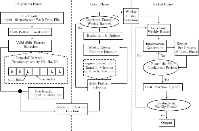
The structure of the proposed algorithm is exhibited in figure 1 and consists of three parts. First, the pre-process phase sets up the search space. Then, the local phase is an enhancement of our previous work [6] for solving the weekly optimization problems. Finally, the global phase applies a lookahead policy for future demand evaluation. Each of these parts is explained below.

Shift Pattern Constructor

Valid Shift Pattern

Length:7 (a week) Feasibility: satisfy H1, H3, H4

File Reader

File Reader

Local Phase Global Phase

b

Nurse Shift Pattern Detection

Shift Pattern Selection e-greedy selection: Random Selection or Greedy Selection

Combine Function Evaluation & Update

Weekly Selection Roster No Yes Information Generation Select one Weekly Roster Pre-process Phase Repeat Pre Process & Local Phase

Cost Function Update

Output Yes No

Yes

E E L L L

day index shift index

input: Scenario and Week Data File

input: History File

Selection Weekly Roster

Construct Enough Weekly Roster?

Reach the Max Lookahead Period?

No

Evaluate All Weekly Roster?

3.1 Pre-process Phase

If a shift pattern (SP) is defined as a weekly roster of a nurse, then a solu-tion should be described as the combinasolu-tion of nurses’ shift patterns. A solusolu-tion is feasible if and only if each constructed SP satisfies all the hard constraints. Exploring infeasible solutions is not required in the principle-of-optimality ap-proaches [2]. Instead, evaluating feasible-shift-pattern based solutions has the potential to make the search more efficient. With this purpose, the pre-process phase is designed to construct a reduced search space for the subsequent local and global phases.

The pseudocode of this pre-process phase is shown in algorithm 1. Hard constraints selected to filter shift patterns belong to global information (2.1) which each individual nurse roster is expected to obey. The set that contains all feasible shift patterns is defined as feasible set. Lines 2-6 are the selection steps, wheresp indicates a single shift pattern andvsp represents the feasible set.

Once the feasible set is prepared, some shift patterns are not available to specific nurses with the consideration of nurse history data. For example, if the last assignment of a nurse in history data is a late shift, then any pattern starting with an early shift in the feasible set becomes infeasible for this nurse (2.1H3). Lines 7-13 represent the specific shift pattern selection procedure of each nurse with the consideration of related history data.

Algorithm 1Pre-process Phase

1: vsp←null; 2: repeat

3: sp←Shif tP atternConstructor(); 4: if spsatisfy hard constraintsthen

5: addsptovsp;

6: untilno more action from constructor

7: forEach Nursendo

8: ivsp←null;

9: Collect the last assigned shift typexlast;

10: foreach sp∈vsp do

11: Selectx1 fromsp;

12: if {xlast, x1}satisfy hard constraintthen

13: addsptoivsp

3.2 Local Phase - Value Function Approximation

guaranteed to be the one incorporated into the overall solution. Therefore, the output of this local phase is a selection of weekly rosters as depicted in figure 1.

Q(S, a) =r(S, a) +γmaxa0Q(δ(S, a), a0) (1)

The Q-learning function, presented in Eq (1), is applied to tackle the local phase problem. The aim is to update the value ofS when changes are made by the selecteda. In this multi-stage nurse rostering problem,S is a weekly roster and a is a list of selected shift patterns for nurses. Shift patterns are selected based on two methods.Random Selection is applied ifSis not fully constructed or sample size of S is small. Shift patterns of unassigned nurses in the roster will be randomly selected. This selection is replaced by Greedy Selection after constructing a number ofS. For a fully constructedS, shift pattern of one or a list of nurses is updated by the one with minimum cost, or equally described as highest reward, from previous steps.r(S, a) is the reward function and calculated from two aspects, the overall constraint violation update and times of the selected

a. The pseudocode of this local phase is shown in algorithm 2.

Algorithm 2Local Phase - Value Function Approximation

1: Initial value ofmax iter,

2: i←0,M ←Empty SList←Empty;

3: whilei < max iterdo

4: Sol←Empty

5: forEach Nursendo

6: rnd←RandomN umberGenerator() 7: if rnd < then

8: sp←RandomSelection(ivsp)

9: else

10: sp←GreedySelection(ivsp) 11: Insert(Sol, sp)

12: c=CostF unction(sp) 13: U pdateV alue(V(Sol), c) 14: Add(SList, Sol)

15: e=ExpectedF unction(SList)

16: γ=P arameter(V(Sol), e) 17: U pdateV alue(V(Sol), γ×e) 18: U pdate()

19: i←i+ 1

20: W eeklyRosterSelection(SList, M)

with a degree of variety and not only concentrating on the local optimum. The selected shift pattern sp is added to Sol in line 11. In line 12, CostFunction calculates the shift pattern cost (c) according to the violation of soft constraints S1-S5and then the value of this weekly roster is updated in line 13.

In line 14, the fully constructed weekly rosterSolis stored in the sample list

SList. Lines 15-18 correspond to theEvaluation & Update in figure 1. The

pur-pose of the expected function is to indicate the average value of the constructed weekly roster while γ is an importance factor and its value is adjusted in the opposite direction to the value of the constructed weekly roster. For instance, if the cost value of a particular weekly roster is larger than the expected value, the value ofγis set to a smaller value, and vice verse.

The end of this local phase in line 20 results in the output setM which is a subset ofSList, i.e. a set of weekly rosters some with small constraint violation

cost (due to the greedy selection) and others with possibly large cost (due to the random selection). This setM is the input to the global phase described in the following subsection.

3.3 Global Phase - Lookahead Policy

In the local phase, the weekly rosters are evaluated for the weekly constraints only, i.e. from H1 toH4 and fromS1 to S5. However, since in each week the future demand is unknown, the global constraintsS6andS7are not considered. Then, this global phase evaluates the weekly rosters with artificial future demand through a lookahead period. The lookahead policy seeks to construct a potential solution within a lookahead period based on the weekly roster and artificial future demand in order to evaluate the solution for the global constraints. The input to this global phase is the set of weekly rostersMfrom the local phase. The output is one weekly roster only as the final solution to the weekly optimization problem. The pseudocode of the global phase is shown in algorithm 3 which is applied to each weekly roster inM. The methodInformation Generationwill be explained in section 4, here we assume all the artificial future demand is obtained in advance.

LK(S) is the lookahead value for each weekly rosterS and calculated using equation 2. n is the nurse index. stage is the week index. T is the lookahead period. spn is a single shift pattern of nursen in the weekly roster S. xnt is a

shift pattern at the lookahead staget of nurse n.xnt belongs to the valid shift

pattern setV SPnt.

LK(S) =

N X

n=1

T+stage X

t=stage

minnV(spn, xnt) (2)

This global phase incorporates the pre-process and local phases described above. For each nursen, the valid shift pattern setV SPntis constructed in line

7 based on the current shift pattern spn and the artificial weekly demand at

lookahead period t. We select the shift pattern xnt in V SPnt with the lowest

Algorithm 3Global Phase

1: Initial value ofLK(S);

2: forEach Nursendo

3: selectspn fromS

4: Initialideal sol=Insert(spn, φ)

5: V(ideal sol) =V(spn)

6: fort←stage to T +stagedo

7: V SPnt←P re−processP hase

8: xnt←GreedySelection(V SP)

9: c←CostF unction(xnt)

10: U pdateV alue(V(ideal sol), c) 11: Insert(ideal sol, xnt)

12: c←CostF unction(ideal sol) 13: U pdateV alue(V(ideal sol), c) 14: U pdateV alue(LK(S), V(ideal sol))

and xnt in lines 8 and 11. The initial value of this ideal solution is the same

value ofspn and is updated with the constraint violation cost ofxnt in line 10.

Lines 7-11 are repeated until reaching the last lookahead stage T+stage. The value of ideal solis then added the constraint violation of S6 andS7. This is the evaluation of a single shift patternspn and this value is added toLK(S) for

each nursen.

Once all the weekly rosters are evaluated through the algorithm 3, the one with lowest LK(S) will be selected as the final weekly solution and the nurse historical information is updated for the following week.

4

Experimental Design and Results Analysis

The problem instances for evaluating the proposed approach are selected from the Second International Nurse Rostering Competition (INRC-II) [4]. The are three sets of instances, all available at [8]. One is a test set with small number (up to 21) of nurses. Another is the competition set released to the competitors. The last set is a hidden set that was made available at the end of the competition. For the experiments here we use the first two data set only.

The proposed algorithm described in section 3 was implemented in Java (JDK 1.7) and all computations were performed on an Intel (R) Core (TM) i7 CPU with 3.2 GHz and RAM 6 GB.

4.1 Experimental Settings

For a problem that considers 3 working shifts and 1 day off per day of the week, the total number of possible shift patterns is 16384 (47_{). The pre-process phase}

model. As the search space is considerably small after the pre-process phase, we implement a lookup table in the local phase procedure.

The initial value of is set to 0.9 and is updated based on the Generalized Harmonic Step Size Function [2]. Through preliminary experimentation we tuned the size of the simulation sample SList = 100 and the output set M = 30 in

the local phase. Also through preliminary experiments and results analysis, we decided to select elements from SList for M following the 1-6-3 rule. That is,

10% is selected from S List with the lowest V(S), the 90% of S List is split into two subgroups, good and bad, based on the constraint violation cost. Then 60% is randomly selected from the good subgroup and 30% is randomly selected from the bad subgroup.

The cost value for both single shift pattern sp and weekly rosterS is cal-culated using Eq. (3) where cs is the soft constraint violation cost and Vsc is

the number of violation for each constraint. The calculation of the constraint violation is fully described in [4].

c= X

eachconstraint

cs×Vsc (3)

The artificial future demand is generated by randomly selecting a week data file per week in the lookahead period. Back to the algorithm described in the section 3, only one future path is evaluated for each weekly roster. Less evaluations of lookahead policy is not ideal but more evaluations consume much computation time and memory. By preliminary experiments we found that 1000 evaluations is the minimum to achieve the level of performance in our results while still using considerably short computation time. The value ofLK(S) is updated based on Eq. (4). All experimental results presented in the rest of this section correspond to 20 runs for each problem instance.

LK(S) = 1

k

k X

i=1

LKi(S) (4)

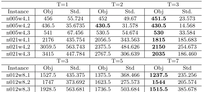
4.2 Lookahead Period Comparison

We tested various lookahead periods for each planning horizon. The lookahead period T for scenarios with 4 weeks is set as 1, 2 and 3 and as 3, 5 and 7 for scenarios with 8 weeks. All the scenarios from the test set were used for these experiments comparing the different values of T and results are presented in table 1.

T=1 T=2 T=3

Instance Obj Std. Obj Std. Obj Std.

n005w4 1 456 55.724 452 49.67 451.5 23.573

n005w4 2 436.5 35.6735 430.5 31.578 430.5 14.568

n005w4 3 541 67.456 530.5 54.674 530 33.584

n021w4 1 2176 435.754 2056.5 343.563 1815 185.683

n021w4 2 3059.5 563.743 2375.5 484.626 2150 254.673

n021w4 3 3415 447.784 2767.5 306.639 2035 186.460

T=3 T=5 T=7

Instance Obj Std. Obj Std Obj Std

n012w8 1 1527.5 435.375 1375.5 368.466 1237.5 235.256

n012w8 2 1747 373.692 1623.5 275.573 1544 205.574

n012w8 3 1928.5 563.681 1736.5 503.684 1515.5 385.678

Table 1.The Average Objective Value and Standard Deviation Obtained with Various Lookahead Periods for Each Instance. Best values are indicated in bold.

4.3 Algorithm Validation and Comparison

Based on the observations from the experiments with the test set, the lookahead period was set toT = 3 for 4-week instances and toT = 7 for 8-week instances on experiments with the competition data set. Results are presented in table 2. A value of99999 in the table indicates that the approach ran out of memory. The performance of the proposed ADP-CP is evaluated through two aspects for each instance. In the left part of the table 2 we compare it with each individual policy. The solution constructed by individual simulation approach is a combina-tion of optimal weekly rosters. The global constraints are considered only when solving the weekly optimization problem in the last stage. On the other hand, the individual lookahead policy focuses on the solution evaluation of global con-straints but each weekly solution is solved with random selection approaches. Looking further has the benefit on the overall solution by comparing the value in columns 2 and 4. Local optimum is only concentrated on the assignment pat-terns, such as the consecutive working patterns and the consecutive days off. We select the instancen030w4 1 as an example. The number of working shifts for each nurse is set as 4 to avoid local constraint violations. The total working days for each nurse is 16 in the final solution. However in some contract, the minimum total working days is 20. A significant large global constraint violation cost is added to the final objective value. A good weekly roster also improves the optimality of lookahead policy with the comparison of columns 3 and 4.

program-Instance Simulation Lookahead ADP-CP Best Worst

n030w4 1 1925 2725 1780 1745 9850

n030w4 2 2650 2710 1610 1935 10605

n030w8 1 5350 6645 4830 2295 21185

n030w8 2 6310 5820 4855 1900 21145

n040w4 1 8120 3945 3270 1765 14680

n040w4 2 6895 4260 3735 1910 14460

n040w8 1 14720 10125 9305 3105 35010

n040w8 2 19255 10165 8975 2975 33000

n050w4 1 5900 4070 3535 1525 17745

n050w4 2 6210 4070 3030 1480 15380

n050w8 1 19525 10045 8965 5560 43040

n050w8 2 13905 9725 8420 5475 42765

n060w4 1 18480 16977 12282 2830 19230

n060w4 2 20945 17794 15019 2950 20400

n060w8 1 20215 9590 9720 2840 44130

n060w8 2 17545 11000 10160 3200 44430

n080w4 1 23195 21870 18350 3474 26935

n080w4 2 26305 21435 16885 3535 27210

n080w8 1 48505 44880 35975 4845 64915

n080w8 2 47355 44065 38800 5105 66515

n100w4 1 19625 19295 16045 1445 33740

n100w4 2 20530 20270 17885 2070 33465

n100w8 1 53155 39550 35690 3095 85260

n100w8 2 50340 40755 35440 3135 87445

n120w4 1 99999 24075 22960 2470 36235

n120w4 2 99999 22680 22065 2530 36320

n120w8 1 99999 43215 39170 3555 83590

n120w8 2 99999 40840 41350 3435 82145

Table 2.Experimental Results of the Proposed ADP with Combined Policy (ADP-CP), Individual Simulation Approach, Individual Lookahead Policy, Best and the Worst Results from the Competition. Best values are indicated in bold.

ming, with the approximation policies, for solving this complicated multi-stage nurse rostering problem. This is an important step towards making dynamic programming practical in its application for solving difficult combinatorial opti-mization problems when a multi-stage solving approach can be followed.

5

Conclusion

generate a set of weekly rosters. The third phase is a global phase that imple-ments a lookahead policy to evaluate the effect of the future uncertainty within a lookahead period. The proposed ADP then combines value function approx-imation and lookahead policy. The instances from the Second Nurse Rostering Competition (INRC-II) are used in the experiments to validate the performance of this proposed algorithm. Experimental results show that the combined policy approach in the proposed algorithm produces better performance than the in-dividual policies. Besides, the results obtained with the proposed algorithm on some of the INRC-II problem instances are close to the best solutions reported for the competition. Future works should be focused on improving the solution qual-ity and reducing the computational time. These improvements could be achieved by applying different methods to evaluate the lookahead samples. Furthermore, improving the quality of weekly rosters could also benefit the lookahead policy as arguably better weekly rosters could help to achieve better results with shorter lookahead periods and also reduce the computation time.

References

1. Martin L Puterman. Markov decision processes: discrete stochastic dynamic

pro-gramming. John Wiley & Sons, 2014.

2. Warren B Powell. Approximate Dynamic Programming: Solving the curses of

di-mensionality, volume 703. John Wiley & Sons, 2007.

3. Edmund K Burke, Patrick De Causmaecker, Greet Vanden Berghe, and Hendrik Van Landeghem. The state of the art of nurse rostering. Journal of scheduling, 7(6):441–499, 2004.

4. Sara Ceschia, Nguyen Thi Thanh Dang, Patrick De Causmaecker, Stefaan Haspes-lagh, and Andrea Schaerf. Second international nurse rostering competition (inrc-ii)—problem description and rules—. arXiv preprint arXiv:1501.04177, 2015. 5. Gerald Tesauro. Practical issues in temporal difference learning. InReinforcement

Learning, pages 33–53. Springer, 1992.

6. Peng Shi and Dario Landa-Silva. Dynamic programming with approximation func-tion for nurse scheduling. In International Workshop on Machine Learning,

Opti-mization and Big Data, pages 269–280. Springer, 2016.

7. Nguyen Thi Thanh Dang, Sara Ceschia, Andrea Schaerf, Patrick De Causmaecker, and Stefaan Haspeslagh. Solving the multi-stage nurse rostering problem. In Pro-ceedings of the 11th International Conference of the Practice and Theory of

Auto-mated Timetabling, pages 473–475, 2016.