1 Quantification of root water uptake in soil using X-ray Computed Tomography and 1
image based modelling. 2
3
Author list: Keith R. Daly$§1, Saoirse R. Tracy$2, Neil M. J. Crout3, Stefan Mairhofer4, Tony 4
P. Pridmore4, Sacha J. Mooney3 and Tiina Roose1 5
6
Author affiliations: 7
1
Bioengineering Sciences Research Group, Faculty of Engineering and Environment, 8
University of Southampton, University Road, Southampton, SO17 1BJ, United Kingdom, 9
2
School of Agriculture and Food Science, University College Dublin, Belfield Campus, 10
Dublin 4, Ireland. 11
3
School of Biosciences, University of Nottingham, Sutton Bonington Campus, 12
Leicestershire, LE12 5RD, United Kingdom. 13
4
School of Computer Science, University of Nottingham, Jubilee Campus, Nottingham, NG8 14
1BB, United Kingdom. 15
16
$
These authors are joint lead authors 17
§
Corresponding author: email: [email protected] 18
19
2 1. Abstract
21 22
Spatially averaged models of root-soil interactions are often used to calculate plant water 23
uptake. Using a combination of X-ray Computed Tomography (CT) and image based 24
modelling we tested the accuracy of this spatial averaging by directly calculating plant water 25
uptake for young wheat plants in two soil types. The root system was imaged using X-ray 26
CT at 2, 4, 6, 8 and 12 days after transplanting. The roots were segmented using semi-27
automated root tracking for speed and reproducibility. The segmented geometries were 28
converted to a mesh suitable for the numerical solution of Richards’ equation. Richards’ 29
equation was parameterised using existing pore scale studies of soil hydraulic properties in 30
the rhizosphere of wheat plants. Image based modelling allows the spatial distribution of 31
water around the root to be visualised and the fluxes into the root to be calculated. By 32
comparing the results obtained through image based modelling to spatially averaged models, 33
the impact of root architecture and geometry in water uptake was quantified. We observed 34
that the spatially averaged models performed well in comparison to the image based models 35
with <2% difference in uptake. However, the spatial averaging loses important information 36
regarding the spatial distribution of water near the root system. 37
38
Keywords: Matric potential; rhizosphere; root water uptake; soil pores; wheat; water release 39
characteristic; X-ray Computed Tomography; image based homogenisation. 40
41
Abbreviations: 42
(CT) – Computed Tomography 43
3 Short title for page headings: Quantification of root water uptake in soil
45 46
2. Introduction 47
The fundamentals of plant water uptake, in particular the influence of the geometry of micro-48
scale root-soil interactions, are not fully understood. Further knowledge surrounding the 49
mechanisms behind water flow in soil and into roots is crucial for modelling root water 50
uptake. As plants grow they alter the soil immediately adjacent to the root creating a region 51
known as the rhizosphere (Hiltner, 1904) through a combination of mechanical compression 52
of the soil (Dexter, 1987; Whalley et al., 2013; Whalley et al., 2005), creation of biopores 53
(Stirzaker et al., 1996) and exudation of chemical compounds such as mucilage (Czarnes et 54
al., 2000) which, in turn, enhances microbial growth (Gregory, 2006). The role of the 55
rhizosphere in terms of water retention and uptake has been the subject of a great number of 56
studies . In dry conditions it is found that the rhizosphere is wetter than the surrounding soil, 57
whilst in wet conditions the rhizosphere is drier than the surrounding soil (Carminati, 2012; 58
Moradi et al., 2011). Other studies suggest rhizosphere soil may be wetter than bulk soil 59
(Young, 1995) due to the formation of a coherent sheath of soil permeated by mucilage and 60
root hairs, known as the rhizosheath (Gregory, 2006). Small quantities of water are released 61
from the root to the rhizosheath at night while the root absorbs water from the rhizosheath 62
during the day (Walker et al., 2003). The soil around a root and the processes that take place 63
to form the rhizosphere soil clearly have a significant influence on root water uptake. 64
However, currently we cannot mechanistically predict the role that root geometry plays in 65
water uptake. This is due to the difficulties associated with imaging and quantifying roots, 66
soil, and water simultaneously for growing root systems. 67
4 In order to improve understanding and provide a detailed description of water movement in 69
and around the rhizosphere, research has generally focused on a combination of imaging and 70
image based modelling studies (Daly et al., 2015). It is possible to use X-ray CT to quantify 71
soil structure, water and air filled pore space (Rogasik et al., 1999) and, from the images 72
generated, model partially saturated hydraulic conductivity in bulk soil (Tracy et al., 2015). 73
Recently 3-dimensional (3D) segmented root architectures of faba bean (Vicia faba L.) have 74
been used in a root-soil water movement model to determine the hydrodynamics of root water 75
uptake in a split pot system (Koebernick et al., 2015). At the plant root scale, it is not 76
computationally feasible to resolve the pore geometry in detail and averaged models for flow 77
and transport are often used (Hornung, 1997; Keller, 1980; Richards, 1931). Formally, these 78
models can be derived from the underlying pore scale models using mathematical techniques 79
such as homogenisation (Cioranescu and Donato, 1999; Pavliotis and Stuart, 2008). 80
Homogenisation methods are based around the idea that the behaviour of a system can be 81
calculated by solving underlying equations on a representative region of soil. From a 82
physical point of view, this method provides averaged equations and the means to derive the 83
value of physical constants on which these equations depend based on the observed X-ray CT 84
images. These methods are well suited to flow problems in soil and have been developed for 85
single porosity materials (Hornung, 1997; Keller, 1980), double porosity materials (Arbogast 86
and Lehr, 2006; Panfilov, 2000), porous media containing large separations in pore sizes 87
(Arbogast and Lehr, 2006; Daly and Roose, 2014), and multi-fluid systems (Daly and Roose, 88
2015). 89
90
There are numerous models for root water uptake available in the literature, (see the reviews 91
by Roose and Schnepf, (2008), Vereecken et al., (2016) and references therein). An early 92
5 soil potential known a-priori. Rowse et al., (1978) modelled the spatial distribution of soil 94
water as a function of depth and considered a spatially averaged uptake term to describe 95
extraction of water by plant roots. Roose and Fowler (2004) were one of the first to consider 96
the coupling of these two approaches, i.e., calculating both soil moisture and water movement 97
in the root. Their approach was based on a carefully derived uptake term averaged in the 98
horizontal direction coupled to a model for root growth. Spatially explicit models for root 99
water uptake are relatively recent and are based on 2D imaged or idealised architectures 100
(Doussan et al., 2006). Such models have also been realised in three dimensions (Koebernick 101
et al., 2015). In these models root water uptake is calculated through a sink term which 102
effectively averages over a small volume, 0.5×0.5×0.25 cm3 in the case of Koebernick et al., 103
(2015). There is a clear need to evaluate the effects of this sort of averaging and quantify 104
how it affects models for root water uptake. 105
106
In this paper we address this question at the plant root scale. Our aim is to quantify the role 107
that root geometry has on water uptake and how spatial averaging of root properties can 108
affect the measured uptake. Throughout this paper we use the term ‘root geometry’ to refer 109
to the complete root architecture rather than individual roots. We compare water uptake 110
predicted by the spatially averaged model of Roose and Fowler, (2004), which is 111
representative of averaged uptake models, and one which explicitly takes the root geometry 112
into account. In order to facilitate the most direct comparison we parameterise the averaged 113
model directly from the X-ray CT data through a single effective sink term. The equations 114
are solved using finite element modelling to directly capture the influence of root geometry 115
on uptake of water at the soil-root interface. 116
117
6 119
3.1.Sample preparation
120
Soil was obtained from The University of Nottingham experimental farm at Bunny, 121
Nottinghamshire, UK (52.52° N, 1.07° W). The soils used in this study were a Eutric 122
Cambisol (Newport series, loamy sand) and an Argillic Pelosol (Worcester series, clay loam). 123
Particle size analysis for the two soils was: 83% sand, 13% clay, 4% silt for the Newport 124
series and 36% sand, 33% clay, 31% silt for the Worcester series. Typical organic matter 125
contents were 2.3% for the Newport series and 5.5% for the Worcester series (Mooney and 126
Morris, 2008). Loose soil was collected from each site in sample bags, the soil was dried, 127
sieved to <2 mm and packed into columns at a bulk density of 1.2 Mg m-3. The columns were 128
80 mm high, had diameter of 50 mm and had mesh attached to the bottom to allow free 129
drainage. The soil was mixed to distribute the different sized soil particles evenly before 130
pouring it in small quantities into the columns. After compacting the soil in ten separate 131
layers per column, the surface was lightly scarified to ensure homogeneous packing and 132
hydraulic continuity within the column (Lewis and Sjostrom, 2010). The soil columns were 133
saturated slowly by standing them in a tray of water to enable wetting from the base for 12 h. 134
The columns were then allowed to drain freely for 48 h (Veihmeyer and Hendrickson, 1931), 135
to replicate a soil moisture content close to a typical field capacity of a soil e.g. two days after 136
a rainfall event. All columns were weighed and maintained at this weight throughout the 137
experiment by adding the required volume of water daily to the top of the column to ensure 138
soil moisture content remained near a notional field capacity. The columns were planted with 139
a single wheat seed (cv. Zebedee) that had been pre-germinated on wet tissue paper for two 140
days and grown for 12 days in a growth room with a 16 hr day at 24ºC and a 8 hr night at 141
18ºC with a humidity of 50%. As the soils were extracted from frequently fertilised 142
7 added to the columns. The samples were then imaged using X-ray CT at 0, 2, 4, 6, 8, and 12 144
days after transplanting (see section 3.2). Samples that had not been scanned, but set up 145
identically, were also destructively analysed to determine any potential harmful effects on 146
plant growth of the X-ray CT scanning. To ensure that the time taken for scanning did not 147
impact on the plant growth, the samples were scanned during their night cycle. Also the 148
plants that were not scanned were taken out of the growth room for the same amount of time 149
as the pots that were scanned to ensure that any observable differences could be only 150
attributed to scanning and not a result of the slight changes in environmental conditions. 151
152
At the end of the growth period the roots were washed from the soil and analysed using 153
WinRHIZO™ 2002c scanning equipment and software to determine root volume and surface 154
area, total root length and root diameter. Studies have shown that the X-ray dose received by 155
the scanned samples had no discernible effect on root phenotypic traits (Zappala et al., 2013). 156
This was confirmed by using WinRHIZO™ to scan plants which had undergone X-ray CT 157
and control samples which had not. 158
159
3.2.X-ray Computed Tomography and image analysis 160
X-ray CT scanning was performed using a Phoenix Nanotom 180NF (GE Sensing & 161
Inspection Technologies GmbH, Wunstorf, Germany). The scanner consisted of a 180 kV 162
nanofocus X-ray tube fitted with a diamond transmission target and a 5-megapixel (2316 x 163
2316 pixels) flat panel detector (Hamamatsu Photonics KK, Shizuoka, Japan). The whole soil 164
column was scanned at 0, 2, 4, 6, 8 and 12 days after transplanting. A maximum X-ray 165
8 core. A total of 1200 projection images were acquired over a 360 rotation. The resulting 167
isotropic voxel edge length was 30 µm and total scan time was 40 minutes per core. Two 168
small aluminium and copper reference objects (< 1 mm2) were attached to the side of the soil 169
core to assist with image calibration and alignment during image analysis. Reconstruction of 170
the projection images to produce 3D volumetric data sets was performed using the software 171
datos|rec (GE Sensing & Inspection Technologies GmbH, Wunstorf, Germany). 172
173
The reconstructed X-ray CT volumes were visualised and quantified using VG StudioMAX® 174
2.2 (Volume Graphics GmbH, Heidelberg, Germany). Roots were segmented using a 175
combination of the semi-automated root tracking software RooTrak (Mairhofer et al., 2012) 176
followed by segmentation in VG StudioMAX® 2.2. Image stacks of the extracted volumes 177
for each phase were exported and subsequently analysed. 178
179
3.3.Model preparation 180
In order to produce a smoothed geometry, from which computational meshes could be 181
generated, several pre-processing steps were conducted. First the exported image stacks were 182
down sampled to reduce the resolution of the scans by a factor of 4. This process combines 183
pixels, smoothing out small features and noise present in the segmented images. Finally, a 184
three pixel median filter was applied to the data to create smooth representation of the root 185
segmented from the surrounding soil. To remove any artefacts from the segmented image the 186
root geometry was skeletonized and a connected volume analysis was used to remove any 187
sections of root which did not connect to the top slice. The skeletonized root geometry was 188
9 be performed. This smoothing process has the benefit of removing small artefacts which 190
could affect mesh generation. However, it will also alter the root geometry, in particular the 191
surface area. This variation, in addition to the finite resolution of the X-ray CT imaging and 192
segmentation procedures, means that it is not possible to determine absolute water uptake 193
with 100% accuracy, (Tracy et al., 2015). These sources of error will be absolute errors and 194
will not affect relative water uptake across different time points or simulation methods in this 195
study. 196
197
A computational mesh was generated based on the root geometries using Simpleware 7.0, a 198
commercial software package used to generated finite element and surface meshes from the 199
imaged data. The mesh generated was designed for Comsol Multiphysics and was created 200
using the FE-FREE algorithm to allow Simpleware the maximum control over the elements 201
whilst minimizing the memory usage of the mesh. The meshes consisted of circa. 1,500,000 202
elements and contained segmented boundaries which described the root surface, the soil-air 203
interface and the pot surface. 204
205
3.4.Root water uptake 206
3.4.1. A priori estimates 207
To determine the appropriate conditions to apply on the root surface we first consider the 208
movement of water within the root. Based on a cylindrical root approximation it has been 209
shown that root water uptake falls into one of three distinct regimes (Roose and Fowler, 210
10 different boundary condition on the root surface and are dependent on the geometrical 212
properties of the root itself through the dimensionless parameter 213
𝜅2 = 2𝜋𝑎𝐿2𝑘𝑟
𝑘𝑧 ,
(1) which quantifies the importance of the radial water transport with respect to axial water 214
transport through the root. Here 𝐿 is the root length, 𝑎 is the root radius, 𝑘𝑟 is the radial
215
hydraulic conductivity of the root and 𝑘𝑧 is the axial hydraulic conductivity of the root. For 216
the cases of small thin roots, 𝜅2 ≫ 1 and large thick roots, 𝜅2 ≪ 1, the root surface boundary
217
condition can be simplified. 218
219
We parameterise our model based on a typical X-ray CT scan of a 12 day old plant and used 220
𝑘𝑟 = 1.3 × 10⁻¹³m s−1Pa (Jones et al., 1983), 𝑘
𝑧 = 2 × 10⁻¹⁶m4 s−1 Pa−1 (Payvandi et al.,
221
2014; Percival, 1921). We find, for a typical root radius of 0.39 mm (13 voxels) and root 222
length of 60 mm (2000 voxels), 𝜅2 = 0.0107 corresponding to large thick roots with an 223
internal pressure 224
𝑝𝑟= 𝑝0+ 𝜌𝑔𝑧, (2)
225
where 𝑝0 is the pressure applied by the plant with 𝑝0 = −1 MPa during the day, (Passioura, 226
1983), and 𝑝0 = 0 MPa at night, 𝜌 is the density of water and 𝑔 the acceleration due to 227
gravity (Roose and Fowler, 2004). These approximations are valid for cylindrical roots 228
aligned along the 𝑧-axis. However, the approximation 𝜅2 ≪ 1 remains valid as long as the 229
roots do not deviate significantly from a cylindrical geometry. Any deviations in the root 230
geometry from a cylindrical shape will induce an error in the approximation. We can 231
11 equation (2). In this case |𝑝0| = 1 MPa and 𝜌𝑔𝐿 ≈ 500 Pa, where 𝐿 ≈ 50 mm is the root 233
length we have 𝑝0 ≫ 𝜌𝑔𝐿, so the variation in root pressure across the geometry will be small
234
and we can approximate equation (2) as 235
𝑝𝑟 = 𝑝0. (3)
236
Hence, there will have to be significant deviation of the root from a cylindrical geometry for 237
there to be any noticeable effect on the root pressure. 238
239
3.4.2. Richards’ equation 240
To model the flow of water around the root we use Richards’ equation for partially saturated 241
flow (Richards, 1931). This equation is parameterized by the water release curve and the 242
saturation dependent hydraulic conductivity, which we will characterize using the well-243
known Van-Genuchten Mualem model (Mualem, 1976; Van Genuchten, 1980). For 244
compactness we will assume the same notation as used in (Roose and Fowler, 2004) and will 245
present only the final equations and main assumptions used in this manuscript. 246
247
We assume that the soil geometry is homogeneous. Hence, we are able to describe the water 248
content in terms of relative saturation, which, assuming conservation of mass can be written 249
as 250
𝜙𝜕𝑆
𝜕𝑡 + 𝛁 ⋅ 𝒖 = 0
12 where 𝑆 is the average relative water saturation defined as the total volume of water per unit 252
pore space, 𝜙 is the porosity of the soil and 𝒖 is the water velocity. In terms of saturation the 253
fluid flux can be written as 254
𝒖 = −[𝐷0𝐷(𝑆)𝛁𝑆 − 𝐾𝑠𝐾(𝑆)𝒆̂𝑧] (5)
255
where 256
𝐾(𝑆) = 𝑆1/2[1 − (1 − 𝑆𝑚1)𝑚] 2
, (6)
𝐷(𝑆) = 𝑆12−𝑚1 [(1 − 𝑆𝑚1) 𝑚
+ (1 − 𝑆𝑚1) −𝑚
− 2], (7)
257
𝐷0 =𝑝𝑐𝑘𝑠
𝜇 (
1−𝑚
𝑚 ), 𝐾𝑠 =
𝜌𝑔𝑘𝑠
𝜇 , 𝜌 and 𝜇 are the density and viscosity of water respectively, 𝑚 is
258
the Van-Genuchten parameter (Van Genuchten, 1980), 𝑔 is the acceleration due to gravity, 𝑝𝑐 259
is a characteristic suction pressure, 𝑘𝑠 is the saturated water permeability and 𝒆̂𝑧 is a unit 260
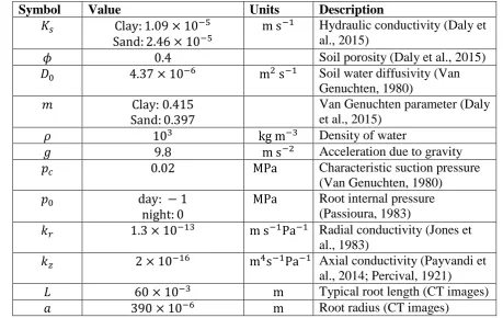
vector in the direction of gravity. The mathematical symbols, their meaning and units are 261
summarised in Table 1. 262
263
The root exerts a suction pressure given by equation (3) on the soil. This induces a pressure 264
drop across the soil and acts to draw water into the root. This pressure is related to the 265
suction through the Van-Genuchten equation (Van Genuchten, 1980) which, on the surface 266
of the root, can be written as 267
−𝒏̂ ⋅ [𝐷0𝐷(𝑆)𝛁𝑆 − 𝐾𝑠𝐾(𝑆)𝒆̂𝑧] = 𝑘𝑟(𝑝𝑐𝑓(𝑆) − 𝑝0), (8)
268
13 𝑓(𝑆) = (𝑆−𝑚1 − 1 )
1−𝑚
. (9)
270
The remaining external boundaries are assumed to be impermeable to fluid, hence we write 271
𝒏̂ ⋅ 𝒖 = 0 on the outer pot boundary. The boundary condition at the bottom is 𝒏̂ ⋅ 𝒖 = 𝐾(𝑆), 272
i.e., the only water flux at the bottom of the pot is due to gravity and at the top 𝒏̂ ⋅ 𝒖 = 𝑞𝑠 273
where 𝑞𝑠(𝑡) is the flux of water into the soil. We use, as an initial condition, 𝑆 = 0.5 274
corresponding to a plant which has been recently watered and consider the case 𝑞𝑠(𝑡) = 0.
275
276
The parameters used in these equations are taken from the literature and previous studies on 277
soil water imaging. Specifically we use 𝑘𝑟 = 1.3 × 10⁻¹³m s−1Pa−1 (Jones et al., 1983),
278
𝑘𝑧 = 2 × 10⁻¹⁶m4 s−1 Pa−1 (Payvandi et al., 2014; Percival, 1921). The soil water
279
diffusivity, 𝐷0, is taken directly from the literature and is set to 𝐷0 = 4.37 × 10⁻⁶ m2s−1 280
(Van Genuchten, 1980). The hydraulic conductivity, 𝐾𝑠, and the Van-Genuchten parameter,
281
𝑚, are taken from Daly et al. (2015) for the two different soil types. Specifically we use 282
𝑚 =0.415 and 𝐾𝑠 = 1.09 × 10⁻⁵ m s−1 for the clay loam and 𝑚 = 0.397 and 𝐾𝑠 =
283
2.46 × 10⁻⁵ m s−1 for the loamy sand soil.
284
285
The equations described above are implemented directly on the numerical meshes generated 286
by Simpleware. Water uptake is simulated for a period of one day to calculate uptake over a 287
single day-night cycle which consists of a 16 hour day and 8 hour night corresponding to the 288
growth conditions. At night water uptake is assumed to be zero and evaporation is assumed 289
to be zero throughout the simulation. The equations were solved using Comsol Multiphysics 290
14 run on a single 16 processor node of the Iridis 4 supercomputing cluster at the University of 292
Southampton to calculate the water profile in the soil and root water uptake. Resource usage 293
varied dependent on the complexity of the root geometry, the most expensive simulations 294
used ≈ 90 Gb of memory and ran in under 60 hours. 295
296
3.4.3. Comparison with spatially averaged model 297
In order to quantify the effects of including the root architecture explicitly we compare our 298
results to the averaged model developed in Roose and Fowler (2004). This averaged model is 299
based on the observation that, for sufficiently small inter-root spacing, any saturation 300
gradients in the horizontal direction will equilibrate sufficiently quickly that variations in this 301
direction may be neglected. The averaged model is derived by assuming that the uptake 302
properties of the root system are equal across the whole root surface. This does not mean that 303
the uptake across the root is equal. Rather, it is dependent on the soil water pressure which 304
may vary with depth. Hence, the one dimensional equation for root water uptake is given by 305
𝜙𝜕𝑆
𝜕𝑡+ 𝛁 ⋅ [𝐷0𝐷(𝑆)𝛁𝑆 − 𝐾𝑠𝐾(𝑆)𝒆̂𝑧] = 𝐴𝑒𝑓𝑓𝑘𝑟(𝑝𝑐𝑓(𝑆) − 𝑝0),
(10) 306
where 𝐴𝑒𝑓𝑓 = 𝐿𝑟𝐴𝑝𝐴𝑟 , 𝐴𝑟 is the root surface area, 𝐴𝑝 is the cross sectional area of the pot and 𝐿𝑟
307
is the root length. For direct comparison with the image based method these equations are 308
solved in Comsol Multiphysics using the same implementation method as described above. 309
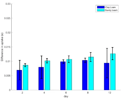
In order to compare the two methods we define the difference in cumulative uptake as 310
𝑒 =2(𝐼𝐴− 𝐼𝐼) (𝐼𝐼+ 𝐼𝐴)
15 where 𝐼𝐴 and 𝐼𝐼 are the total uptake for the averaged model and the image based model 311
respectively. 312
313
3.4.4. Statistical Analysis 314
The results obtained experimentally were analysed by general analysis of variance 315
(ANOVA) containing soil type, time period and all possible interactions as explanatory 316
variables using Genstat 15.1 (VSN International, UK). The probability of significance P, 317
with a threshold value of (P<0.05), corresponding to a 95% confidence limit, was calculated 318
and is used as a measure of significance of results obtained. 319
320
4. Results & Discussion 321
322
4.1.Soil pore geometry 323
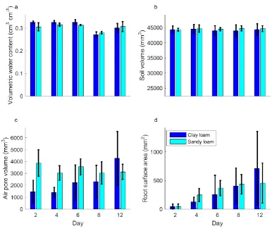
No significant changes in soil volume from the imaging method were recorded across the 324
experiment, confirming structural changes were due to alterations in the pore size distribution 325
(Figure 1). Throughout the 12 days the average volume of air, imaged in the form of 326
macropores, remained approximately constant in the loamy sand soil (Figure 1). Whilst there 327
was large variation within treatment from day 2 until day 8, the average volume of imaged air 328
filled pores was greater in the loamy sand soil than the clay soil (P<0.01). However, at day 12 329
this trend switched, so that the average air filled pore volume in a clay sample was 4268 mm3 330
compared to just 3130 mm3 in the loamy sand soil. From a visual inspection of the X-ray CT 331
images this increase in air filled pore volume at day 12, after the samples have undergone 332
16 swelling and shrinking properties (see supplementary figures 1 and 2 for greyscale images) 334
and is potentially linked to soil drying through root water uptake. 335
336
4.2.Root system architecture 337
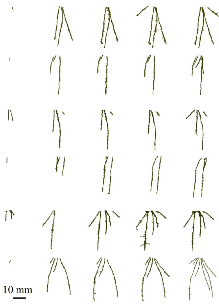
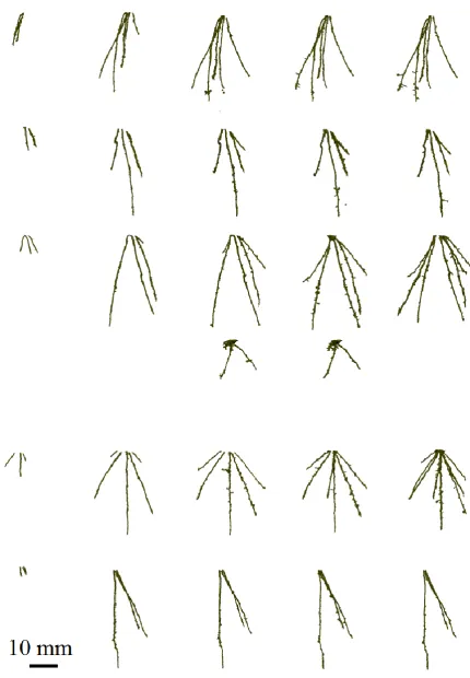
The scanned root architectures for plants grown in the loamy sand and clay loam are shown 338
in Figure 2 and Figure 3 respectively. No significant differences in root measurements were 339
found between samples that had undergone X-ray CT scanning and those that had not 340
(P>0.05), suggesting no harmful effects of X-ray dose on the plants (see supplementary table 341
S1 for details). Root volumes as quantified by WinRHIZO™ were greater for plants grown 342
in clay soil than for those grown in loamy sand soil (P<0.05). However, no significant 343
differences were observed in root volume measured using X-ray CT. It would not be useful 344
to draw comparisons between root measurements obtained via destructive root sampling 345
(WinRHIZO™) and the non-destructive X-ray CT scanning due to the inherent differences in 346
the techniques (e.g. 2D vs. 3D, in soil and without soil etc.), (Tracy et al., 2012). Using X-ray 347
CT we observed a significant difference (710 mm2 vs. 455 mm2; P<0.05) in root surface area 348
for plants grown in a clay loam compared to the loamy sand soil (Figure 1). Based on the CT 349
images the majority of growth took place in the first four days. Ideally, a higher frequency of 350
scans at this point in the root development would have facilitated a clearer picture of root 351
growth. However, due to the cost and time taken to scan and process this data we were not 352
able to obtain additional scans in the first four days. 353
354
We did not observe fine lateral roots in the CT scans due to the resolution. However, it is 355
17 (Payvandi et al., 2014; Sevanto, 2014; Thompson and Holbrook, 2003). As a result, water 357
movement in fine laterals will be much slower than the primary roots. Hence, it has been 358
suggested that fine laterals are less important in terms of water uptake (Roose and Fowler, 359
2004). The increase in measured root mass comes directly from an increase in the primary 360
roots. Over the course of the experiments the roots did not become pot bound; this was 361
evidenced through measuring maximum width and depth of the root system. The average 362
width at day 12 was 39 mm, which was less than the pot diameter of 50 mm, and the average 363
depth at day 12 was 47 mm, which was less than the pot depth of 80 mm. 364
365
4.3.Root water uptake 366
Over the 12 day experiment the watering regime remained constant. However, at day 8 a 367
reduction in water content was measured via imaging (Figure 1; P<0.001). It is possible that, 368
at day 8, the plant stopped being reliant on seed reserves and began capturing resources from 369
the soil (Kennedy et al., 2004). However, we observed that this reduction in water content 370
disappeared at day 12. It is possible that a temporary increase in the rate of water uptake 371
occurs at this time, possibly related to the formation of lateral roots. However there is not 372
sufficient evidence to confirm this and the dip may simply be a result of 373
imaging/segmentation errors or minor differences in the watering regime. Hence, further 374
investigation is needed to quantify these effects. 375
376
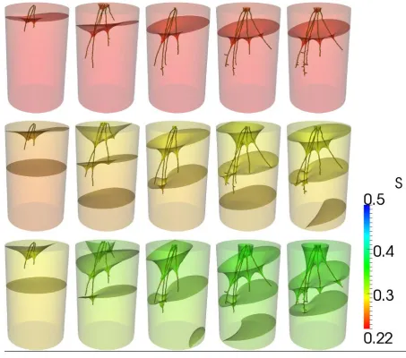
To quantify the regions from which water has been taken we consider the numerical 377
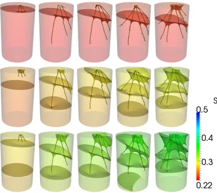
simulations. We visualised the water distribution within the soil by calculating regions of 378
18 show up as surfaces. We visualised these surfaces at different times after watering in Figure 380
4, Figure 5 and the supplementary material. These surfaces are plotted for a single plant at 2, 381
4, 6, 8 and 12 days after planting for three different times within the uptake cycle. A clear 382
depletion in water content was observed over the course of a day. 383
384
In addition, the simulations show that water content is lower near the roots generating a net 385
flux of water towards the plant. This lower moisture content in the region immediately 386
adjacent to the root is in line with the observation that water content in the rhizosphere is 387
lower than the moisture content far from the root (Carminati, 2012; Moradi et al., 2011). 388
However, we note that in these simulations we do not explicitly treat the soil adjacent to the 389
root differently to the soil far from the root. This effect is more pronounced in the clay soil 390
(Figure 5), than the loamy sand (Figure 4) and can be seen by the density of the equal 391
saturation surfaces in the figures. 392
393
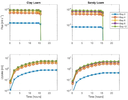
In order to quantify the uptake rate and total uptake of the roots over the course of the day-394
night, we calculated the flux and cumulative uptake, averaged over all replicates, for the clay 395
loam and loamy sand soils (Figure 6 and supplementary material). The largest change in 396
water uptake, based on simulation, occurs in the first four days of root development. We note 397
that, due to the watering regime, these changes will not be echoed in the volumetric water 398
content, Figure 1. Whilst there are still changes after this point, these are not as pronounced. 399
We do not observe any dip in water uptake at day 8. This suggests that the observed decrease 400
in volumetric water content is due to processes which are not being measured. Whilst it is 401
tempting to attribute this difference to the presence of fine laterals, this does not explain the 402
19 the X-ray CT imaging, will be significantly smaller than the primary roots observed. 404
Therefore, their conductivity, and contribution to uptake, would be significantly smaller than 405
that of the primary roots. 406
407
In order to quantify how the details of the root geometry affected water uptake, we compared 408
the uptake predicted using these models to water uptake predicted by the simplified water 409
uptake model developed by Roose and Fowler (2004). We consider water uptake over a 24 410
hour period. At the start of the simulation the water content is assumed constant over the root 411
system with saturation S=0.5 throughout. This is comparable to the growth conditions in the 412
columns which were rewatered to a known weight on a daily basis. The water content would 413
then decrease due to a combination of water uptake and loss via drainage or evaporation over 414
the 24 hour period. To facilitate the most direct comparison of the two methods we have 415
used the root surface area extracted from the X-ray CT data to parameterise the model. This 416
means that we are directly comparing how the geometrical properties of the root systems 417
affect uptake and flux. The averaged and image based models agree well in terms of total 418
uptake, Figure 6 and Figure 7. The difference in cumulative uptake defined in equation (11) 419
is less than 2%, Figure 7. 420
421
In general, the imaged geometry predicts a smaller uptake than the averaged geometry. The 422
largest difference is observed for the older plants, ≈ 1.25% for the plants grown in the sandy 423
loam and ≈ 1% for the plants grown in clay loam. The difference is even smaller for the 424
younger plants <1% for both soil types. To put this difference in context, the error for 425
Neutron Magnetic Resonance imaging (NMRi) of water uptake is approximately 7% 426
20 Neutron probes and Time Domain Reflectometry can be as high as 12% (Smethurst et al,. 428
2006). There is also a wealth of information that cannot be investigated using the averaged 429
models. In particular the local distribution of water around the root cannot be investigated by 430
the averaged models. This means that any effect of soil inhomogeneity in the rhizosphere or 431
crack formation, due to soil shrinkage and swelling, will be neglected. Hence, the use of 432
averaged models is reasonable if the quantity of interest is simply the absolute uptake by the 433
root system. 434
435
Image based modelling allows water uptake by plants to be calculated using observed root 436
geometries and, in this study, provides comparable results to the averaged models. However, 437
there are sources of error present in image based modelling which need to be considered 438
carefully when interpreting these results. Firstly, the outputs of the uptake model are, at best, 439
only as accurate as the imaging and segmentation procedures. As it is only possible to model 440
what is observed, the segmented root system does not represent the full root system as fine 441
lateral roots and root hairs will not be captured at the resolution of these scans. Hence, the 442
contribution of these features of the root geometry to plant water uptake will not be captured. 443
However, as the transport of water by plant roots scales with the fourth power of the root 444
radius, we would expect that any sub resolution fine laterals would be insignificant. To 445
quantify this we consider the uptake of roots at the limit of resolution. The roots which we 446
do consider fall into the category of large thick roots, equation (1). Hence, their uptake is 447
limited by the availability of water to the root. For the case of fine laterals of radius 30 µm 448
we find 𝜅2 = 12.6, where we have scaled 𝑘𝑧 to take into account the reduced root radius. 449
This corresponds to small thin roots which have been shown, (Roose and Fowler, 2004), to 450
only take up water in a region of length 𝐿𝑢 ∝ 1/𝜅 near to the base of the roots. Hence, the
451
21 uptake where they join the primary roots. Whilst it is not possible to precisely quantify this 453
uptake, it is expected to be small compared to the relative errors of imaging, segmentation 454
and meshing. Secondly, whilst every care has been taken to segment the roots in a 455
reproducible and robust way, and every effort taken to minimise minor differences in signal-456
to-noise ratio between scans, no segmentation procedure is perfect. Finally, the assumptions 457
used in this model such as soil homogeneity, uniform initial conditions and stationary root 458
architecture are not necessarily realistic and will introduce errors into the results. Some of 459
these limitations could be overcome using higher resolution X-ray CT imaging, but the trade-460
off between sample diameter and achievable resolution would remain, or by adapting the 461
models to consider growing root architectures through interpolation (Daly et al., 2016) or 462
repeated imaging (Koebernick et al., 2015). 463
464
Conclusions 465
In this paper we have shown that, for pots of 50 mm diameter, differences in plant water 466
uptake can be observed between a spatially averaged model and an image based model. 467
These differences can be quantified both in terms of uptake rate and cumulative uptake. The 468
difference between the averaged and image based models was less than 2% for all cases 469
considered, this is less than typical experimental error in plant water uptake measurements. 470
The averaging methods were not able to resolve the soil moisture profile in three dimensions 471
meaning that they would be unable to truly capture heterogeneity in the rhizosphere. Hence, 472
whilst averaging is a useful method for quickly estimating water uptake, there is significant 473
information lost which may be important in terms of understanding rhizosphere function. 474
22 There are several assumptions in the image based models and there is room for improvement. 476
In principle the numerical modelling in this paper could be extended to older plants with 477
much larger root systems and could include root growth through an effective growth rate into 478
the model, a method which has been used to study nutrient uptake by root hairs (Daly et al., 479
2016). However, despite the assumptions present, non-destructive imaging combined with 480
image based modelling remains a powerful tool to not only visualise soil geometry but to 481
quantify the effects of the observable root architecture on plant water uptake. 482
483
5. Acknowledgements 484
The authors acknowledge the use of the IRIDIS High Performance Computing Facility, and 485
associated support services at the University of Southampton, in the completion of this work. 486
This project was funded by BBSRC BB/J000868/1, a collaborative project between the 487
Universities of Southampton and Nottingham, PI and overall lead TR. KRD and TR are also 488
funded by ERC consolidation grant 646809DIMR. 489
490
Data Accessibility 491
All reconstructed scan data will be available on request by emailing 492
[email protected]. For simulation results please email [email protected]. 493
494
6. References 495
Arbogast, T. and Lehr, H. L. (2006). Homogenization of a Darcy–Stokes system 496
modeling vuggy porous media. Computational Geosciences 10, 291-302. 497
Carminati, A. (2012). A model of root water uptake coupled with rhizosphere 498
23 Cioranescu, D. and Donato, P. (1999). An introduction to homogenization: Oxford 500
University Press Oxford. 501
Czarnes, S., Hallett, P. D., Bengough, A. G. and Young, I. M. (2000). Root- and 502
microbial-derived mucilages affect soil structure and water transport. European Journal of
503
Soil Science 51, 435-443. 504
Daly, K. R., Keyes, S. D., Masum, S. and Roose, T. (2016). Image-based modelling 505
of nutrient movement in and around the rhizosphere. Journal of experimental botany 67, 506
1059-1070. 507
Daly, K. R., Mooney, S., Bennett, M., Crout, N., Roose, T. and Tracy, S. (2015). 508
Assessing the influence of the rhizosphere on soil hydraulic properties using X-ray Computed 509
Tomography and numerical modelling. Journal of experimental botany 66, 2305-2314. 510
Daly, K. R. and Roose, T. (2014). Multiscale modelling of hydraulic conductivity in 511
vuggy porous media. Proceedings of the Royal Society A: Mathematical, Physical and
512
Engineering Science 470(2162), 20130383. 513
Daly, K. R. and Roose, T. (2015). Homogenization of two fluid flow in porous 514
media 471(2176) 20140564. 515
Dexter, A. (1987). Compression of soil around roots. Plant and Soil 97, 401-406. 516
Doussan, C., Pierret, A., Garrigues, E. and Pagès, L. (2006). Water uptake by plant 517
roots: II–modelling of water transfer in the soil root-system with explicit account of flow 518
within the root system–comparison with experiments. Plant and Soil 283, 99-117. 519
Downie, H. F., Adu, M. O., Schmidt, S., Otten, W., Dupuy, L. X., White, P. J. and 520
Valentine, T. A. (2014). Challenges and opportunities for quantifying roots and rhizosphere 521
interactions through imaging and image analysis. Plant Cell Environ 38(7) 1213-1232. 522
Gregory, P. (2006). Roots, rhizosphere and soil: the route to a better understanding of 523
soil science? European Journal of Soil Science 57, 2-12. 524
Hiltner, L. (1904). Über neuere Erfahrungen und Probleme auf dem Gebiete der 525
Bodenbakteriologie unter besonderer Berücksichtigung der Gründüngung und Brache. 526
Arbeiten der Deutschen Landwirtschaftlichen Gesellschaft 98, 59-78. 527
Hornung, U. (1997). Homogenization and porous media: Springer. 528
Jones, H., Tomos, A. D., Leigh, R. A. and Jones, R. G. W. (1983). Water-relation 529
parameters of epidermal and cortical cells in the primary root ofTriticum aestivum L. Planta
530
158, 230-236. 531
Keller, J. B. (1980). Darcy’s law for flow in porous media and the two-space method. 532
In Nonlinear partial differential equations in engineering and applied science (Proc. Conf.,
533
Univ. Rhode Island, Kingston, RI, 1979), vol. 54, pp. 429-443: Dekker New York. 534
Kennedy, P., Hausmann, N., Wenk, E. and Dawson, T. (2004). The importance of 535
seed reserves for seedling performance: an integrated approach using morphological, 536
physiological, and stable isotope techniques. Oecologia 141, 547-554. 537
Koebernick, N., Huber, K., Kerkhofs, E., Vanderborght, J., Javaux, M., 538
Vereecken, H. and Vetterlein, D. (2015). Unraveling the hydrodynamics of split root water 539
uptake experiments using CT scanned root architectures and three dimensional flow 540
simulations. Frontiers in plant science 6, 370. 541
Landsberg, J. and Fowkes, N. (1978). Water movement through plant roots. Annals
542
of Botany 42, 493-508. 543
Lewis, J. and Sjostrom, J. (2010). Optimizing the experimental design of soil 544
columns in saturated and unsaturated transport experiments. Journal of Contaminant
545
Hydrology 115, 1-13. 546
Mairhofer, S., Zappala, S., Tracy, S. R., Sturrock, C., Bennett, M., Mooney, S. J. 547
24 Architecture in Soil from X-Ray Microcomputed Tomography Images Using Visual 549
Tracking. Plant Physiology 158, 561-569. 550
Mooney, S. J. and Morris, C. (2008). A morphological approach to understanding 551
preferential flow using image analysis with dye tracers and X-ray Computed Tomography. 552
CATENA 73, 204-211. 553
Mooney, S. J., Pridmore, T. P., Helliwell, J. and Bennett, M. J. (2012). 554
Developing X-ray Computed Tomography to non-invasively image 3-D root systems 555
architecture in soil. Plant and Soil 352, 1-22. 556
Moradi, A. B., Carminati, A., Vetterlein, D., Vontobel, P., Lehmann, E., Weller, 557
U., Hopmans, J. W., Vogel, H. J. and Oswald, S. E. (2011). Three‐dimensional 558
visualization and quantification of water content in the rhizosphere. New Phytologist 192, 559
653-663. 560
Mualem, Y. (1976). A new model for predicting the hydraulic conductivity of 561
unsaturated porous media. Water Resources Research 12, 513-522. 562
Panfilov, M. (2000). Macroscale models of flow through highly heterogeneous 563
porous media: Springer. 564
Passioura, J. (1983). Roots and drought resistance. Agricultural water management
565
7, 265-280. 566
Pavliotis, G. and Stuart, A. (2008). Multiscale methods: averaging and 567
homogenization: Springer Science & Business Media. 568
Payvandi, S., Daly, K. R., Jones, D., Talboys, P., Zygalakis, K. and Roose, T. 569
(2014). A mathematical model of water and nutrient transport in xylem vessels of a wheat 570
plant. Bulletin of mathematical biology 76, 566-596. 571
Percival, J. (1921). The wheat plant: a monograph No. SB4191. W5 P4). 572
Richards, L. A. (1931). Capillary conduction of liquids through porous mediums. 573
Journal of Applied Physics 1, 318-333. 574
Rogasik, H., Crawford, J. W., Wendroth, O., Young, I. M., Joschko, M. and Ritz, 575
K. (1999). Discrimination of soil phases by dual energy x-ray tomography. Soil Science
576
Society of America Journal 63, 741-751. 577
Roose, T. and Fowler, A. (2004). A model for water uptake by plant roots. Journal
578
of theoretical biology 228, 155-171. 579
Roose, T. and Schnepf, A. (2008). Mathematical models of plant–soil interaction. 580
Philosophical Transactions of the Royal Society A: Mathematical, Physical and Engineering
581
Sciences 366, 4597-4611. 582
Rowse, H., Stone, D. and Gerwitz, A. (1978). Simulation of the water distribution in 583
soil. Plant and Soil 49, 533-550. 584
Sevanto, S. (2014). Phloem transport and drought. Journal of experimental botany, 585
65(7) 1751-1759. 586
Scheenen, T. W. J., D. Van Dusschoten, P. A. De Jager, and H. Van As. "Quantification of 587
water transport in plants with NMR imaging." Journal of Experimental Botany 51, no. 351 (2000): 588
1751-1759. 589
Smethurst, J.A., Clarke, D. and Powrie, W. (2006). Seasonal changes in pore water 590
pressure in a grass covered cut slope in London Clay. Géotechnique, 56(8), 523-537. 591
Stirzaker, R. J., Passioura, J. B. and Wilms, Y. (1996). Soil structure and plant 592
growth: Impact of bulk density and biopores. Plant and Soil 185, 151-162. 593
Thompson, M. and Holbrook, N. (2003). Scaling phloem transport: water potential 594
equilibrium and osmoregulatory flow. Plant Cell Environ 26, 1561-1577. 595
Tracy, S. R., Daly, K. R., Sturrock, C. J., Crout, N. M. J., Mooney, S. J. and 596
Roose, T. (2015). Three dimensional quantification of soil hydraulic properties using X-ray 597
Computed Tomography and image based modelling Water Resources Research 51(2)
1006-598
25 Tracy S.R., Black C.R., Roberts J.A., Sturrock C., Mairhofer S., Craigon J., 600
Mooney S.J. (2012). Quantifying the impact of soil compaction on root system architecture 601
in tomato (Solanum lycopersicum L.)by X-ray micro- Computed Tomography (CT). Annals
602
of Botany. 110, 511-519. 603
Van Genuchten, M. T. (1980). A closed-form equation for predicting the hydraulic 604
conductivity of unsaturated soils. Soil science society of America journal 44, 892-898. 605
Veihmeyer, F. and Hendrickson, A. (1931). The moisture equivalent as a measure 606
of the field capacity of soils. Soil Science 32, 181-194. 607
Vereecken, H., Schnepf, A., Hopmans, J.W., Javaux, M., Or, D., Roose, T., …, 608
Young, I.M. (2016) Modeling soil processes: key challenges and new perspectives. Vadose
609
Zone Journal 15(5). 610
Walker, T. S., Bais, H. P., Grotewold, E. and Vivanco, J. M. (2003). Root 611
exudation and rhizosphere biology. Plant Physiology 132, 44-51. 612
Whalley, W., Ober, E. and Jenkins, M. (2013). Measurement of the matric potential 613
of soil water in the rhizosphere. Journal of experimental botany 64, 3951-3963. 614
Whalley, W. R., Riseley, B., Leeds‐Harrison, P. B., Bird, N. R., Leech, P. K. and 615
Adderley, W. P. (2005). Structural differences between bulk and rhizosphere soil. European
616
Journal of Soil Science 56, 353-360. 617
Young, I. M. (1995). Variation in moisture contents between bulk soil and the 618
rhizosheath of wheat (Triticum-aestivum L cv Wembley). . New Phytologist 130, 135-139. 619
Zappala, S., Helliwell, J. R., Tracy, S. R., Mairhofer, S., Sturrock, C. J., 620
Pridmore, T., Bennett, M. and Mooney, S. J. (2013). Effects of X-ray dose on rhizosphere 621
studies using X-ray computed tomography. PloS one 8, E67250. 622
26 Figures
626 627
628
Figure 1 Imaged data for (a) volumetric water content, (b) soil volume, (c) air volume, and (d) root surface area.
[image:26.595.96.483.128.456.2]27 631
[image:27.595.75.519.69.691.2]632 633
Figure 2: Root architectures for roots grown in loamy sand soil. Each row is a different sample. Columns correspond to
634
Day 2, Day 4, Day 6, Day 8, Day 12. Scale bar is 10 mm.
28 636
637
[image:28.595.84.515.68.689.2]
638
Figure 3: Root architectures for roots grown in clay loam soil. Each row is a different sample. Columns correspond to
639
Day 2, Day 4, Day 6, Day 8, Day 12. Scale bar is 10 mm.
29 641
642
[image:29.595.67.521.96.496.2]643
Figure 4: Water saturation (S) in loamy sand soil for a growing root system. Left to right shows the root system at 2, 4, 6,
644
8 and 12 days post transplanting. Images from top to bottom show half an hour of simulation, 6 hours of simulation and
645
12 hours of simulation. The images show the total geometry modelled, i.e., the pot (50 mm diameter, 80 mm height)
646
with the root architecture inside. The surfaces show regions of equal saturation with the colour representing the
647
saturation at that point within the pot.
30 651
Figure 5: Water saturation (S) in a clay loam soil for a growing root system. Left to right shows the root system at 2, 4, 6,
652
8 and 12 days post transplanting. Images from top to bottom show half an hour of simulation, 6 hours of simulation and
653
12 hours of simulation. The images show the total geometry modelled, i.e., the pot (50 mm diameter, 80 mm height)
654
with the root architecture inside. The surfaces show regions of equal saturation with the colour representing the
655
saturation at that point within the pot.
31 659
Figure 6 Water flux (top) and cumulative uptake (bottom) over a single day-night cycle for Clay loam (left) and loamy
660
sand (right) soils. The data has been calculated using the image based modelling approach taking into account the full
661
root geometry. Data is shown for 2, 4, 6, 8 and 12 days post transplantation. .
32 663
[image:32.595.94.485.86.409.2]664
Figure 7 Relative difference in cumulative uptake (e), as defined by equation (11). The data shows the difference
665
between the image based and averaged models for clay loam and loamy sand soils.
33
Table 1: Parameter values
668
Symbol Value Units Description
𝐾𝑠 Clay: 1.09 × 10⁻⁵
Sand: 2.46 × 10⁻⁵ m s
−1 Hydraulic conductivity (Daly et
al., 2015)
𝜙 0.4 Soil porosity (Daly et al., 2015)
𝐷0 4.37 × 10⁻⁶ m2 s−1 Soil water diffusivity (Van
Genuchten, 1980)
𝑚 Clay: 0.415
Sand: 0.397
Van Genuchten parameter (Daly et al., 2015)
𝜌 103 kg m−3 Density of water
𝑔 9.8 m s−2 Acceleration due to gravity
𝑝𝑐 0.02 MPa Characteristic suction pressure
(Van Genuchten, 1980)
𝑝0 day: − 1
night: 0 MPa
Root internal pressure (Passioura, 1983)
𝑘𝑟 1.3 × 10⁻¹³ m s−1Pa−1 Radial conductivity (Jones et
al., 1983)
𝑘𝑧 2 × 10⁻¹⁶ m4s−1Pa−1 Axial conductivity (Payvandi et
al., 2014; Percival, 1921)
𝐿 60 × 10−3 m Typical root length (CT images)
𝑎 390 × 10−6 m Root radius (CT images)