Fast algorithms for fitting active appearance models to unconstrained images

DOI 10.1007/s11263-016-0950-1

Fast Algorithms for Fitting Active Appearance Models

to Unconstrained Images

Georgios Tzimiropoulos1 · Maja Pantic2,3

Received: 24 March 2014 / Accepted: 3 September 2016

© The Author(s) 2016. This article is published with open access at Springerlink.com

Abstract Fitting algorithms for Active Appearance Mod-els (AAMs) are usually considered to be robust but slow or fast but less able to generalize well to unseen variations. In this paper, we look into AAM fitting algorithms and make the following orthogonal contributions: We present a simple “project-out” optimization framework that unifies and revises the most well-known optimization problems and solutions in AAMs. Based on this framework, we describe robust simul-taneous AAM fitting algorithms the complexity of which is not prohibitive for current systems. We then go on one step further and propose a new approximate project-out AAM fit-ting algorithm which we coin Extended Project-Out Inverse Compositional (E-POIC). In contrast to current algorithms, E-POIC is both efficient and robust. Next, we describe a part-based AAM employing a translational motion model, which results in superior fitting and convergence proper-ties. We also show that the proposed AAMs, when trained “in-the-wild” using SIFT descriptors, perform surprisingly well even for the case of unseen unconstrained images. Via a number of experiments on unconstrained human and ani-mal face databases, we show that our combined contributions largely bridge the gap between exact and current approximate methods for AAM fitting and perform comparably with state-of-the-art face alignment systems.

Communicated by Yuri Boykov.

B

[email protected]

1 _{School of Computer Science, University of Nottingham,} Nottingham, UK

2 _{Department of Computing, Imperial College London,} London, UK

3 _{Faculty of Electrical Engineering, Mathematics and Computer} Science, University of Twente, Enschede, The Netherlands

Keywords Active Appearance Models·Face alignment· In-the-wild

1 Introduction

Pioneered byCootes et al.(2001) and revisited byMatthews and Baker(2004), Active Appearance Models (AAMs) have been around in computer vision research for more than 15 years. They are statistical models of shape and appearance that can generate instances of a specific object class (e.g. faces) given a small number of model parameters. Fitting an AAM to a new image entails estimating the model para-meters so that the model instance and the given image are “close enough” typically in a least-squares sense. Recov-ering the shape parameters is important because it implies that the location of a set of landmarks (or fiducial points) has been detected in the given image. Landmark localiza-tion is of fundamental significance in many computer vision problems like face and medical image analysis. Hence, fit-ting AAMs robustly to new images has been the focus of extensive research over the past years.

Of particular interest in this work is the second line of research for fitting AAMs through non-linear least-squares (Matthews and Baker 2004). In particular, AAM fitting is for-mulated as a Lucas–Kanade (LK) problem (Lucas et al. 1981) which can be solved iteratively using Gauss–Newton opti-mization. However, standard gradient descend algorithms when applied to AAM fitting are inefficient. This problem was addressed in the seminal work ofMatthews and Baker (2004) which extends the LK algorithm and the

appearance-based tracking framework ofHager and Belhumeur(1998)

for the case of AAMs and deformable models. One of the major contributions ofMatthews and Baker(2004) is the so-called Project-Out Inverse Compositional algorithm (POIC). The algorithm is coined project-out because it decouples shape from appearance and inverse compositional because the update is estimated in the model coordinate frame and then composed to the current estimate (this is in contrast to the standard LK algorithm in which the parameters are updated in a forward additive fashion). The combination results in an algorithm which is as efficient as regression-based approaches and is now considered the standard choice for fitting person-specific AAMs (i.e. AAMs for modeling a specific subject known in advance during training). Its main disadvantage is its limited capability of generalizing well to unseen variations, the most notable example of which is the case of generic AAMs (i.e. AAMs for modeling subjects not seen during training).

In contrast to POIC, the Simultaneous Inverse Composi-tional (SIC) algorithm (Baker et al. 2003) has been shown to perform robustly for the case of generic fitting (Gross et al. 2005). However, the computational cost of the algorithm is almost prohibitive for most applications. Letnandmdenote the number of the shape and appearance parameters of the AAM. Then, the cost per iteration for SIC isO((n+m)2N), whereNis the number of pixels in the reference frame. Note that the cost of POIC is only O(n N). For generic fitting mnand hence the huge difference in computational cost has either ruled out SIC from most papers/studies that depart from the person-specific case or made the authors resort in approximate solutions (please see (Saragih and Gocke 2009) for an example).

Some attempts to reduce the cost of SIC do exist but they are limited. An example is the Normalization algorithm (Gross et al. 2005). However, the performance of the Nor-malization algorithm has been reported to be closer to that of POIC rather than that of SIC. A second notable example isPapandreou and Maragos(2008) which applies the update rules originally proposed inHager and Belhumeur(1998) to the problem of AAM fitting. The framework proposed in this paper is also based onHager and Belhumeur(1998), but it extends it in several different ways (please see below for a summary of our contributions). Finally, other techniques for reducing the cost to some extent via pre-computations have

been reported inBatur and Hayes (2005) andNetzell and Solem(2008).

1.1 Summary of Contributions and Paper Roadmap

In this paper, we attempt to address two important questions in AAM literature:

1. Can AAMs provide fitting performance comparable to that of contemporary state-of-the-art algorithms for the difficult problem of fitting facial deformable models to unconstrained images (also known as face alignment in-the-wild)?

2. What is the relation between performance and computa-tional efficiency? How efficient can exact algorithms be? More importantly, are there any inexact algorithms that are also robust?

In the remaining of this paper, we show that the answer to the above questions is positive, however multiple con-tributions/improvements in almost orthogonal directions are necessary in order to achieve both aims. In particular, our contributions include:

1. Two approximate but both robust and efficient fitting algorithms coined approximate Fast-SIC (aFast-SIC) and

Extended POIC (E-POIC) with complexity O((n +

m)N +n2N)and O(n N), respectively. We show that aFast-SIC has essentially the same fitting and conver-gence properties as SIC, and can be seen as a block coordinate descent algorithm for AAM fitting. Addi-tionally, we show that E-POIC largely bridges the gap between SIC and POIC, and can be seen as a very fast regression-based approach to AAM fitting.

2. Robust training of AAMs. In particular, we propose a new direction for employing AAMs in unconstrained conditions by means of training AAMs in-the-wild, and provide justifications why such a training procedure is beneficial for AAM fitting.

3. Part-based AAMs combined with a translational motion model (as opposed to standard holistic AAMs with piece-wise affine warp). We show that our part-based AAM, coined Gauss–Newton Deformable Part Model (GN-DPM), is more robust and accurate and has superior convergence properties.

Having summarized the individual contributions of our paper above, we are now ready to state the main result of our paper: Our part-based AAM (GN-DPM) built from SIFT features and fitted with the E-POIC algorithm has essentially the same fitting performance as the same model fitted with aFast-SIC. Although E-POIC requires a few more iterations to converge, it is very efficient (O(n N)) and almost two orders of magni-tude faster per iteration than aFast-SIC. Finally, in terms of fitting accuracy, both algorithms are shown to achieve state-of-the-art performance, and sometimes superior to that of two state-of-the-art methods, namely SDM (Xiong and De la Torre 2013) and Chehra (Asthana et al. 2014). In addi-tion to human faces, our results are also verified on a newly collected and very challenging animal face data set.

Following Sects.2–4which provide related work in face alignment and AAMs, the aforementioned contributions are described in the following sections:

1. In Sect.5, we present a simple optimization framework for AAM fitting that unifies and revises the most well-known optimization problems and solutions in AAMs. Our framework derives and solves the optimization prob-lem for Fast-SIC, a fast algorithm that is theoretically guaranteed to provide exactly the same updates per itera-tions as the ones provided by SIC, and describes a simple and approximate Fast-SIC algorithm coined aFast-SIC. 2. In Sect. 6, and based on the analysis of Sect. 5, we

describe our approximate but both robust and efficient AAM fitting algorithm coined E-POIC.

3. In Sect.7, we illustrate the benefits of the proposed train-ing of AAMs in-the-wild.

4. In Sect.8.1, we describe the proposed part-based AAM, coined GN-DPM, and show how this model can be fit-ted with Gauss–Newton optimization via a translational motion model.

5. In Sect.9, we describe the efficient fitting of SIFT-based AAMs based on a weighted least-squares formulation. 6. In Sect.10, we report experiments illustrating the fitting

and convergence properties of all AAMs described in this work and provide comparisons with state-of-the-art.

Finally, we conclude in Sect.11. Portions of this work appear in two conference publications, please seeTzimiropoulos and Pantic(2013) andTzimiropoulos and Pantic(2014).

2 State-of-the-Art in Face Alignment

The problem of face alignment has a long history in com-puter vision and a large number of approaches have been proposed to tackle it. Typically, faces are modelled as deformable objects which can vary in terms of shape and appearance. Much of early work revolved around the Active

Shape Models (ASMs) and the AAMs (Cootes et al. 1995, 2001; Matthews and Baker 2004). In ASMs, facial shape is expressed as a linear combination of shape bases learned via principal component analysis (PCA), while appearance is modelled locally using (most commonly) discriminatively learned templates. In AAMs, shape is modelled as in ASMs but appearance is modelled globally using PCA in a canonical coordinate frame where shape variation has been removed. More recently, the focus has been shifted to the family of methods coined Constrained Local Models (CLMs) (Cristi-nacce and Cootes 2008; Lucey et al. 2009; Saragih et al. 2011) which build upon the ASMs. Besides new method-ologies, another notable development in the field has been the collection and annotation of large facial data sets cap-tured in unconstrained conditions (in-the-wild) (Belhumeur et al. 2011;Zhu and Ramanan 2012;Le et al. 2012; Sago-nas et al. 2013). Being able to capitalize on large amounts of data, a number of (cascaded) regression-based techniques have been recently proposed which achieve impressive per-formance (Valstar et al. 2010; Cao et al. 2012;Xiong and De la Torre 2013;Sun et al. 2013;Ren et al. 2014;Asthana et al. 2014;Kazemi and Josephine 2014). The approaches described inXiong and De la Torre(2013),Ren et al.(2014), Asthana et al. (2014), Kazemi and Josephine (2014) and Tzimiropoulos (2015) along with the part-based genera-tive deformable model ofTzimiropoulos and Pantic(2014) are considered to be the state-of-the-art in face alignment.

Regarding AAMs, and followingTzimiropoulos and Pantic

(2013), there have been a few notable approaches to AAM fit-ting, see for exampleKossaifi et al.(2014) andKossaifi et al. (2015). State-of-the-art is considered the part-based AAM of Tzimiropoulos and Pantic(2014).

3 Active Appearance Models

An AAM is defined by the shape, appearance and motion models. Learning the shape model requires consistently annotating a set of u landmarks [x1,y1, . . .xu,yu] across

D training imagesIi(x)(e.g. faces). These points are said

to define the shape of each object. Next, Procrustes Analysis is applied to remove similarity transforms from the original shapes and obtainDsimilarity-free shapes. Finally, PCA is applied on these shapes to obtain a shape model defined by the mean shape s0 andn shape eigenvectors si compactly

represented as columns of matrixS ∈ R2u×n(note that by constructionSTS = E, whereEis the identity matrix). To account for similarity transforms,Sis appended with 4 simi-larity eigenvectors and re-orthonormalized1. An instance of the shape models(p)is given by

s(p)=s0+Sp, (1)

wherep∈Rn×1is the vector of the shape parameters. Learning the appearance model requires removing shape variation from the texture. This can be achieved by first warp-ing eachIi to the reference frame defined by the mean shape

s0 using motion modelW. Finally, PCA is applied on the shape-free textures, to obtain the appearance model defined by the mean appearanceA0, andmappearance eigenvectors

Ai compactly represented as columns of matrixS∈RN×m

(similarly,ATA=E). An instance of the appearance model

A(c)is given by

A(c)=A0+Ac, (2)

wherec∈Rm×1is the vector of the appearance parame-ters.

We used piecewise affine warpsW(x;p)as the motion model for AAMs in this work. Briefly, to define a piecewise affine warp, one firstly needs to triangulate the set of vertices of the given shapes. Then, each triangle ins(p)and the cor-responding triangle ins0are used to define an affine warp. The collection of all affine warps defines a piecewise affine warp which is parameterized with respect top.

Finally, a model instance is synthesized to represent a test object by warpingA(c)from the mean shapes0tos(p)using the piecewise affine warpW(x;p)defined bys(p)ands0.

Please see Cootes et al. (2001) and Matthews and Baker

(2004) for a detailed coverage of AAMs.

4 Background on Fitting AAMs

Given a test image I, inference in AAMs entails estimat-ingpandcassuming reasonable initialization of the fitting process. This initialization is typically performed by placing the mean shape according to the output of an object (in this work face) detector. Note that onlypneeds to be estimated for localizing the landmarks. Estimatingcis a by-product of the fitting algorithm. Various algorithms and cost functions have been proposed to estimatepandcincluding regression, classification and non-linear optimization methods. The lat-ter approach is of particular inlat-terest in this work. It minimizes the2-norm of the error between the model instance and the given image with respect to the model parameters as follows

arg min

p,c ||I[p] −A0−Ac||

2_{, (3)}

Footnote 1 continued

little difference in the overall algorithms’ performance, and there is no approach that gives smaller error consistently for all images. We opted for using the “appending” version mainly because it simplifies mathematical notation. Please note that since we use the same approach for all algorithms, we ensure that comparisons are fair.

where for notational convenience we writeI[p](k)to denote the pixel intensity I(W(xk;p)), and I[p] to denote image

I(W(x;p))re-arranged as aN×1 vector.

In a series of seminal papers (Baker et al. 2003;Matthews and Baker 2004), the authors illustrated that problem (3) can be solved using using an optimization framework based on a generalization of the Lucas–Kanade (LK) algorithm (Lucas et al. 1981). In particular, because (3) is a non-linear func-tion of p, the standard approach to proceed is to linearize with respect to the shape parameterspand then optimize iter-atively in a Gauss–Newton fashion. As illustrated inBaker et al.(2003);Matthews and Baker(2004), linearization of (3) with respect topcan be performed in two coordinate frames. In theforwardcase, the test imageIis linearized around the current estimatep, a solution for aΔpis sought using least-squares, andpis updated in an additive fashionp←p+Δp. In general, forward algorithms are slow because the Jacobian and its inverse must be re-evaluated at each iteration.

Fortunately, computationally efficient algorithms can be derived by solving (3) using the inverse compositional frame-work. LetAirepresent the i-th column (basis) ofA. In inverse

algorithms, each basisAi is linearized aroundp = 0. By

additionally linearizing with respect toc, (3) becomes

arg min

Δp,Δc||I[p] −A0−J0Δp−

m

i₌1

(ci+Δci) (Ai+JiΔp)||2,

(4)

whereJiis theN×nmatrix each row of which contains the

1×nvector[Ai_,x[p](k) Ai_,y[p](k)]∂W(_∂x_pk;p).Ai_,x[p](k)and

Ai,y[p](k)are thexandygradients ofAifor thek−th pixel

and∂W(_∂x_pk;p) ∈R2×nis the Jacobian of the piecewise affine warp. Please seeMatthews and Baker(2004) for calculating and implementing ∂_∂W_p. All these terms are defined in the model coordinate frame forp=0and can be pre-computed. An update forΔcandΔp can be obtained in closed form only after second order terms are omitted as follows

arg min

Δp,Δc||I[p] −A0−Ac−AΔc−JΔp||

2_,

(5)

whereJ=J0+mi₌1ciJi. InBaker et al.(2003), the update

was derived as

[Δp;Δc] =H_{si c}−1Jsi cT

I[p] −A0−Ac

, (6)

whereJsi c= [A;J] ∈RN×(m+n)andHsi c=J_{si c}T Jsi c. Once Δp is computed, p is updated in a compositional fashion

the JacobianJsi c, the HessianHsi c and its inverse must be

re-computed at each iteration. One can easily show that the cost for the Hessian computation and its inverse isO((m+ n)2N+(m+n)3).

Although SIC is very slow, more efficient ways to optimize exist. In particular, the most efficient algorithm for fitting AAMs is the so-called Project-Out Inverse Compositional (POIC) algorithm, which in essence is a LK algorithm. This algorithm decouples shape and appearance by solving (5) in the subspace orthogonal toA. Let us define the projection operatorPA = E−AAT, whereE is the identity matrix.

Observe that ||I[p] −A0−Ac||2_PA = ||I[p] −A0||2_PA 2. Hence an update forΔpcan be computed by optimizing

arg min

p ||I[p] −A0−J0Δp||

2

PA. (7)

The solution to the above problem is given by

Δp=H−_{poi c}1 JTpoi c

I[p] −A0

, (8)

where the projected-out JacobianJpoi c=PAJ0and Hessian

Hpoi c =JTpoi cJpoi c, can be both pre-computed. This reduces

the cost per iteration toO(n N), only (Matthews and Baker 2004), which is the cost of the inverse compositional LK algorithm (Baker et al. 2003). This algorithm has been shown to track faces at 300 fps (Gross et al. 2005).

5 An Optimization Framework for Efficient Fitting

of AAMs

Solving the exact problem in a simultaneous fashion as described above is not the only way for robust fitting of AAMs. In this section, we derive and solve the optimization problem for Fast-SIC, a fast algorithm that is theoretically guaranteed to provide exactly the same updates per iteration as the ones provided by SIC inO(nm N+n2N). The derived update rules for Fast-SIC were originally proposed inHager and Belhumeur(1998) and applied to the problem of AAM fitting inPapandreou and Maragos(2008). In this section, we provide a derivation based on a standard result from optimiza-tion theory (Eq. (9)), which has the advantage of producing the exact form of the optimization problem that Fast-SIC solves. Our derivation sheds further light on the different optimization problems that POIC and SIC solve and shows that POIC is only an approximation to Fast-SIC (and hence to SIC). Additionally, we describe a simple and approx-imate Fast-SIC algorithm which we coin aFast-SIC with similar fitting and convergence performance (as experimen-tally shown) but with complexityO((n+m)N+n2N). Both

2_{For a vectorx, we use the notation||x||}2

PA to denote the weighted

normxTPAx.

algorithms, and especially aFast-SIC, are not only computa-tionally realizable but also relatively attractive speed-wise for most current systems. Finally, it is worth noting that based on the analysis presented in this section, in the next section, we describe an algorithm which is shown to largely outperform POIC, and similarly to POIC, has complexityO(n N), only. Let f be a function that is not necessarily convex. Then a standard result from optimization theory isBoyd and Van-denberghe(2004)

min

x,y f(x,y)=minx

min

y f(x,y)

. (9)

Using (9), we can optimize (5) with respect toΔc, and then plug in the solution (which will be a function ofΔp) back to (5). Then, we can optimize (9) with respect toΔp. Setting the derivative of (5) with respect toΔcequal to0gives the update ofΔc(see appendix for a detailed derivation)

Δc=ATA−1ATI−A0−Ac−JΔp

=ATI−A0−Ac−JΔp

. (10)

Plugging the above into (5) we get the following optimization problem

arg min

p ||I−A0−JΔp||

2

PA, (11)

the solution of which is readily given by

Δp=H−_{f si c}1 JT_{f si c}I−A0

, (12)

where the projected-out Jacobian and Hessian are given by

Jf si c=PAJandHf si c=JT_{f si c}Jf si c, respectively. Because

Jis a function ofc, it needs to be re-computed per iteration. As we may see from (11), the difference between POIC and Fast-SIC (and hence SIC) is that POIC uses J0 while Fast-SIC usesJ. This difference simply comes from the point at which we choose to linearize. The authors in Matthews and Baker (2004) chose to project out first and then lin-earize. Fast-SIC first linearizes the appearance model, and then projects out. Overall, it is evident that because the Jaco-bianJhas been omitted from (8), POIC and Fast-SIC produce different solutions per iteration. Hence POIC is only an approximation to Fast-SIC (and hence to SIC). We attribute the large performance gap (as we show later on) between Fast-SIC and POIC to this approximation.

Another way to interpret Fast-SIC is to solve the origi-nal SIC problem of (5) in the subspace defined byPA. This

has the effect that the appearance termsAcandAΔc immedi-ately vanish. However, the JacobianJc=

m

i=1ciJidoes not

section, we propose an algorithm which works in the sub-space orthogonal to bothAandJi, and is shown to largely

outperform POIC.

To calculate the cost for Fast-SIC, we just note that for a matrixX∈ RN×l, we can calculatePAX=X−A(ATX)

with cost O(lm N). Hence, the complexity per iteration is O(nm N)for computingJf si c,O(n2N)for computingHf si c

andO(n3)for invertingHf si c. Because typicallymn, the

main computational burden isO(nm N+n2N)and is related to the calculation of the projected-out JacobianJf si c.

The above cost can be readily reduced by using a simple approximation: when computing (12), we can writeJT_{f si c}(I− A0)=JTPTA(I−A0). NowPTA(I−A0)takesO(m N)and one can computeJas the Jacobian ofA(c)also inO(m N). Hence, if we approximateHf si cwithH=JTJ, the overall

cost of the algorithm is reduced toO((n +m)N +n2N). We call this algorithm approximate Fast-SIC (aFast-SIC). Note that aFast-SIC can be readily seen as a block coordi-nate descent algorithm for minimizing (5). In particular, by keepingΔpfixed and optimizing with respect toΔc, as we showed above, we can readily derive (10). Then, by keeping

Δcfixed and optimizing with respect toΔp, we can readily derive the unprojected Hessian and the same update as the one employed by aFast-SIC. As we show below aFast-SIC achieves essentially the same fitting and convergence perfor-mance as the one achieved by Fast-SIC.

6 Extended Project-Out Inverse Compositional

(E-POIC) Algorithm

Although Fast-SIC and especially aFast-SIC reduce the com-plexity of the original SIC algorithm dramatically (from O((n+m)2N +n2N)toO((n +m)N +n2N), they still require expensive matrix multiplications per iteration, and significant memory requirements (both the appearance model and its gradients must be stored in memory). To address these limitations, regression approaches to AAM fitting attempt

to learn a mappingK ∈ Rn×N between the error image

Er =I[p] −A0and the update of the shape parameters

Δp=KEr, (13)

whereK is typically estimated via linear regression. Note that the complexity per iteration of the above equation is onlyO(n N).

We note that although derived from a totally different pathway, POIC is similar to regression-based approaches having a computational cost of O(n N). This can be read-ily seen by writingK=H−_p1JT andEr =PT_A(I[p] −A0). Unfortunately, as our experiments hereafter show, there is a very large difference in performance between POIC and Fast-SIC. Based on the analysis presented in Sect.5, in the

following subsections, we describe the Extended Project-Out Inverse Compositional (E-POIC) algorithm, a very fast gra-dient descent-based project-out algorithm with complexity O(n N)which largely outperforms POIC and bridges the gap with Fast-SIC. E-POIC is a combination of two algorithms E-POIC-v1 and E-POIC-v2 which both outperform POIC whilst the individual performance improvements turn out to be orthogonal.

6.1 E-POIC-v1: Project-Out the Steepest Descent Images

As noted in Sect. (5), the Jacobian Jc =

m

i=1ciJi does

not belong to the appearance subspaceA, and therefore does not vanish as assumed by POIC. Hence POIC is only an approximation to Fast-SIC. It turns out that this approxima-tion deteriorates performance significantly. To alleviate this problem, we propose to solve (5) in the subspace orthogonal tobothAand Ji,i = 1, . . . ,m. More, specifically, let us

writeJcas the concatenation ofncolumns

Jc= m

i=1 ciJi =

J1c . . . Jnc, (14)

where each column Jjc = m_i=1ciJij, j = 1, . . . ,n,

and J_ij is the j-th column of Ji. Following Baker et al.

(2003),J_ij, j = 1, . . . ,n are called the steepest descent images ofAi. We now define a subspace for eachJj,i ∈

RN×l_{, and a concatenation of subspaces= [}

1. . .n].

Finally, we define an extended subspace A_Φ = [A ]

for modelling the appearance variation of both training and steepest descent images and the extended projection operator

P_Φ =E−A_Φ(A_ΦTA_Φ)−1A_ΦT. Notice that if all components corresponding to non-zero eigenvalues inP_Φare preserved, we can write

||I[p]−A0−Ac−AΔc−JΔp)||2P_Φ = ||I[p]−A0−J0Δp||2P_Φ.

(15)

The proposed optimization problem is therefore given by

arg min

p ||I[p] −A0−J0Δp||

2

P_Φ, (16)

the solution of which is given by (8) wherePAis replaced by

PΦ and hence the cost per iteration isO(n N). We coin this algorithm E-POIC-v1.

6.2 E-POIC-v2: Project-Out Joint Alignment

undesirable terms in the calculation of the Hessian which deteriorate fitting performance. To alleviate this, we propose to jointly align the test image with all training images and then average out the result in a similar fashion to regression approaches. This can be also seen as one iteration of the so-called joint alignment framework of “image congealing” (Huang et al. 2007; Cox et al. 2008). Because all training images are already aligned to each other, we show below that this idea can be extended within the project-out inverse compositional framework with complexityO(n N).

More specifically, suppose that we perform a Taylor expansion of each training imageIi atp =0,Ii =Ii[0] +

GiΔp, whereGi ∈RN×nis the Jacobian of imageIi

eval-uated atp=0. We propose to compute an update forΔpby solving the following problem

arg min p

i

||I[p] −Ii −GiΔp||2. (17)

Due to appearance variation, there is a mismatch between

I[p]andIi. To compensate for this, we further propose to

solve (17) in a subspace which removes appearance variation. Suppose thatIi =A0+Aci. Then, we propose to solve the

following optimization problem

arg min p

i

||I[p] −A0−Aci −GiΔp||2PA. (18)

The solution to the above problem is readily given by

Δp=H−_{j a}1JT_{j a}I[p] −A0

, (19)

whereJj a =PA

iGi = PAJ0andHj a =

iGTi PAGi

can be both pre-computed. Hence, the cost per iteration is O(n N). We coin this algorithm E-POIC-v2.

It is worth noting that the difference between POIC and E-POIC-v2 boils down to how the Hessian is calculated. E-POIC-v2 uses an average projected-out Hessian. In con-trast, POIC first averages over all images, and then computes the projected-out Hessian of the mean appearanceHpoi c = (iGi)TPAjGj. The result is thatHpoi ccontains

cross-terms of the formG_iTPAGj,i = j which do not appear in

Hj a. As our results have shown, these terms deteriorate

per-formance significantly.

6.3 The Extended Project-Out Inverse Compositional Algorithm

We coin the combination of E-POIC-v1 and E-POIC-v2

as the Extended Project-Out Inverse Compositional

(E-POIC) algorithm. This algorithm simply replacesPAwith

P_Φin (18). Hence, the proposed optimization problem is

arg min p

i

||I[p] −A0−Aci−GiΔp||2P_Φ, (20)

the solution of which is given by (19) wherePAis replaced

byP_Φand hence the cost per iteration isO(n N).

7 Fitting AAMs to Unconstrained Images

In general, fitting AAMs to unconstrained images is consid-ered a difficult task. Perhaps, the most widely acknowledged reason for this is the limited representational power of the appearance model which is unable to generalize well to unseen variations. In particular, all optimization prob-lems considered in the previous sections are least-squares problems, and, as it is well-known in computer vision, least-squares combined with pixel intensities as features typically results in poor performance for data corrupted by outliers (e.g. sunglasses, occlusions, difficult illumination). Standard ways of dealing with outliers are robust norms and robust features. The problem with robust norms is that scale para-meters must be estimated (or percentage of outlier pixels must be predefined) and this task is not trivial. The prob-lem with feature extraction is that it might slow down the speed of the fitting algorithm significantly especially when the dimensionality of the featured-based appearance model is large.

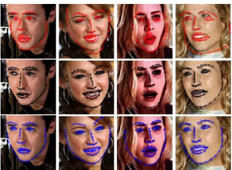
In this section, we propose a third orthogonal direction for employing AAMs in unconstrained conditions by means of training AAMs in-the-wild, and fitting using the proposed fast and robust algorithms (in particular, Fast-SIC, aFast-SIC and E-POIC). Interestingly, the combination of generative models plus training in-the-wild (plus robust optimization for model fitting) has not been thoroughly investigated in literature. It turns out that this combination is very benefi-cial for unconstrained AAM fitting. Consider for example the images shown in the first row of Fig. 1. These are test images from the LFPW data set. The images were not seen during training, but similar images of unconstrained nature were used to train the shape and appearance model of the AAM. The second row of Fig.1shows the reconstruction of the images from the appearance subspace. As we may see, the appearance model is powerful enough to reconstruct the texture almost perfectly. Because reconstruction is feasible, fitting an AAM to these images is also feasible if a robust algorithm is used for model fitting.

Fig. 1 First row:face images taken from the test set of LFPW (Belhumeur et al. 2011). The images were not seen during training.Second row: reconstruction of the images from the appearance subspace. The appearance subspace is powerful because the AAM was built in the wild

containing large variations in pose, illumination, expression and occlusion. For our experiments, in order to assess per-formance, we used the same average (computed over all 68 points) point-to-point Euclidean error normalized by the face size as the one used inZhu and Ramanan(2012). Similarly toZhu and Ramanan(2012), for this error measure, we pro-duced the cumulative curve corresponding to the percentage of test images for which the error was less than a specific value. In all cases, fitting was initialized by the bounding box ofZhu and Ramanan(2012).

Figure 2 shows the fitting performance of simultane-ous algorithms, namely Fast-SIC and aFast-SIC as well approximate project-out algorithms, namely E-POIC and

POIC. Figure3 shows some fitting examples. As we may

observe, Fast-SIC and aFast-SIC feature almost identical per-formance. As we can additionally observe from Fig.2, there is a large gap in performance between simultaneous algo-rithms (Fast-SIC and aFast-SIC) and POIC. However, this gap in performance is largely bridged by the proposed E-POIC which has the same complexity as E-POIC. In particular, we may observe that E-POIC-v1 performs comparably to E-POIC-v2, and they both outperform POIC by 10–20 % in fitting accuracy. Fortunately, the performance improve-ments achieved by E-POIC-v1 and E-POIC-v2 turn out to be orthogonal. As we may observe, the overall improvement achieved by E-POIC is almost equal to the summation of the performance improvements achieved by E-POIC-v1 and E-POIC-v2. As we additionally show in Sect.10, the perfor-mance gap between simultaneous algorithms and E-POIC is further reduced when one uses SIFT features to build the appearance model of the AAM.

8 Part-Based Active Appearance Models

In our formulation, a part-based AAM is an AAM that draws advantages from the part-based representation and the trans-lational motion model of the Deformable Part Model (DPM) (Felzenszwalb et al. 2010) and (Zhu and Ramanan 2012) (as opposed to the holistic representation and the piecewise

Fig. 2 Fitting performance ofpixel-basedAAMs on LPFW. Average pt-pt Euclidean error (normalized by the face size) versus fraction of images

affine warp used in standard AAMs). Following Tzimiropou-los and Pantic(2014), we call this model a generative DPM. As we show hereafter, fitting a generative DPM using Gauss– Newton optimization implies a translational motion model which results in more accurate and robust performance com-pared to that obtained by fitting a standard holistic AAM with the same algorithm. We attribute this performance improve-ment to the more flexible part-based representation which models only the most relevant parts of the face, and the sim-plicity of the translational motion model.

8.1 Generative DPM

Fig. 3 Fitting examples ofpixel-based AAMs from the test set of LFPW.First row:POIC.Second row:aFast-SIC.Third row:E-POIC. POIC does not perform well, however aFast-SIC and E-POIC achieved satisfactory robustness and accuracy in landmark localization. Notably, to obtain these results, the appearance model of the AAMs was built using raw un-normalized pixel intensities as features. Neither sophisti-cated shape priors or robust norms were used during fitting nor robust image features were employed to build the AAMs: we simply trained the AAMs in-the-wild on the same database

global shape model of the generative DPM is the same as the one used in AAMs, i.e. an instance of the shape model

s(p)is given by (1). A key feature of the appearance model is that it is learned from all parts jointly, and hence parts, although capture local appearance, are not assumed inde-pendent. The appearance model of the generative DPM is obtained by (a) warping each training imageIi to a

refer-ence frame so that similarity transformations are removed, (b) extracting aNp=Ns×Ns pixel-based part (i.e. patch)

around each landmark, (c) obtaining a part-based texture for the whole image by concatenating all parts in aN =u Np

vector, and (d) applying PCA to the part-based textures of all training images. In this way, and similarly to an AAM, we obtain the mean appearanceA0andmappearance eigenvec-torsAi, compactly represented as columns ofA∈ RN×m.

Again, and similarly to an AAM, an instance of the appear-ance modelA(c)is given by (2).

It is worth noting that eachAi(this also applies to the

part-based texture representation of each training imageIi) can be

re-arranged as au×Nprepresentation[Ai,1Ai,2 . . . Ai,Np].

Each columnAi,j ∈Rucontainsupixels all belonging to a different part but all sharing the same index locationjwithin their part. This representation allows us to interpret each patch as aNp-dimensional descriptor for the corresponding

landmark. Finally, we defineAj = [A1,j A2,j . . . Am,j] ∈

Ru_×m_.

8.2 Fitting Generative DPMs with Gauss–Newton

Similarly to an AAM, we can fit the generative DPM to a test image using non-linear least-squares optimization. We start by describing the fitting process of a simplified version of the generative DPM by assuming that the patch for each landmarkskis reduced to 1×1 (Ns =1), that is 1 pixel is used

to represent the appearance of each landmark and similarly the appearance model in (2) has a total ofN =u pixels. In this case, the construction of the appearance model, in the previous section, implicitly assumes a translational motion model in which each training image is sampled at N = u locationsIi(li)and thenu pixels are shifted to a common

reference frame which is defined as the frame of the mean shapes0. In this model, a model instanceMy is created by

first generatingu pixels using (2) for somec=cyand then

shifting these pixels tou pixel locations obtained from (1) for somep=py. Hence, we can write

My

s(py)

=A(cy). (21)

The above model can be readily used to locate the land-marks in an unseen imageIusing non-linear least-squares. In particular, we wish to find{p,c}such that

arg min

p,c ||I

s(p)−A(c)||2. (22)

Similarly to an AAM, the difference term in the above cost function is linear incbut non-linear inp. We therefore pro-ceed as in Sect.5and derive the same optimization problem as in (5) which, for convenience, we re-write here

arg min

Δp,Δc||I−A(c)−AΔc−JΔp||

2_,

(23)

where, for the case of the generative DPM, I = Is(p),

Ai =Ai(s(p=0)) =Ai(s0), andJi ∈ RN×nis the

Jaco-bian ofAi(notice thatN =u).

For the translational motion model defined above, we con-structJi as follows: Thek−th row ofJi contains the 1×n

vector[Ai,x(s0,k) Ai,y(s0,k)]∂s_∂k_p(p) |p=0.Ai,x andAi,y are

thex andygradients ofAi. To calculate ∂s_∂k_p(p) |p=0, let us

also denote bysk= [xk; yk]andsi,k= [x_ksi ; y_ksi]thek−th

landmark ofs(p)andsi, respectively. These are related by

sk =

xk; yk

=

x_ks0+

n

i=1 xsi

kpi ; y

s0

k + n

i=1 ysi

k pi . (24)

Finally, from (24), we have

∂sk(p) ∂p |p=0=

xs1

k . . .x

sn

k ; y

s1

k . . .y

sn

k

∈R2_×n_.

To optimize (23), one can use any of the algorithms

of Sects. 5 and 6. An interesting deviation from AAMs

though is that for the case of our translational motion model inverse composition is reduced to addition. To readily see this, let us first writesy = f(sx;pa) = sx +Spa. Then,

sz = f(sy;pb) = sy +Spb = sx + Spa +Spb =

sx +S(pa +pb), hence composition is reduced to

addi-tion. Similarly, we havef(sx;pa)−1= f(sx; −pa). Overall,

inverse composition is reduced to addition, and hencepcan be readily updated in an additive fashion fromp←p−Δp. Finally, having defined the 1-pixel version of our model, we can now readily move on to the case where the appearance of a landmark is represented by an Np = Ns ×Ns patch

(descriptor) each pixel (element) of which can be seen as a 1-pixel appearance model for the corresponding landmark. Using theAj representation defined in Sect. 8.1, the cost function to optimize for GN-DPMs is given by

arg min

Δp,Δc

Np

j=1

||Ij₋

Aj(c)−AjΔc−JjΔp||2. (26)

By re-arranging the terms above appropriately, it is not dif-ficult to re-write (26) as in (23) where now the error term

I−A(c)has sizeN =u Np, andJhas sizeN×n.

We repeated the experiment of Sect. 7 using the same number of shape and appearance parameters for the genera-tive DPM in order to evaluate all algorithms of Sects.5and6. The obtained results are shown in Fig.4. By comparing these results to those of Fig.2, we may observe that there is a gain of 10–20 % in fitting accuracy over AAMs. However, the relative difference in performance between all algorithms is similar. As we show later on, the performance gap between simultaneous algorithms and E-POIC is almost negligible when one uses SIFT features to build the appearance model of the generative DPM.

8.3 Comparison with AAMs

Two questions that naturally arise when comparing the part-based GN-DPMs over holistic AAMs are: (a) do both models have the same representational power? and (b) which model is easier to optimize? Because it is difficult to meaningfully compare the representational power of the models directly, in this section, we provide an attempt to shed some light on both questions by conducting an indirect comparison between the two models.

To investigate question (a), we repeated the experiment of Sect.7for both GN-DPMs and holistic AAMs, but we initial-ized both algorithms (we used Fast-SIC for both cases) using theground truthlocations of the landmarks for each image. We assume that the more powerful the appearance model is, the better it will reconstruct the appearance of an unseen

Fig. 4 Fitting performance of GN-DPMs on LPFW: Average pt-pt Euclidean error (normalized by the face size) versus fraction of images

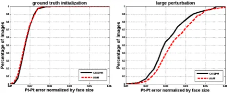
Fig. 5 Comparison between GN-DPMs and AAMs. Both algorithms were initialized using the ground truth landmark locations (left) and the ground truth after a relatively large perturbation of the first shape para-meter (right). The average (normalized) pt-pt Euclidean error versus fraction of images is plotted. Clearly GN-DPMs are easier to optimize

image, and hence the fitting process will not cause much drifting from the ground truth locations. Fig.5(left) shows the obtained cumulative curves for GN-DPMs and AAMs. We may see that both methods achieve literally the same fitting accuracy illustrating that the part-based and holistic approaches have the same representational power. An inter-esting observation is that the drift from ground truth is very small and the achieved fitting accuracy is very high. This shows that generative deformable models when trained in-the-wild are able to produce a very high degree of fitting accuracy.

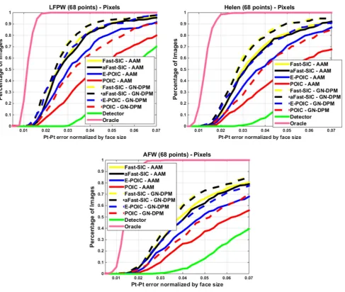
Fig. 6 Fitting performance ofpixel-basedAAMs and GN-DPMs on LFPW, Helen and AFW: Average pt-pt Euclidean error (normalized by the face size) versus fraction of images.68 pointswere used

9 Efficient Weighted Least-Squares Optimization

of SIFT-AAMs

All algorithms presented so far operate on raw pixel inten-sities. However, one could use other more sophisticated features to boost up robustness and accuracy. In this work, we used the same SIFT features asXiong and De la Torre(2013) which we found that they produce a large basin of attraction for gradient descent optimization. Building an AAM using SIFT features is straightforward. For example, for the case of standard holistic AAMs (for the case of GN-DPMs, the process is very similar) at each pixel location we extract a SIFT descriptor of dimensionNf, and the appearance of each

image is represented as a SIFT image (Liu et al. 2008) with Nf channelsIk,k = 1, . . . ,Nf. The appearance model of

the SIFT-AAM can be learned by warping eachIk_{to the mean}

shape, concatenating all features in a single vector and then applying PCA. In a similar fashion, the mean appearanceA0 and each appearance basisAican be rearranged inNf

chan-nelsAk_i,i = 1, . . . ,Nf. Finally for each appearance basis

and channel, we can calculate the JacobianJk_i as described in Sect.4.

Having defined the above notation, both holistic and part-based AAMs, and all algorithms presented so far can be readily extended for the case of SIFT-AAMs. For exam-ple, fitting a SIFT-AAM using the Fast-SIC algorithm entails solving the following optimization problem

arg min

Δp,Δc

Nf

k₌1

||Ik[p] −Ak₀−AkΔc−JkΔp||2_P

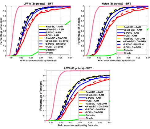
Fig. 7 Fitting performance ofSIFT-basedAAMs and GN-DPMs on LFPW, Helen and AFW: Average pt-pt Euclidean error (normalized by the face size) Vs fraction of images.68 pointswere used

Using robust features for building the appearance model of an AAM typically increases the complexity of the training, but more importantly, of the fitting process. If the descriptor has lengthNf, then the size of the appearance model isNfN,

and hence complexity increases by a factor ofNf. While we

used a reduced SIFT representation withNf =8 channels,

all resulting fitting algorithms are significantly slower (by a factor of 8) compared to their counterparts built from pixel intensities.

To compensate for this additional computational burden, we propose a fitting approach in which (3) is optimized over a sparse grid of points rather than all points belonging to the convex hull of the mean shape. In particular, this sparse grid is defined by aN ×N diagonal matrixWthe elements of which are equal to 1 corresponding to the locations that we wish to evaluate our cost function and 0 otherwise. UsingW,

we propose to formulate weighted least-squares problems for all algorithms proposed in this work. In particular, we write

arg min

Δp,Δc||I−A0−Ac−AΔc−JΔp)||

2

W. (28)

The question of interest now is whether one can come up with closed-form solutions forΔcandΔp. Fortunately, the answer is positive. Let us define matricesA_w = WA,

Ji,w = WJi, Jw = J0,w +

m

i=1ciJi,w, Pw = W −

Aw(AT_wAw)−1AT_w. Then, for Fast-SIC (similar update rules can be derived for all other algorithms described in this paper) we can updateΔcandΔpin alternating fashion from

Δc=AT_wA_w−1AT_w

WI−A(c)−J_wΔp

(29)

Δp=H−_w1_{f si c}JT_{wf si c}

whereJ_wf si c=P_wJ_w andH_wf si c =JT_{wf si c}J_wf si c,

respec-tively. Finally, notice that in practice, wenevercalculate and store matrix multiplications of the formWX, for any matrix

X∈ RN×l. Essentially, the effect of this multiplication is a reduced size matrix of dimensionN_w×l, whereN_w is the number of non-zero elements inW. In our implementation we used a grid such thatN_w/N =1/4. BecauseNf = 8,

the total cost of the algorithms is only increased by a factor of 2.

10 Results

We have performed a number of experiments in order to report a comprehensive evaluation of the proposed algo-rithms. We present results for3 Casesof interest:

Fig. 8 Convergence performance of SIFT-based AAMs and GN-DPMs on LPFW: Average pt-pt error versus iteration number

– Case 1: Evaluation of pixel-based AAMsWe have already assessed the performance of all algorithms presented so far for the popular data set of LPFW. To verify these results, we report fitting performance for two challenging cross-database experiments on Helen (Le et al. 2012) and AFW (Zhu and Ramanan 2012). We emphasize that the faces of these databases contain significantly more shape and appearance variation than those of the training set of LFPW that all methods were trained on.

– Case 2: Evaluation of SIFT-based AAMsWe report the fitting performance of the proposed algorithms when the appearance model was built using SIFT features for all three databases, and we focus on whether the proposed efficient weighted least-squares optimization of SIFT-based AAMs results in any loss in performance. – Case 3: Comparison with state-of-the-artWe present a

comparison on both human andanimalfaces between the performance of the proposed algorithms against that of two of the best performing methods in literature, namely the Supervised Descent Method (SDM) of (Xiong and De la Torre 2013) and Chehra (Asthana et al. 2014). We also compare the performance of all methods considered in our experiments against the best possible fitting result achieved by an Oracle who knows the location of the land-marks in the test images and simply reconstructs them using the trained shape model.

Below, we summarize 3 main conclusions drawn from our experiments:

– Conclusion 1aFast-SIC and Fast-SIC feature the same performance both in terms of fitting accuracy and speed of convergence.

Fig. 10 Comparison betweenSIFT-AAMsand SDM and Chehra on LFPW, Helen, AFW and our Cats data set: Average pt-pt Euclidean error (normalized by the face size) versus fraction of images.49 pointswere used for LFPW, Helen and AFW and42 pointswere used for the Cats data set

– Conclusion 2The part-based AAM (i.e. GN-DPM) built with SIFT features and fitted with E-POIC achieves essentially the same fitting accuracy as the same model fitted via aFast-SIC. To achieve this accuracy though, E-POIC requires about twice as many iterations. How-ever, the cost per iteration for E-POIC is orders of magnitude smaller than the cost per iteration required for aFast-SIC.

– Conclusion 3Our two best performing methods, namely GN-DPMs built with SIFT features and fitted with aFast-SIC and E-POIC, outperform SDM and Chehra. However, SDM and Chehra converge faster.

We now provide the details of our experiments: All AAMs, including holistic and part-based (GN-DPMs), and pixel-based and SIFT-pixel-based, were trained on LFPW as described in

Sect.7. Landmark annotations based on the Multipie config-uration for all databases (LFPW, Helen, AFW) are publicly available from the 300-W challenge (Sagonas et al. 2013). To fit all AAMs (both holistic and part-based), we used a multi-resolution approach with two levels. At the highest level the shape model has 15 shape eigenvectors and 400 appearance eigenvectors for all algorithms and AAMs. As for the sub-space of the steepest descent images used in E-POIC, we used 1200 and 2400 components for pixel-based and SIFT-based AAMs, respectively.

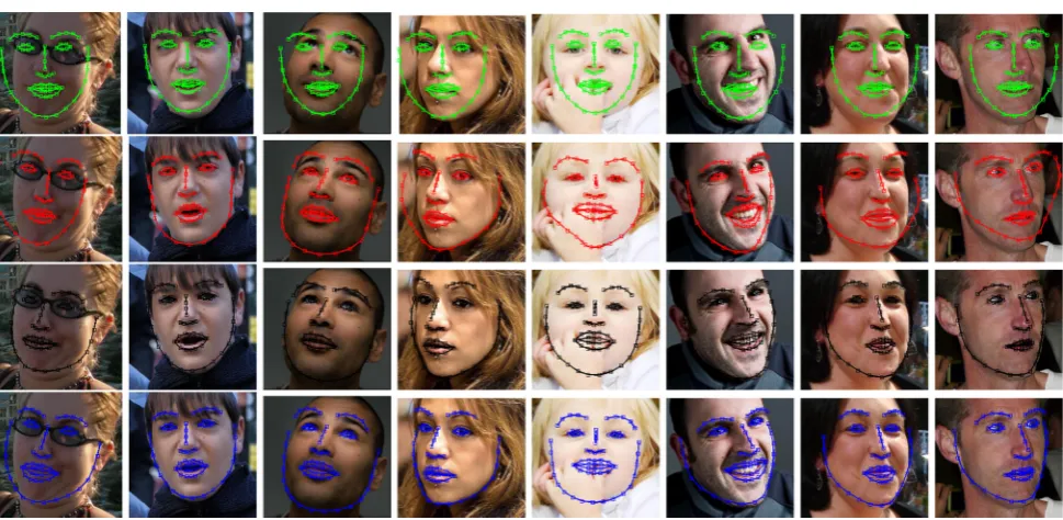
Fig. 11 Fitting examples ofSIFT-AAMsfrom Helen.First row:Detector.Second row:POIC-SIFT.Third row:aFast-SIC-SIFT.Fourth row: E-POIC-SIFT. aFast-SIC-SIFT and E-POIC-SIFT are significantly more robust and accurate than POIC-SIFT

the points of thesparse griddescribed in Sect.9. This setting is used for both AAMs and GN-DPMs. This means that if we exclude the cost for the SIFT extraction process, the aFast-SIC-SIFT, E-POIC-SIFT and POIC-SIFT algorithms have almost the same complexity as their pixel intensity coun-terparts (in particular the complexity is increased only by a factor of 2 as explained in Sect.9).

Similarly to the experiment of Sect.7, we initialized all algorithms using the bounding box of the face detector ofZhu and Ramanan(2012). To quantify performance, we produced the cumulative curves corresponding to the percentage of test images for which the normalized point-to-point error was less than a specific value. Note that forcases 1 and 2, we report performance for 68 points.

Regarding comparison with SDM and Chehra (case 3), we note that for the sake of a fair comparison we used the same implementation of SIFT that the authors ofXiong and De la Torre (2013) provide, although we used a reduced 8-dimensional SIFT representation as opposed to the 128-dimensional representation used inXiong and De la Torre (2013). As our experiments have shown, this reduced repre-sentation seems to suffice for good performance and keeps the complexity of SIFT-based AAMs close to that of their pixel-based counterparts. Probably, the good performance can be attributed to the generative appearance model of the AAMs which can account for appearance variation. Finally, we care-fully initialized both SDM and Chehra using the same face detector used for our AAMs, following the authors’ instruc-tions, and we report performance on the 49 interior points because these are the points that the publicly available imple-mentations of SDM and Chehra provide.

Figure6shows the results ofpixel-basedAAMs and GN-DPMs on Helen and AFW. Compared to LFPW, there is drop in performance for all methods because the faces of Helen and AFW are much more difficult to detect and fit. Nev-ertheless the relative difference in performance is similar, validating the conclusions of Sects.7and8.1. Notably, the part-based representation and the translational motion model of GN-DPMs consistently outperform the holistic appear-ance models and the piecewise affine warp of AAMs.

Figure7shows the results obtained by fittingSIFT-based AAMs and GN-DPMs on LFPW, Helen and AFW. We may observe that (a) there is large boost in performance when SIFT features are used, (b) there is negligible difference in performance between Fast-SIC-SIFT which is optimized overall pixels, and aFast-SIC-SIFT which is optimized on a sparse grid, (c) E-POIC-SIFT on a sparse grid largely outperforms POIC-SIFT, and performs almost similarly to aFast-SIC-SIFT. Especially for the case of GN-DPMs, the difference in performance between aFast-SIC-SIFT and E-POIC-SIFT is almost negligible.

convergence performance. This result clearly illustrates that, compared to Fast-SIC, the aFast-SIC approximation essen-tially achieves the same performance in terms of both fitting accuracy and speed of convergence. From the same figure, we can observe that E-POIC-SIFT requires almost twice as many iterations at the lower level compared to Fast-SIC-SIFT and aFast-SIC-Fast-SIC-SIFT. Hence, although E-POIC-Fast-SIC-SIFT achieves very similar fitting performance to that of aFast-SIC-SIFT (especially for GN-DPMs), it also requires more iterations. However, the cost per iteration for each algo-rithm is significantly different. After ignoring the feature extraction step, E-POIC requires one matrix multiplication to calculate the update for the shape parameters which on an average laptop takes about 0.0003 s. To perform the necessary matrix multiplications to calculate the update for the shape and appearance parameters, aFast-SIC is approximately 100 times slower, while Fast-SIC is approximately 5 times slower than aFAST-SIC. It is worth noting that E-POIC is very attrac-tive in terms of memory requirements as it requires storing

only one matrix of size N ×n in memory, while

aFast-SIC additionally requires storing the appearance model and its gradients. This makes E-POIC particularly suitable for mobile applications.

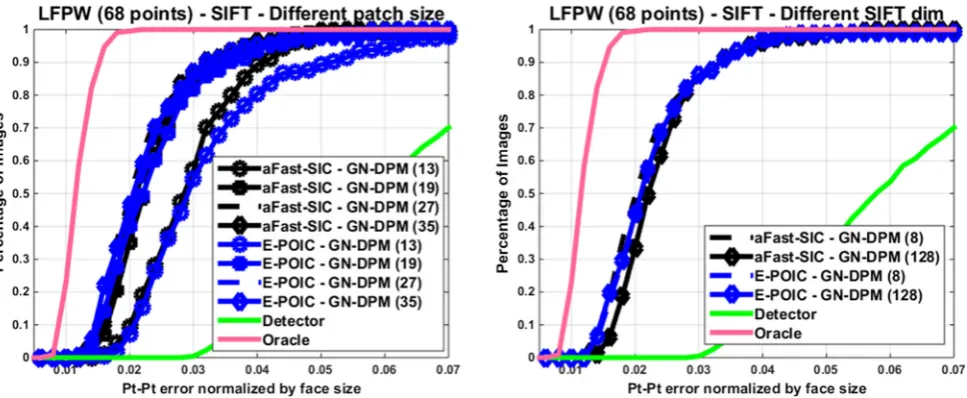
Figure9(a) shows the performance of our best performing GN-DPMs for different patch sizes Ns. It can be observed

that the method is not too sensitive to patch size and that performance starts saturating already fromNs =19. Figure

9(b) compares performance for SIFT dimensionality equal to 8 and 128. We observe that there is no benefit in increasing SIFT dimensionality (and hence complexity). We attribute this to the flexibility of the generative appearance model employed by AAMs.

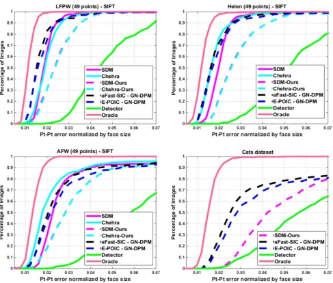
Figure10 shows the comparison between our two best

performing methods, namely GN-DPMs fitted via aFast-SIC-SIFT and E-POIC-aFast-SIC-SIFT and two state-of-the-art methods, namely SDM and Chehra. For this comparison, it is worth noting that we conducted experiments on human faces but also onanimal facesFor the former case, we followed our previous setting and trained aFast-SIC-SIFT and E-POIC-SIFT on about 800 images from LFPW. Note that SDM was trained on internal CMU data and Chehra on the whole LPFW, Helen and AFW data sets. As we may observe, the proposed methods outperform SDM on all three databases, and perform worse than Chehra only on the AFW data set. For the sake of a fairer comparison, we also provide the results of our implementation of SDM and Chehra, trained on LFPW. Finally, the later setting was repeated for our “Cats” data set which contains 1500 cat face images anotated with 42 land-marks (1000 images were used for training and 500 images for testing) selected from the Oxford pet data setParkhi et al. (2012). Because large pose variations and facial hair are very common in cat faces, this data set is much more challenging than the ones containing human faces. As we may observe,

compared to our implementations of SDM and Chehra, the proposed AAMs perform significantly better showing that AAMs can feature robust performance even when trained on relatively small data sets such as LFPW and very challenging data sets such as our “Cats” data set. We have to emphasize though that both SDM and Chehra require very few itera-tions to converge (about 5–6). Overall, these results clearly place the proposed methods in par with the state-of-the-art methods in face alignment. Finally, there is a very large per-formance gap between all methods and the best achievable result provided by the Oracle.

Finally, Fig.11shows some fitting examples of aFast-SIC-SIFT, E-POIC-aFast-SIC-SIFT, and POIC-SIFT on Helen. As we may observe aFast-SIC-SIFT and E-POIC-SIFT are significantly more robust and accurate than POIC-SIFT.

11 Conclusions

We presented a framework for fitting AAMs to unconstrained images. Our focus was on robustness, fitting accuracy and efficiency. Toward these goals, we introduced several orthog-onal contributions: First, we proposed a series of algorithms, perhaps the most notable of which are aFast-SIC-SIFT and more importantly E-POIC-SIFT. The former algorithm is rel-atively efficient, very accurate and very robust. The latter algorithm is very efficient, very accurate and, at the same time, notably robust. Secondly, we illustrated for the first time in literature the benefit of training AAMs in-the-wild. Thirdly, we introduced a part-based AAM combined with a translational motion model which is shown to largely out-perform the holistic AAM based on piece-wise affine warps. Finally, we introduced a weighted least-squares formulation for the efficient fitting of SIFT-based AAMs. Via a num-ber of experiments on the most popular unconstrained face databases (LPFW, Helen, AFW and Cats), we showed that E-POIC largely bridges the gap between exact and current approximate methods and performs comparably with state-of-the-art systems. Future work includes investigating how E-POIC can be extended for the case of regression-based techniques such as the one recently proposed in Tzimiropou-los(2015).

Acknowledgments The work of Georgios Tzimiropoulos was sup-ported in part by the EPSRC project EP/M02153X/1 Facial Deformable Models of Animals. The work of Maja Pantic was supported in part by the European Community Horizon 2020 [H2020/2014-2020] under grant agreement no. 645094 (SEWA).