The correlation between halo mass and stellar mass for the most massive galaxies in the universe

The Correlation between Halo Mass and Stellar Mass for the

Most Massive Galaxies in the Universe

Jeremy L. Tinker1, Joel R. Brownstein2, Hong Guo3, Alexie Leauthaud4, Claudia Maraston5, Karen Masters5, Antonio D. Montero-Dorta2, Daniel Thomas5, Rita Tojeiro6, Benjamin Weiner7, Idit Zehavi8, and Matthew D. Olmstead9

1

Center for Cosmology and Particle Physics, Department of Physics, New York University, New York, NY 10013, USA

2

Department of Physics and Astronomy, University of Utah, Salt Lake City, UT 84112, USA

3

Key Laboratory for Research in Galaxies and Cosmology, Shanghai Astronomical Observatory, Shanghai 200030, China

4

Kavli IPMU(WPI), UTIAS, The University of Tokyo, Kashiwa, Chiba 277-8583, Japan

5

ICG-University of Portsmouth, PO13FX Portsmouth, UK

6

School of Physics and Astronomy, University of St. Andrews, St. Andrews, KY16 9SS, UK

7

Steward Observatory, 933 N. Cherry Street, University of Arizona, Tucson, AZ 85721, USA

8

Department of Astronomy & CERCA, Case Western Reserve University, 10900 Euclid Avenue, Cleveland, OH 44106, USA

9

Department of Chemistry and Physics, King’s College, 133 North River Street, Wilkes Barre, PA 18711, USA

Received 2016 July 15; revised 2017 March 15; accepted 2017 March 19; published 2017 April 24

Abstract

We present measurements of the clustering of galaxies as a function of their stellar mass in the Baryon Oscillation Spectroscopic Survey. We compare the clustering of samples using 12 different methods for estimating stellar mass, isolating the method that has the smallest scatter atfixed halo mass. In this test, the stellar mass estimate with the smallest errors yields the highest amplitude of clustering atfixed number density. Wefind that the PCA stellar masses of Chen et al. clearly have the tightest correlation with halo mass. The PCA masses use the full galaxy spectrum, differentiating them from other estimates that only use optical photometric information. Using the PCA masses, we measure the large-scale bias as a function of M_* for galaxies with logM_*11.4, correcting for incompleteness at the low-mass end of our measurements. Using the abundance matching ansatz to connect dark matter halo mass to stellar mass, we construct theoretical models of b M( _*) that match the same stellar mass function but have different amounts of scatter in stellar mass atfixed halo mass,slogM_*. Using this approach, we

findslogM_*=0.18-+0.020.01. This value includes both intrinsic scatter as well as random errors in the stellar masses. To

partially remove the latter, we use repeated spectra to estimate statistical errors on the stellar masses, yielding an upper limit to the intrinsic scatter of 0.16 dex.

Key words:cosmology: observations –galaxies: abundances–galaxies: evolution –galaxies: halos–galaxies: luminosity function, mass function

1. Introduction

Galaxies are born, live, and die within dark matter halos. We have convincing evidence that the evolutionary history of galaxies and halos is correlated to a strong degree: brighter, bigger galaxies have higher clustering, indicative of being in more massive dark matter halos(see, e.g., Norberg et al.2002; Zehavi et al. 2005, 2011 for analyses at z~0; and Coil et al. 2006; Zheng et al. 2007; Wake et al. 2011; Leauthaud et al.2012at higher redshifts). Thus the growth of galaxies is related to the growth of dark matter halos. But how correlated are these two quantities? The purpose of this paper is to quantify this correlation by constraining the scatter in stellar mass atfixed halo mass for galaxies in the Baryon Oscillation Spectroscopic Survey (BOSS; Dawson et al. 2013). We will use two-point clustering as our probe of this scatter,slogM_*. For massive galaxies, clustering is an especially sensitive diag-nostic of the scatter, because it directly impacts their large-scale bias(e.g., Reddick et al.2013); more scatter means a sample of galaxies will contain a more significant sample of low-mass halos that will lower the overall clustering amplitude. BOSS galaxies specifically represent an excellent sample of highly biased objects, with previous small-scale measurements yield-ing clusteryield-ing amplitudes roughly four times higher than that of dark matter (White et al. 2011; Guo et al. 2013; Saito et al.2016).

However, unlike magnitude and color, galaxy stellar mass is not an observable. Different methods for derivingM_* produce different results. The scatter we constrain through clustering is the quadrature sum of the intrinsic scatter of stellar mass at

fixed halos,sint, and measurement error,serr. Different methods

of deriving stellar mass will have different serr but have the

same intrinsic scatter, since they are all estimates of the same physical quantity. Thus we can also use clustering to determine which method of obtaining stellar mass has the least variance. In this context, systematic offsets between codes or choices within codes, such as switching stellar initial mass functions, are immaterial. What we care about here is the rank-ordering of galaxies from most massive to least massive. Using clustering, we cannot probe systematic offsets between stellar mass estimates.

In addition to comparing different methods for determining stellar mass, we compare stellar mass with other physical properties of the galaxy. Specifically, Wake et al.(2012)used clustering to claim that stellar velocity dispersion, svel,

correlates better with halo mass than M_*. We will compare the clustering of galaxies ranked by 12 different variations of three different stellar mass codes, all of which are available in the public SDSS data releases, as well as two estimates ofsvel

and multiple galaxy luminosities.

2. Data

We use results from Data Release Ten of the Sloan Digital Sky Survey (Ahn et al. 2014). The spectroscopic footprint covers 6895 deg2 combined in the North Galactic Cap and South Galactic Cap regions, roughly 70% of the full BOSS footprint.

2.1. The CMASS Sample

The CMASS target sample is the workhorse of the BOSS large-scale structure analysis. Further details can be found in Dawson et al. (2013). These color cuts are meant to isolate massive galaxies at z0.4, but are somewhat more inclusive of blue galaxies than the traditional luminous red galaxy(LRG) sample from SDSS-II (Eisenstein et al. 2001). To limit the effects of the color cuts andflux limit of the survey, ourfiducial results are restricted to the range z=[0.45, 0.60], which surrounds the peak in the redshift distribution around 4 _´10-4 _(h-1_Mpc)3_.

The magnitudes used here are standard SDSS cmodel magnitudes, so-called because they are a composite of exponential and de Vaucouleurs profiles. In the SDSS pipeline, the profiles are truncated at three and seven times the scale radii for exponential and de Vaucouleurs profiles, respectively, smoothing going to zero at four and eight scale radii. See details in Abazajian et al. (2004). Due to the faintness of these targets, intracluster light (ICL) is typically below the surface brightness limits of observations. Also, as we will demonstrate in Section 4, the typical dark matter halo that houses a CMASS galaxy is_~1013M

, significantly below the

cluster mass regime. Behroozi et al. (2013a) estimate that, at

z~0.5, the ICL in 1013Mhalos is ~1 10 that of 1014Mhalos. The details of light profile fitting can have a

significant impact on the inferred stellar masses of CMASS galaxies, however. Bernardi et al. (2016)demonstrate that the Sérsic profilefits increase the magnitudes of the brightest end of the CMASS galaxy distribution, increasing the abundance of galaxies at M 1011.7M

*  relative to that derived using

cmodelmagnitudes. This would change our constraints on the stellar-to-halo mass relation(SHMR)at the very massive end— halo masses above _~1014M_{—but would not significantly}

change our constraints on slogM_*, because most of the constraining power on that quantity is at smaller galaxy masses. Additionally, the details of different light profilefitting does not impact the results we present in Section4.1, where we investigate the relative clustering amplitudes of various stellar mass estimates.

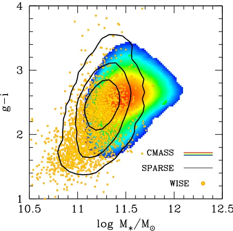
Figure1shows the mass versusg−icolor distribution for CMASS galaxies. We will describe the mass estimate used in thisfigure(PCA)in Section2.4. We useg−ibecause it more naturally separates blue and red galaxies at these masses and redshifts than other colors. Masters et al.(2011)demonstrates that a simple g- >i 2.35color cut best separates early type

and late type CMASS galaxies. At these redshifts,

g - =i 2.35 is similar to u- =r 2.22 at z=0, used by Strateva et al. (2001) to describe bimodality in the local universe. Unlike samples that probe galaxies near the knee in the stellar mass function(e.g., Blanton et al.2003), the CMASS sample is not bimodal in its colors. Although the color cuts are specifically designed to be more efficient at selecting passive objects than actively star-forming objects, the dominant factor in the lack of bimodality is simply that the CMASS selection is

targeting the very massive end of the galaxy distribution, with a median stellar mass ofM 1011.5M

*~ . At these masses, even

the SDSS Main sample exhibits no bimodality, but rather has a tail to bluer colors composed of the few star-forming objects at these mass scales. The CMASS selection is not devoid of any star-forming objects; Chen et al. (2012) find roughly 3% of CMASS objects at the median stellar mass have formed 10% of their stellar mass in the last Gyr.

2.2. The SPARSE Sample

The CMASS_SPARSE sample (hereafter SPARSE for

although the blue tail extends lower ing−ithan the CMASS sample.

The definition of the SPARSE sample has fluctuated somewhat over the course of the survey. In the first few months of observations, the color range was somewhat broader. We exclude these areas from consideration in the statistics, removing ∼140 deg2 of the overall footprint (delineated

“chunk2” in the BOSS order of observations; see Dawson et al.2013).

2.3. The WISE_COMPLETE Sample

Relaxing the color cuts even further than the SPARSE sample would dramatically reduce the efficiency of finding

z0.4galaxies. To efficiently locate galaxies in our desired redshift range, but outside the BOSS color cuts, ancillary data must be brought in. To this end, a series of 26 plates covering 59.8 deg2 were dedicated to observing three sets of ancillary targets, one of which was the WISE_COMPLETE target set. These targets incorporate data from the Wide-field Infrared Survey Explorer(WISE; Wright et al.2010). These targets have the same magnitude range as CMASS and SPARSE, but employ a single color cut,

r-W1>4.165, ( )1

to select galaxies in our desired stellar mass and redshift range that are outside the standard BOSS color cuts.10Here,W1 is the WISE3.4 micron band. Using WISE near-IR photometry is promising because the IR bands are on the far side of the peak of stellar emission, so an optical–IR color is sensitive to redshift. We will refer to the WISE_COMPLETE sample as WISEfor brevity.

There are 7368 objects within the WISEtarget catalog that receivedfibers and recovered accurate redshifts, 2200 of which are within the redshift range of interest. The g−i color distribution is broad and flat, with a median stellar mass of M 1011.06M

*= .

2.4. Physical Properties of the BOSS Galaxies

As discussed in the introduction, we are interested infinding the physical property that correlates the closest with halo mass via the clustering of the sample. We use stellar mass, galaxy luminosity, and galaxy velocity dispersion. Our main focus is stellar mass, but the question of whether stellar mass correlates any better with halo mass than does luminosity is still open. Table1shows all 16 variations of galaxy properties we use to rank-order the CMASS galaxy sample. Thefirst 12 are stellar masses that are included in the standard BOSS pipeline. There are three different codes for deriving stellar masses from BOSS data, with each code producing variants based upon parameter choices (i.e., stellar initial mass function, stellar population synthesis code, etc.).

The Portsmouth masses (Maraston et al. 2013) use two template star formation histories, one describes a passively evolving, old stellar population meant to mimic an LRG-type galaxy, and the other is an actively star-forming template. These two templates are combined to make one catalog: each galaxy is assigned a template based on its color, with a redshift-dependent break point of g- =i 3.25 +1.67(z-0.53). Galaxies redder than this color are assigned the passive template, with bluer galaxies assigned the star-forming template. Thus, although we list 14 different stellar mass definitions in Table1, there are only 12 different stellar mass catalogs, two of which are composed of the Portsmouth masses. The Granada masses are an implementation of the Flexible Stellar Population Synthesis (FSPS) mass modeling described in Conroy et al.(2009). The PCA masses(“principal component analysis”) are described in Chen et al. (2012). In contrast to the first two methods, the PCA approach uses the entire galaxy spectrum, decomposing it into principal compo-nents which are thenfit to a library of varying galaxy templates to obtain the physical properties of the galaxies, includingM/L ratio, velocity dispersion, and star formation rate. We note that theM/Lderived in the PCA method is theM/Lwithin thefiber aperture, which for BOSS is 2 arcsec. To obtain a total stellar mass, theM/Lratio is considered to be constant throughout the galaxy.

Table 1

Quantities to Rank-order the CMASS Galaxies

Number Property Code IMF Comments

1 Stellar mass PCA Kroupa BC03 SPS

2 Stellar mass PCA Kroupa M11 SPS

3 Stellar mass Granada Salpeter wide formation times, no dust

4 Stellar mass Granada Salpeter wide formation times, dust

5 Stellar mass Granada Salpeter early formation times, no dust

6 Stellar mass Granada Salpeter early formation times, dust

7 Stellar mass Granada Kroupa wide formation times, no dust

8 Stellar mass Granada Kroupa wide formation times, dust

9 Stellar mass Granada Kroupa early formation times, no dust

10 Stellar mass Granada Kroupa early formation times, dust

11 Stellar mass Portsmouth Kroupa SF template

12 Stellar mass Portsmouth Salpeter SF template

13 Stellar mass Portsmouth Kroupa passive template

14 Stellar mass Portsmouth Salpeter passive template

15 Luminosity L L absolute,i-band

16 Luminosity L L absolute,i-band,k-corrected

17 Velocity dispersion PCA L L

18 Velocity dispersion Portsmouth L L

10

We use two different estimates of the stellar velocity dispersion, one that is produced by the PCA analysis, the other produced by the Portsmouth analysis code(see details for the latter in Thomas et al.2013). Lastly, we use absolutei-band magnitude as our baselines rank-order by which to compare all the methods. We also include a sample that has been k-corrected toz=0.52 using thekcorrectcode of Blanton & Roweis(2007).

3. Measurements

3.1. The Completeness and Abundance of the BOSS Galaxy Samples

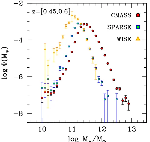
Figure2shows the stellar mass function,F(logM_*), for each of the three samples discussed previously. All results use the PCA stellar masses. We estimateF(logM_*)using the1 Vmax method,

while noting that theVmax weighting really only effects the results

at stellar masses below the peak of each distribution. The main source of incompleteness in these measurements is the color selection imposed on each sample. The CMASS sample dominates the statistics at high masses, but the combination of the SPARSE and WISE samples becomes equivalent to the CMASS abundance atlogM_*~11.4.

We use the abundance of SPARSE and WISE galaxies to quantify the completeness of the BOSS target selection. Figure 3 shows the ratio of the CMASS SMF to that of the total SMF (i.e., CMASS+SPARSE+WISE) as a function of

M

log _*. The CMASS sample is roughly 50% complete in stellar mass at logM_*=11.4. These results are in reasonable agreement with those of Leauthaud et al. (2016), which uses the extra near-infrared imaging data available in Stripe 82 to estimate completeness. Although the combination ofWISEand SPARSE data get us most of the way to a fully complete

sample, the total sample used in this paper is still missing 10%

~ of galaxies at logM=11.4. The stellar masses of Leauthaud et al.(2016)are different than the PCA masses used here, due to the inclusion of infrared imaging data. From the comparison between the near-IR masses and the PCA Bundy et al.(2015), there is a shift of 0.15 dex between the two mass definitions, which we use to shift the Leauthaud et al. (2016)

completeness curves onto the PCA mass scale.

AtlogM_*=11.4, the combination of CMASS and SPARSE is roughly 75% complete. Henceforth we will limit all analyses to be above this mass scale. The limited size of the WISE sample prevents us from making robust clustering measure-ments forWISEgalaxies; thus we make the assumption that the bias ofWISEgalaxies and SPARSE galaxies is the same when combining the clustering results of the samples. This does not significantly affect our results; the constraining power onslogM_* derives from the region of the SMF, where CMASS dominates the statistics.

Figure4shows the completeness-corrected SMF of massive galaxies down to the limit oflogM_*=11.4. Wefit these data using afitting function of the form:

M M

M

M M

1 ln 10 , 2

1 1

1

* * * *

F = F +

a b g a b

+

-⎛ ⎝

⎜ ⎞

⎠

⎟ ⎡

⎣ ⎢ ⎢

⎛ ⎝

⎜ ⎞

⎠ ⎟ ⎤

⎦ ⎥ ⎥

( ) ( ) ( )

( ) ( )

with best-fit parameter values of _{F =*} 2.43_´10-2_,

M

log 1=11.47,a=0.728,b =1.173, andg= -6.01. This

fitting function will be used to map galaxy mass onto halo mass using the abundance matching method in Section4.3.

3.2. Measuring Clustering

Our statistical measure of the clustering of galaxies within BOSS is the projected two-point correlation function w rp( )p . Figure 2.Comparison of the space densities of each individual BOSS targets

class. All measurements implement atVmax correction, which has minimal

effect atlogM_*11.4but can significantly enhance the measured abundance at low masses. Red circles represent the CMASS targets. Green squares represent the SPARSE sample. Yellow triangles represent theWISEdata. Each of these measurements peaks at a lower stellar mass, demonstrating the effect of reaching further outside the typical LRG color selection.

This statistic integrates the two-dimensional redshift-space correlation function,x(rp,rp), along the line-of-sight direction

r_π.w rp( )p is defined as

w rp p 2 rp,r dr, 3

0

max

ò

= ´ p p p

( ) ( ) ( )

where rpis the projected separation between galaxy pairs and

max

p is the maximal line-of-sight separation, which here we make 80h-1Mpc_{. To estimate r,r}

p

x( p), we use the Lansy– Szalay estimator (Landy & Szalay 1993) with 107 randoms. Whenpmax= ¥, the projected correlation function is identical

whether the argument in the integrand is the real- or redshift-space correlation function. Having a finite pmax introduces

some deviation from a real-space-only calculation (see, e.g., van den Bosch et al.2013).

The projected clustering of galaxies is our preferred statistic for two reasons. First, peculiar motions are(mostly)removed in the line-of-sight integration. At large scales there is still a residual effect, but we will model this out whenfitting for bias. Second, in the third paper in this series, we will present halo occupationfits of the clustering to determine the stellar-to-halo mass ratio of BOSS galaxies. Removing the peculiar motions makes such modeling less cosmologically dependent and easier to implement analytically.

To estimate the errors on the correlation function, we jackknife the DR10 footprint into 100 roughly equal-size angular regions, removing one subsample at a time and calculating the covariance matrix as

C N

N w w w w

1

, 4

ij

n N

i i j j

1

å

= - -

-=

( ¯ )( ¯ ) ( )

where N is the total number of jackknife subsamples (100),i and jrepresentrpbins, andw¯ represents the mean correlation

function in each bin.

To correct for fiber collisions, we use the angular-upweighting method as described in White et al. (2011). On a given plate,fibers can only be positioned within 62 arcsec of one another. Atz=0.5, this translates to a projected separation of about 400 kpc/h. Roughly 40% of the area within the survey is covered by multiple plates. These areas have nearly unit completeness, at least in terms of fiber assignment. Galaxy pairs within the collision radius are upweighted by the ratio of the angular correlation function of all CMASS targets, to those for which fibers were assigned at the angle of the pair in question. Inside 62″, this ratio11 is nearly a constant value of 2.57. In practice, we only use this method to correct for onerp

bin inside the collision radius, and for no bins that effect our bias calculation.

We measure the autocorrelation of the CMASS sample, but the SPARSE sample, by definition, has too low a density to make a robust measurement of the clustering. We thus cross-correlate the SPARSE and CMASS samples to get the relative bias between these two samples, and then divide by the bias of the overall CMASS sample, which is 1.99±0.04 for the cosmology chosen.

3.3. Measuring Bias

We use the projected separation range5<rp<35h-1Mpc to determine the bias relative to the clustering of matter. Although clustering is more linear at larger scales, errors on clustering rise monotonically with scale. Additionally, as rp

increases, the contribution of peculiar velocities tow rp( )p also monotonically increases. Although we model out the peculiar motions, the optimal approach is to extend therprange out as

far into the linear regime as possible, while keeping the effect of afinitepmax to under 25%.

To recover linear bias from our clustering measurements, we need to model both peculiar velocities and nonlinear clustering. Rather than try to subtract these effects out of our measure-ments, we add them into the model for the matter clustering. First we model real-space galaxy clustering as

r b m r r , 5

gal gal 2

x ( )= x ( ) ( )z ( )

wherex_m( )r is the nonlinear matter correlation function from Smith et al. (2003), bgal is the bias parameter for the galaxy

sample, andz( )r is the scale-dependent halo bias function from Equation(B7)in Tinker et al.(2005). This scale-dependence of halo bias, relative to the large-scale value, asymptotes to unity at r20h-1Mpc_{, with a maximum deviation of ~10% at}

r~2h-1Mpc _{(see Figure 12 in White et al.2011 for a halo} occupation fit of the scale-dependent bias of BOSS CMASS galaxies). At smaller scales, the scale-dependence of galaxy bias becomes dependent on the details of halo occupation, and it is only partially correlated with bias at large scales.

Second, we incorporate the effects of peculiar velocities using the linear approximation of Kaiser (1987). Although peculiar velocities are poorly described by linear theory at

r20h-1Mpc_,

max

p of 80h-1Mpc _{eliminates the} contrib-ution of redshift-space distortions at scales where linear theory breaks down. The configuration-space implementation of the Kaiser effect is described in detail in Appendix A of Hawkins et al.(2003).

Figure 4. Upper panel: the total BOSS stellar mass function at

z=[0.45, 0.60], down to our completeness limit of logM_*=11.4. The best-fit parameters of equation(x)are shown with the solid curve. Lower panel: residuals of thefit. They-axis is(FBOSS- Ffit) Ffit. Thec2for thisfit is 7.0

for(10–5)degrees of freedom.

11

In practice, wefit forbgalbyc2 minimization using the full

covariance matrix.

3.4. Numerical Simulations

Our theoretical models are created using the publicly available halo catalog from the MultiDark simulation (Nuza et al. 2013). The cosmology for this simulation isW =m 0.27 and s8=0.82. The halo catalog incorporates halos and subhalos using the ROCKSTAR algorithm of Behroozi et al. (2013b). We populate these halos with galaxies, using the subhalo abundance matching model (a.k.a. SHAM; see Reddick et al. 2013 and references therein). In its simplest form, abundance matching provides a unique mapping of halo mass onto galaxy mass(or galaxy luminosity) by assuming a one-to-one relation between the two without any scatter. There are multiple ways to incorporate scatter(Behroozi et al.2010; Trujillo-Gomez et al. 2011). We use the method in Wetzel & White (2010), in which the stellar mass function is first deconvolve of lognormal scatter of widthslogM_*. This allows us to employ the simple abundance matching method using the monotonic relation between M_* and Mh. Then thelogM_* of

each galaxy is shifted by a random Gaussian deviate of the same width.

Once halos are populated with galaxies, the large-scale bias of the model is calculated by binning the mock galaxies by

M

log _*in the same manner as the data, and summing over each halo in the stellar mass bin, weighting each galaxy by the bias valueb Mh( halo)given by the Tinker et al.(2010)bias function.

For subhalos, we use the mass of the host halo(the halo that the subhalo is located within)to calculate the bias. More explicitly, the bias of sample galaxies is given by summing over each galaxy, i, in the sample,

b

N b M

1

, 6

i

h i

gal gal

host

å

= ( ( ) ) ( )

where Ngal is the total number of galaxies in the sample. This

approach allows us to calculate the large-scale bias rapidly,

without explicitly measuring the clustering of the mock galaxies. This is also less noisy than measuring the clustering, an important feature in this method, as the BOSS data is actually a larger volume than the MultiDark simulation.

4. Results

4.1. What Galaxy Property Correlates Most with Halo Mass?

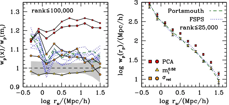
Figure5compares the clustering of all 18 properties listed in Table1 atfixed number density. For each quantity, we rank-order the sample form highest to lowest value. In this method, cutting the samples at a given rank means that each sample has the same number density. In the left panel, we show w rp( )p relative to thei-band w rp( )p for the top 100,000 galaxies for each property(about~1 3the total sample). In the right panel, we show the results for the top 25,000 galaxies in each property, although in the right panel we only show a subset of the properties considered. These two sample sizes correspond roughly to the number densities of _~1.2_´10-4 _and

h

0.3_´10-4₍ -1Mpc₎-3_{, respectively.}

The left panel demonstrates that the observed scatter between halo mass and luminosity is larger than all other galaxy properties considered, regardless of the stellar mass code employed. The cabal of photometrically based stellar mass estimates yield a bias roughly 3% higher than i-band magnitude. Because all the different variations of these two codes are roughly consistent with one another, we do not attempt to differentiate them in the plot. The clustering for these samples increases sharply atrp<1h-1Mpcrelative to i-band clustering. Clustering at these scales is reflective of the number of satellite galaxies per halo (often referred to as the

sample. For the CMASS target selection, which preferentially selects red galaxies, the impact of this argument is less clear. However, the increase in the clustering in one-halo terms argues that the small fraction of blue galaxies in CMASS is coming into play when rank-ordering the same by luminosity and by stellar mass.

The amplitude of clustering for the samples defined by velocity dispersion is consistent with the photometrically derived stellar masses. For some photometric stellar mass codes, the clustering of the velocity dispersion sample is slightly higher than the photometric stellar mass clustering, but when considering the entire ensemble of photometric mass definitions, it is not clear that there is any differentiation between the two properties when it comes to clustering amplitude.

The spectroscopic PCA masses have a clustering amplitude 25%

~ higher than i-band clustering, significantly higher than both velocity dispersion and photometric stellar mass. Although we do not perform any halo occupation fits of the clustering, it is improbable to ascribe the boost in the large-scale amplitude entirely to an increase in satellite galaxies; as opposed to the photometric stellar masses, the relative w rp( )p for the PCA masses decreases in the one-halo term. In the right panel, we restrict the lists to only the highest 25,000 objects by rank. In this sample, the difference between the PCA clustering and the other samples is large enough—∼60%—to be seen clearly on a logarithmic scale, and without taking ratios. In this panel, we show only a subset of clustering results in order to avoid crowding of the plot.

We note that the enhanced clustering of the PCA masses is not due to any selection effect (i.e., in the samples in the left and right panels of Figure 5, the distribution of color and luminosity for the most massive PCA galaxies are nearly indistinguishable from the most massive FSPS and Portsmouth galaxies). We therefore conclude thatslogM_*, and by extension

err

s , for the PCA masses is smaller than for photometrically defined stellar masses, galaxy luminosity, and stellar velocity dispersion. For the remainder of this paper, all results will use the PCA masses with the BC03 SPS code.

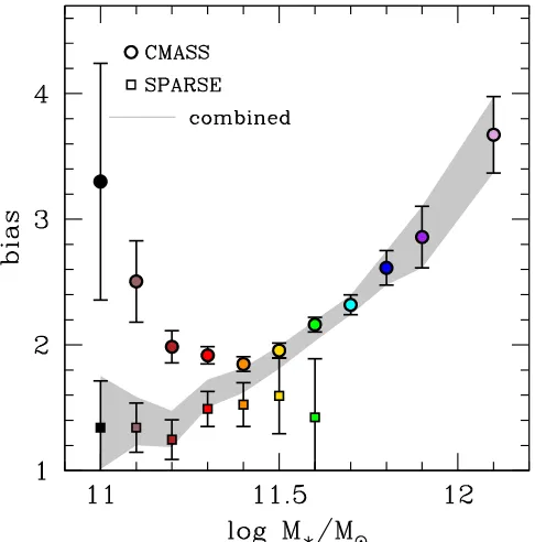
4.2. Bias as a Function of Stellar Mass

Figure6 shows the measured values ofw rp( )p for CMASS and the total CMASS sample crossed with SPARSE galaxies, binned by stellar mass. Using the technique described in Section3.3, wefit forbgalfor each bin inM_*for CMASS and

for the CMASS-SPARSE cross-correlation. Figure7shows the results for each sample. The SPARSE results have had the bias of the overall CMASS sample divided out. AtlogM_*11.4, the CMASS bias rises monotonically with stellar mass. Not coincidentally, this is the mass range where the CMASS sample is most complete in stellar mass. In terms of space density, the CMASS sample peaks at logM_*=11.4, and rapidly decreases at smaller masses, mainly due to the color Figure 6.Left panel: projected clustering of CMASS galaxies binned by stellar mass above the completeness limit of the CMASS selection algorithm. The solid black curve shows the nonlinear clustering of dark matter. Middle panel: clustering of CMASS galaxies at and below the completeness limit of the sample. Right panel: cross-correlation function of the SPARSE sample, binned by stellar mass, with the full CMASS sample. In each panel, the numbers on the right side indicate the center of the bin inlogM_*.

cuts. At logM_*<11.4, the CMASS bias rises back up again. This rise at low masses can be explained if the target selection cuts preferentially select satellite galaxies at lower masses. Previous studies of color-dependent clustering have shown this U-shaped behavior is red galaxy clustering(see, e.g., Swanson et al. 2008; Ross et al. 2011), a trend that is driven by the increasing fraction of satellite galaxies in the red subsample as luminosity or stellar mass decreases. In contrast to those results, the minimum bias shown in Figure 7 is at a much higher mass relative to the knee in the stellar mass function, but it is possible that the effect is amplified by the BOSS CMASS color cuts.

However, the clustering of the SPARSE sample is nearly independent of stellar mass. The WISE sample is not large enough to afford spatial clustering analysis, so we make the approximation that the WISEclustering is the same as the SPARSE and weight the SPARSE clustering results accord-ingly. The shaded band represents the total bias of galaxies in the combined sample weighted by the relative number of the CMASS versus the (WISE+SPARSE)samples.

4.3. Scatter of Stellar Mass at Fixed Halo Mass

Figure8 compares our combined bias results to predictions from the numerical simulation described in Section 3.4. As described previously, each curve represents a model that matches the same stellar mass function, but has different amounts of scatter between halo mass and stellar mass. Four different curves representing differentslogM_*values are shown for comparison. A model with zero scatter would predict clustering too high relative to the results. A model with scatter atslogM_*=0.26is ruled out because the clustering amplitudes are too low. The best-fit value ofslogM_* is 0.18, with a 68% confidence interval of[0.16, 0.19].

The SDSS pipeline reports a mean error of 0.16 dex for the PCA masses. This includes both systematic and random errors. To estimateserr—the statistical errors alone—we use repeated

spectra of CMASS galaxies that occur on regions of the footprint covered by multiple tiles. The rms difference in masses between the repeat spectra is 0.11 dex, implying that the intrinsic scatter of stellar mass atfixed Mhalo is 0.16 dex.

The completeness at M 1011.5

* deviates from unity, so it is

possible that slogM_* of galaxies that pass the CMASS and SPARSE color cuts is not representative of the full scatter, but it is clear that the bias at these masses is relatively insensitive to

M

log _*

s and the constraints are driven by the higher masses.

4.4. The Stellar-to-halo Mass Relation

Figure9shows the SHMR using the best-fitslogM_*value of 0.18. The solid curve represents the mean stellar mass atfixed halo mass,áM M_*∣ haloñ. Due to the steepness of the halo mass

function, the reverse relation,áMhalo∣M_*ñ, is quite different. The filled circles show theáMhalo∣M_*ñfor the bins analyzed in this

paper. The errors show the inner 68% of the distribution of

M

log halo in each bin, demonstrating the significant overlap in

the halo distribution analyzed in each bin.

The left side of Figure10shows the sensitivity of the SHMR to the assumed value ofslogM_*. AtslogM_*=0.13, the SHMR is a steeply rising function of Mhalo. At slogM_*=0.20, M_* becomes nearly independent of halo mass at logMhalo14. The reverse relation,áMhalo∣M_*ñ, shows the opposite trend: as

M

log _*

s gets larger, the mean halo mass atfixed M_*decreases, yielding the trend of the theoretical models in Figure 8 and producing the tight constraints onslogM_*.

The right side of Figure10compares our best-fit relation to a sample of other measurements. Those based purely on abundance matching—that is, where no other data other than the stellar mass function is fit (Behroozi et al. 2013a and Moster et al. 2013 in the figure)—lie significantly below our Figure 8. The combined CMASS+SPARSE bias values compared with

models derived by abundance matching dark matter halos and subhalos in the MultiDark simulation and the stellar mass function of BOSS. Different curves indicate different values of scatter(inlogM_*)in stellar mass atfixed halo mass.

Figure 9. The stellar-to-halo mass relation (SHMR) for BOSS CMASS galaxies using the PCA stellar mass estimates. The solid green curve shows the meanM_*in bins ofMhalo, with the dashed curves indicating the 0.18 dex in

scatter of the best-fit relation. The colored circles show the meanMhaloin the

observed bins inM_*used in this paper. Error bars indicate the inner 68% of the distribution oflogMhaloin each bin. The gray shaded region indicates the

relation. This comparison is complicated by different stellar mass estimates and significantly smaller data samples atz=1, but it is clear the estimates that probe this relation directly using galaxy groups and clusters are in better agreement with the BOSS relation (Lin & Mohr 2004; Hansen et al.2009; Yang et al. 2009,2012). Finally, our results are in good agreement with the SHMR for BOSS galaxies obtained by Rodríguez-Torres et al. (2016). This relation is based on the Portsmouth stellar masses(line 13 in Table1), and the abundance matching is based on peak circular velocity, with a scatter of0.31´Vpeak

obtained by matching the redshift-space monopole of the galaxy correlation function.

5. Discussion

In this paper we have demonstrated a novel method of discriminating between disparate methods of estimating the stellar masses of galaxies. We caution that the clustering results represent only half the story when it comes to appraising different methods, because clustering is only sensitive to the rank-ordering of a set of galaxies, from most massive to least massive, which in turn provides information on the scatter induced in the estimation of M_*. However, the method has nothing to say about absolute offsets between different methods. Using this technique, the stellar masses derived from the PCA code of Chen et al. (2012) correlate more strongly with halo mass thani-band magnitude, velocity dispersion, and other estimates of stellar mass provided in the BOSS pipeline. These other stellar masses are based on photometric data only, while the PCA masses are based on analysis of the spectral information. The PCA method has the limitation that the spectra only contain information about the galaxy from within the diameter of thefiber, which for BOSS is2. This may lead to aperture bias for the derived quantities, but any bias goes in the direction of strengthening the correlation with halo mass, which indicates something fundamental about the quantities being estimated. But given the average radius of the typical BOSS galaxy of 1 2(Masters et al.2010), aperture bias might

be non-negligible, but it is unlikely to be the dominant source of the differences between the methods.

Bundy et al. (2015) present a detailed comparison of the Porstmouth and PCA masses, with masses obtained using extra-infrared imaging available in the SDSS southern equatorial stripe, “Stripe 82” in the collaboration parlance. The dispersion between the Portsmouth masses12and the near-IR masses is 0.29 dex, while the dispersion between near-near-IR and PCA masses is 0.20. The tighter correlation with near-IR masses supports the results here that the PCA masses have a smaller intrinsic scatter relative to other photometric-based methods.

However, as discussed previously, there is a bias between the near-IR and PCA of 0.15 dex as well, as well as an offset of the PCA masses with respect to the Porstmouth values(Chen et al. 2012). Additionally, the lower amplitude of the PCA

w rp( )p atrp<1Mpch−1is indicative of fewer satellite galaxies in the PCA sample relative to the other stellar mass samples(cf. Figure5). This does not mean that satellites are“missing”from the PCA catalog, but rather that they are assigned lower masses than in other catalogs. Satellites should be redder than the overall population, implying that the PCA methodfinds higher stellar masses for bluer galaxies relative to other methods. Tinker et al.(2012)found that X-ray groups with bluer central galaxies have higher clustering atfixed halo mass, at the same redshift and stellar mass as the BOSS sample. Tinker et al. (2012) concluded that this was assembly bias in massive galaxies, with the caveat that the sample was statistically limited. It is possible that the higher clustering amplitude of the PCA masses is partly due to an assembly bias effect imparted by the relative ranking of bluer and redder galaxies within the catalog, and not entirely from a minimization of intrinsic scatter. The evidence for this is circumstantial at best, but is worth further investigation.

Figure 10.Left side: the sensitivity of the SHMR to the assumed value ofslogM_*. The solid curves show the SHMR for each value of scatter indicated in the key. The

dashed curves show the meanMhaloin bins ofM_*. Thisfigure explains why the bias in Figure8,b M( _*), decreases as the scatter increases. Right side: comparison of

the SHMR derived here to other measurements in the literature. There are few measurements atz=0.5, so we show values atz=0 andz=1 from the same works, with the expectation that thez=0.5 value should lie somewhere in between. Estimates of the SHMR from abundance matching, such as Behroozi et al.(2013a)and Moster et al.(2013), lie significantly below the relation here. Values derived from cluster samples appear to be in much better agreement with BOSS. Lastly, we are in good agreement with the results of Rodríguez-Torres et al.(2016), who also analyze the CMASS sample but using a different stellar mass estimate and abundance

matching technique.

12

The Portsmouth masses used here, which are a combination of the two templates based on galaxy color, are referred to in Bundy et al. (2015) as

It is noteworthy that all stellar mass estimates considered here correlate with halo mass better than absolute magnitude. The CMASS sample, although it is primarily intended to target luminous red galaxies, does have a non-negligible component of star formation galaxies with blue(ish) colors that have a lower clustering amplitude at fixed Mi(Guo et al.2013). We

conclude that almost any estimate of stellar mass provides a more robust rank-ordering of a heterogeneous color sample of galaxies relative to luminosity alone.

In our analysis, the photometric stellar mass indicators provide the same level of scatter as velocity dispersion, all of which yield a larger scatter than the PCA stellar masses. Wake et al. (2012)used clustering to claim that velocity dispersion had a stronger correlation with halo mass than stellar mass, a result that was challenged by Li et al.(2013), who claim that the Wake etal.result is contaminated by satellite galaxies, and once these satellites are removed, stellar mass has the strongest correlation. Our results suggest that the choice of stellar mass estimator can play a large role in this comparison. Both Wake etal.and Li etal.employ photometric mass estimates, which are likely to include extra measurement scatter, although we do not test their exact methods. We make no attempt to remove satellite galaxies from our analysis, but the satellite fraction of BOSS galaxies is low (fsat =0.100.02 from White et al.2011), and it is clear in Figure5that the PCA clustering in the one-halo term (rp1 Mpch-1)is lower relative to the

photometrically based codes. This implies that the satellite fraction of the PCA sample is smaller than the satellite fraction of the other samples, thus not artificially enhancing the clustering of the sample. Our theoretical modeling includes subhalos in the abundance matching procedure, and this method yields the proper satellite fraction of BOSS galaxies (Nuza et al.2013).

Our constraint onslogM_*of0.18 0.02 0.01

-+

compares favorably with other estimates from the literature. Zu & Mandelbaum(2016)use abundance and lensing data to obtain slogM_*=0.200.01 at

Mhalo=1013h-1M(linearly interpolating between their results

at 1012and 1014). More et al.(2011), using satellite kinematics,

find 68% confidence regions of[0.14, 0.21]for red galaxies and 0.07, 0.26

[ ]for blue galaxies in the SDSS Main sample. Reddick et al. (2013), using the SHAM approach with multiple free parameters constrained by both clustering and comparison to an SDSS group catalog, find slogM_*=0.200.03. Leauthaud et al.(2012)apply the SHMR approach to multiple statistics in the COSMOSfield tofindslogM_*=0.250.02at similar redshifts to those probed here. Our constraint has both the smallest uncertainty and the lowest value itself. The previous measure-ments used photometrically derived stellar masses, which must be contributing to the measurement scatter in each study. Kravtsov et al.(2014)measure the scatter in brightest cluster galaxy mass for a sample of X-ray clusters, findingslogM_*=0.170.02, which is in excellent agreement with our results. The notable aspect of the comparison between Kravtsov et al.(2014)and our results is that they are largely distinct in the halo masses probed. Kravtsov etal.analyze clusters atMhalo1014h-1M, which is

the upper limit of the halo masses probed by out stellar mass bins. This implies that slogM_* is independent of halo mass over the range12.7logMhalo15.2. This has largely been assumed, mainly because existing data could befit with a constant scatter, and constraints onslogM_*at low halo and galaxy masses are very weak because of the lack of variation of bias with halo mass at those scales. Additionally, all of these results imply little to no

redshift evolution inslogM_*for massive galaxies. This is expected, given that the maority of the galaxy population at these masses is passively evolving, although strict passive evolution does notfit the evolution of the clustering of massive galaxies over the same timespan(Zhai et al.2016).

Gu et al.(2016)investigate the origin of scatter atfixed halo mass by following the hierarchical buildup of both dark and stellar mass in simulations using abundance matching as a function of cosmic time. They find thatslogM_* from merging alone(e.g.,“ex-situ”stellar mass growth)can account for 0.16 dex of scatter at cluster-scale halo masses. This is in excellent agreement with Kravtsov et al.(2014), but the comparison with the BOSS results is more nuanced. Our SHMR indicates that the average 1014h-1M

halo contains at1011.5Mgalaxy, but

once binned by stellar mass, the average halo at that mass scale is_~1013_h-1_M

. The Gu et al.(2016)simulations indicate that,

at that halo mass,“in situ”processes dominate. The abundance matching analyses indicate that the fraction of stellar mass from merging for Mhalo~1013h-1M is low,10% from Moster

et al. (2013) and 25% from Behroozi et al. (2013a). Thus CMASS galaxies, although they are among the most massive in the universe, still are a sensitive probe of the physics of galaxy formation.

I.Z. is supported by NSF grant AST-1612085. Funding for the Sloan Digital Sky Survey IV has been provided by the Alfred P. Sloan Foundation, the U.S. Department of Energy Office of Science, and the Participating Institutions. SDSS-IV acknowledges support and resources from the Center for High-Performance Computing at the University of Utah. The SDSS website iswww.sdss.org.

SDSS-IV is managed by the Astrophysical Research Consortium for the Participating Institutions of the SDSS Collaboration, including the Brazilian Participation Group, the Carnegie Institution for Science, Carnegie Mellon University, the Chilean Participation Group, the French Participation Group, Harvard-Smithsonian Center for Astrophysics, Instituto de Astrofísica de Canarias, the Johns Hopkins University, Kavli Institute for the Physics and Mathematics of the Universe (IPMU)/University of Tokyo, Lawrence Berkeley National Laboratory, Leibniz Institut für Astrophysik Potsdam (AIP), Max-Planck-Institut für Astronomie(MPIA Heidelberg), Max-Planck-Institut für Astrophysik(MPA Garching), Max-Planck-Institut für Extraterrestrische Physik (MPE), National Astro-nomical Observatory of China, New Mexico State University, New York University, University of Notre Dame, Observatário Nacional/MCTI, the Ohio State University, Pennsylvania State University, Shanghai Astronomical Observatory, United King-dom Participation Group, Universidad Nacional Autónoma de México, University of Arizona, University of Colorado Boulder, University of Oxford, University of Portsmouth, University of Utah, University of Virginia, University of Washington, University of Wisconsin, Vanderbilt University, and Yale University.

References

Abazajian, K., Adelman-McCarthy, J. K., Agueros, M. A., et al. 2004,AJ,

128, 502

Ahn, C. P., Alexandroff, R., Allende Prieto, C., et al. 2014,ApJS,211, 17

Behroozi, P. S., Conroy, C., & Wechsler, R. H. 2010,ApJ,717, 379

Behroozi, P. S., Wechsler, R. H., & Conroy, C. 2013a,ApJ,770, 57

Behroozi, P. S., Wechsler, R. H., & Wu, H.-Y. 2013b,ApJ,762, 109

Blanton, M. R., Hogg, D. W., Bahcall, N. A., et al. 2003,ApJ,594, 186

Blanton, M. R., & Roweis, S. 2007,AJ,133, 734

Bundy, K., Leauthaud, A., Saito, S., et al. 2015,ApJS,221, 15

Chen, Y.-M., Kauffmann, G., Tremonti, C. A., et al. 2012,MNRAS,421, 314

Coil, A. L., Newman, J. A., Cooper, M. C., et al. 2006,ApJ,644, 671

Conroy, C., Gunn, J. E., & White, M. 2009,ApJ,699, 486

Dawson, K. S., Schlegel, D. J., Ahn, C. P., et al. 2013,AJ,145, 10

Eisenstein, D. J., Annis, J., Gunn, J. E., et al. 2001,AJ,122, 2267

Gu, M., Conroy, C., & Behroozi, P. 2016,ApJ,833, 2

Guo, H., Zehavi, I., Zheng, Z., et al. 2013,ApJ,767, 122

Hansen, S. M., Sheldon, E. S., Wechsler, R. H., & Koester, B. P. 2009,ApJ,

699, 1333

Hawkins, E., Maddox, S., Cole, S., et al. 2003,MNRAS,346, 78

Kaiser, N. 1987,MNRAS,227, 1

Kravtsov, A., Vikhlinin, A., & Meshscheryakov, A. 2014, ApJ, submitted (arXiv:1401.7329)

Landy, S. D., & Szalay, A. S. 1993,ApJ,412, 64

Leauthaud, A., Bundy, K., Saito, S., et al. 2016,MNRAS,457, 4021

Leauthaud, A., Tinker, J., Bundy, K., et al. 2012,ApJ,744, 159

Li, C., Wang, L., & Jing, Y. P. 2013,ApJL,762, L7

Lin, Y.-T., & Mohr, J. J. 2004,ApJ,617, 879

Maraston, C., Pforr, J., Henriques, B. M., et al. 2013,MNRAS,435, 2764

Masters, K. L., Maraston, C., Nichol, R. C., et al. 2011,MNRAS,418, 1055

Masters, K. L., Mosleh, M., Romer, A. K., et al. 2010,MNRAS,405, 783

More, S., van den Bosch, F. C., Cacciato, M., et al. 2011,MNRAS,410, 210

Moster, B. P., Naab, T., & White, S. D. M. 2013,MNRAS,428, 3121

Norberg, P., Baugh, C. M., Hawkins, E., et al. 2002,MNRAS,332, 827

Nuza, S. E., Sánchez, A. G., Prada, F., et al. 2013,MNRAS,432, 743

Reddick, R. M., Wechsler, R. H., Tinker, J. L., & Behroozi, P. S. 2013,ApJ,

771, 30

Rodríguez-Torres, S. A., Chuang, C.-H., Prada, F., et al. 2016, MNRAS,

460, 1173

Ross, A. J., Tojeiro, R., & Percival, W. J. 2011,MNRAS,413, 2078

Saito, S., Leauthaud, A., Hearin, A. P., et al. 2016,MNRAS,460, 1457

Smith, R. E., Peacock, J. A., Jenkins, A., et al. 2003,MNRAS,341, 1311

Strateva, I., Ivezić,Ž., Knapp, G. R., et al. 2001,AJ,122, 1861

Swanson, M. E. C., Tegmark, M., Blanton, M., & Zehavi, I. 2008,MNRAS,

385, 1635

Thomas, D., Steele, O., Maraston, C., et al. 2013,MNRAS,431, 1383

Tinker, J. L., George, M. R., Leauthaud, A., et al. 2012,ApJL,755, L5

Tinker, J. L., Robertson, B. E., Kravtsov, A. V., et al. 2010,ApJ,724, 878

Tinker, J. L., Weinberg, D. H., Zheng, Z., & Zehavi, I. 2005,ApJ,631, 41

Trujillo-Gomez, S., Klypin, A., Primack, J., & Romanowsky, A. J. 2011,ApJ,

742, 16

van den Bosch, F. C., More, S., Cacciato, M., Mo, H., & Yang, X. 2013,

MNRAS,430, 725

Wake, D. A., van Dokkum, P. G., & Franx, M. 2012,ApJL,751, L44

Wake, D. A., Whitaker, K. E., Labbé, I., et al. 2011,ApJ,728, 46

Wetzel, A. R., & White, M. 2010,MNRAS,403, 1072

White, M., Blanton, M., Bolton, A., et al. 2011,ApJ,728, 126

Wright, E. L., Eisenhardt, P. R. M., Mainzer, A. K., et al. 2010,AJ,140, 1868

Yang, X., Mo, H. J., & van den Bosch, F. C. 2009,ApJ,695, 900

Yang, X., Mo, H. J., van den Bosch, F. C., Zhang, Y., & Han, J. 2012,ApJ,

752, 41

Zehavi, I., Zheng, Z., Weinberg, D. H., et al. 2005,ApJ,630, 1

Zehavi, I., Zheng, Z., Weinberg, D. H., et al. 2011,ApJ,736, 59

Zhai, Z., Tinker, J. L., Hahn, C., et al. 2016, ApJ, submitted (arXiv:1607. 05383)

Zheng, Z., Coil, A. L., & Zehavi, I. 2007,ApJ,667, 760