Estimating the effects of the container revolution on world trade
1Daniel M. Bernhofen
American University, CESifo and GEP
Zouheir El-Sahli Lund University
Richard Kneller
University of Nottingham, CESifo and GEP
August 26, 2015 Abstract
Many historical accounts have asserted that containerization triggered complementary technological and organizational changes that revolutionized global freight transport. We are the first to suggest an identification strategy for estimating the effects of the container revolution on world trade. Our empirical strategy exploits time and cross-sectional variation in countries’ first adoption of container facilities and combines it with product-level variation in containerizability and container usage. Applying our container variables on a large panel of product level trade flows for the period 1962-1990, our estimates suggest economically large concurrent and cumulative effects of containerization and lend support for the view of containerization being a driver of 20th century economic
globalization.
JEL classification: F13
Keywords: containerization, 20th century global transportation infrastructure, growth of world trade.
1
Address for Correspondence: Daniel M. Bernhofen, School of International Service, American University, 4400 Massachusetts Ave NW, Washington DC 20016-8071, Phone: 202-885-6721, Fax: 202-885-2494, email:
1. Introduction
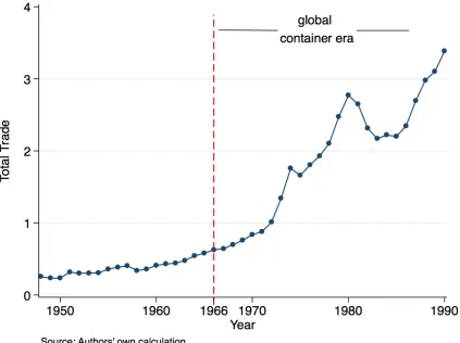
[image:2.595.93.516.287.603.2]One of the most striking developments in the global economy since World War II has been the tremendous growth in international trade. As shown in Figure 1, the increase in world trade accelerated dramatically during the early 1970s, with world trade growing in real terms from 0.45 trillion dollars in the early 1960s to 3.4 trillion dollars in 1990, by about a factor of 7. A central question is what accounts for this dramatic growth in world trade. Two broad explanations have been identified: (i) trade policy liberalization and (ii) technology-led declines in transportation costs.2
Figure 1: The growth of world trade (deflated): 1948-1990
A vast literature on transportation economics has argued that containerization was the major change in 20th century transportation technology responsible for the acceleration of the globalization of the world economy since the 1960s.3 Figure 1 reveals that the dramatic increase in the growth in world trade appear to have coincided with the genesis of the global container era which can be dated
2 See Krugman (1995) for a prominent discussion on the growth of world trade.
3See Levinsohn (2006) and Donovan and Booney (2006) for good overviews of containerization and references to case
to 1966. However, a quantitative assessment on the effect of containerization on international trade appears to be missing. In fact, in an influential and well-researched book on the history of the container revolution, Mark Levinson (2006, p.8) asserts that "how much the container matters to the world economy is impossible to quantify". Our paper challenges this claim and suggests an empirical identification strategy that allows us to estimate the effect of containerization on international trade.
Containerization was invented and first commercially implemented in the US in the mid 1950s. After ten years of US innovation in port and container ship technologies, followed by the international standardization in 1965, the adoption of containerization in international trade started in 1966. Numerous case studies have documented that containerization has not only affected the operation and relocation of ports but the entire transportation industry.4 Specifically, the introduction of containerization has gone hand in hand with the creation of the modern intermodal transport system, facilitating dramatic increases in shipping capacities and reductions in delivery times through intermodal cargo movements between ships, trains and trucks.
Based on information scattered in transportation industry journals, we are able to identify the year in which a country entered the container age by first processing cargo via port and railway container facilities. Since the intermodal feature of the container technology required a transformation of the entire journey from the factory gate to the customer, we capture containerization as a country-pair specific qualitative technology variable that switches from 0 to 1 when both countries entered the container age at time t. Time and cross-sectional variation of this technology variable permits us to apply it to a large panel of bilateral trade flows for 157 countries during the time period of 1962-1990. Our time horizon includes 4 years of pre-container shipping in international trade, the period of global container adoption 1966-1983 and 7 years where no new country in our sample started to adopt containerization. Since our time horizon precedes the period of dramatic reductions in the costs of air transport, our study excludes the other major 20th century change in the global transportation sector. Because our data provides information on both port and railway containerization, our analysis captures the main modes of international transport during this period.5
Our empirical strategy exploits cross-sectional and time variation in the economy-wide adoption of container facilities and product level variation in containerizability in a difference-in-difference framework. The inclusion of country-and-time effects allows us to capture multi-lateral
4 See McKinsey, (1967, 1972) and the various issues in Containerization International (1970-1992).
5 Since the adjustment of container transportation via truck followed the adoption of port and railway container facilities
resistance identified by the structural gravity literature and other time-varying factors that might be correlated with countries’ decisions to invest in container ports6. Difficult to measure geographic
factors, like government desires to act as container port hubs, are captured by country-pair specific fixed effects. The panel nature of our data set permits us not only to estimate the cumulate average treatment effects (ATE) of containerization but also allows us to evaluate the size of the estimates in comparison to the time-varying trade policy liberalization variables that have been used in the literature.
Although the introduction of containerization resulted in economy-wide changes of transportation infrastructure, the impacts are expected to be uneven among traded product groups. For this reason and because not all products are containerizable, we examine variations in bilateral trade flows at a disaggregated level. This allows us to exploit product level variations in containerizability and container usage amongst adopters of the container. We exploit a 1968 study by the German Engineers Society which classifies 4-digit product groups as to whether they were suitable for container shipments as of 1968 and use also more recent US Census product level data on container usage.
Restricting our sample to North-North trade, which are mainly the early adopters, our benchmark specification which uses differences in the timing of adoption between countries suggests that the cumulative average treatment effect (ATE) of containerization was about 1,240% after 15-years. For all countries we find an effect that is smaller but still of economic importance at 900%. Although the contemporaneous effect of containerization is quite similar to the North-North analysis, the dynamic effects of containerization are much weaker for trade flows that involve developing economies. This might be explained by the reduced penetration of the technology to include other parts of the transport system in developing countries.
Interpreting the results from the above regressions relies on trade between non-containerized pairs of countries providing a valid counterfactual. When testing this using information on trade flows in the pre-containerization period, we find that this is satisfied for North-North trade in the benchmark specification, but not consistently so across all of the robustness tests that we provide. For the sample containing all countries (early and later adopters), we consistently find pre-container differences in the growth rate of bilateral trade. Therefore, even though the literature suggests that the returns to containerization were much more uncertain for the early adopters (North-North trade), an identification strategy based solely on differences in the timing of adoption of the container does
6 See Feenstra (2004, p.161-163) for a good discussion on the use of country fixed effects to deal with multilateral
not appear capable of providing convincing evidence of causal effects. The additional trade can be attributed to the container revolution only with caution.
Those estimates may also be subject to endogeneity concerns; countries did not choose to adopt this new transportation technology randomly and our estimates may be upward biased. To address this we present a second set of estimates that exploits the containerizability of some products. From this we continue to provide evidence that containerization did affect bilateral trade flows, albeit more modestly compared to estimates based on differences in the timing of adoption. Comparing the change in bilateral trade of containerizable products versus non-containerizable products amongst pairs of countries that had adopted the container, we find significant differences in the growth of trade in the order of 17.4% for North-North trade and 14.1% for World trade, but where the latter occur 10-15 years after containerization. Comparing these to the estimates derived purely from differences in the timing of adoption indicates that container was more important as an explanation of differences in the growth of trade between countries across time, rather than across products. Pre-containerization differences in trade flows are however less apparent when using differences in trade flows in the product dimension, increasing the likelihood that these estimates are causal.
Our paper contributes to the broader literature that aims to quantify the effects of changes in transportation technology on economic activity. Starting with Fogel’s (1964) pioneering study on the effects of US railroads on economic growth, a number of studies have investigated the effects of railroad construction on economic performance and market integration. Based on detailed archival data from colonial India, Donaldson (2012) provides a comprehensive general equilibrium analysis of the impacts resulting from the expansion of India’s railroad network during 1853-1930.7 While the
introduction of rail and steamships were the main changes in transportation technology that underpinned the first wave of globalization (1840s-1914), students of transportation technology and prominent commentators link the post World War II growth of world trade to containerization. For example, Paul Krugman writes (2009, p. 7):
“The ability to ship things long distances fairly cheaply has been there since the steamship and the railroad. What was the big bottleneck was getting things on and off the ships. A large part of the costs of international trade was taking the cargo off the ship, sorting it out, and dealing with the pilferage that always took place along the way. So, the first big thing that changed was the introduction of the container. When we think about technology that changed the world, we think
7 Donaldson (2012) tests several hypotheses of the effects of railroads that he derives from a region,
about glamorous things like the internet. But if you try to figure out what happened to world trade, there is a really strong case to be made that it was the container, which could be hauled off a ship and put onto a truck or a train and moved on. It used to be the case that ports were places with thousands and thousands of longshoremen milling around loading and unloading ships. Now longshoremen are like something out of those science fiction movies in which people have disappeared and been replaced by machines”.
The current state of the empirical trade literature supports the view that the decline in transportation costs did not play a significant role in the growth of world trade. In an influential paper studying the growth of world trade, Baier and Bergstrand (2001) have found that the reduction in tariffs is more than three times as important as the decline in transportation costs in explaining the growth of OECD trade between 1958-60 and 1986-88.8 In his survey of how changes in transportation costs have affected international trade in the post world War II period, Hummels (2007) has detected an actual increase in ocean shipping rates during 1974-84, a period after the adoption of containerization in the US. Using commodity data on US trade flows, Hummels finds that freight cost reductions from increasing an exporter’s share of containerized trade have been eroded by the increase in fuel costs resulting from the 1970s hike in oil prices.9
Our identification strategy is rooted in our reading of the historical literature which suggests that containerization resulted in far reaching complementary technological and organizational changes in port and railway services that affected economies’ entire transportation sectors.10 In fact, our findings confirm Hummels’ (2007, p. 144) intuition that “the real gains from containerization might come from quality changes in transportation services…To the extent that these quality improvements do not show up in measured price indices, the indices understate the value of the technological change”. Our findings are also compatible with Yi (2003) who has stressed the role of vertical specialization and disintegration of production as a major factor in explaining the growth of world trade.11 Experts in transportation economics have emphasized repeatedly that the global
8 Because of data limitations, Baier and Bergstrand (2001, Table 1, p.14) use only a multi-lateral rather than a bilateral
index of changes in transportation costs. Their index suggests that Austria’s transportation costs versus the rest of the world have actually increased between 1958 and 1986, which does not appear plausible. Although land-locked, Austria has been an early entrant in the container age through their construction of container railway terminals in 1968 which connected it to the main container ports in Europe.
9 Another study that investigates the effects of containerization on US imports in the post adoption period is Blonigen and
Wilson (2008). Building on Clark, Dollar and Micco (2004), they estimate the effects of port efficiency measures on bilateral trade flows and find that increasing the share of trade that is containerized by 1 percent lowers shipping costs by only 0.05 percent.
10 A study by Eyre (1964) claims that during the pre-container age ocean shipping costs accounted only for 25% of the
total door-to-door costs of shipping a truckload of medicine from Chicago to Nancy in France.
11 Baier and Bergstrand (2001) are quite honest in pointing out that their final goods framework excludes this potential
diffusion of intermodal transport was a prerequisite for the disintegration of production and the establishment of global supply chains (Notteboom and Rodrigue, 2008).
The next section of the paper provides a historical discussion on the origins and effects of containerization. Our historical narrative fulfills two purposes. First, by describing the different channels through which container adoption reduced trade costs we point to the mechanisms that appear to be responsible for our estimated effects. Second, our historical evidence on the speed of diffusion of container technology within the transportation structure of two selected economies provides the rationale for our identification strategy of capturing containerization. Section three introduces our empirical specifications and discusses our empirical findings. Section four concludes.
2. The container revolution and intermodal transport
“Born of the need to reduce labor, time and handling, containerization links the manufacturer or producer with the ultimate consumer or customer. By eliminating as many as 12 separate handlings, containers minimize cargo loss or damage; speed delivery; reduce overall expenditure”.
(Containerisation International, 1970, p. 19)
2.1 Historical background
Before the advent of containerization, the technology for unloading general cargo through the process of break-bulk shipping had hardly changed since the Phoenicians traded along the coast of the Mediterranean. The loading and unloading of individual items in barrels, sacks and wooden crates from land transport to ship and back again on arrival was slow and labor-intensive. Technological advances through the use of ropes for bundling timber and pallets for stacking and transporting bags or sacks yielded some efficiency gains, but the handling of cargo was almost as labor intensive after World War II as it was during the beginning of the Victorian age. From a shipper's perspective, often two-thirds of a ship's productive time was spent in port causing port congestion and low levels of ship utilization. Following the spread of the railways, it became apparent already during the first era of globalization that the bottleneck in freight transport was at the interface between the land and sea transport modes.
The genesis of the container revolution goes back to April 26, 1956 when the Ideal- X, made its maiden voyage from Port Newark to Houston, Texas. The ideal X was a converted World War II tanker that was redesigned with a reinforced deck to sustain the load of 58 containers. As so common in the history of innovation, the breakthrough of containerized shipping came from someone outside the industry, Malcom McLean, a trucking entrepreneur from North Carolina. Concerned about increased US highway congestion in the 1950s when US coastwise shipping was widely seen as an unprofitable business, McLean's central idea was to integrate coastwise shipping with his trucking business in an era where trucking and shipping were segmented industries. His vision was the creation of an integrated transportation system that moved cargo door to door directly from the producer to the customer. The immediate success of the first US container journey resulted from the large cost savings from the mechanized loading and unloading of containerized cargos. Shortly after the Ideal-X docked at the Port of Houston, McLean's enterprise, which later became known as Sea-Land Service, was already taking orders to ship containerized cargo back to Newark.
The 1956 container operation by the Ideal X involved a ship and cranes that were designed for other purposes. McLean's fundamental insight, which was years ahead of his time, was that the success of the container did not rest simply on the idea of putting cargo into a metal box. Instead, it required complementary changes in cranes, ships, ports, trucks, trains and storage facilities. Three years following Ideal X's maiden voyage, container shipping saw additional savings through the building of purpose-built container cranes followed by the building of large purpose-built containerships. On January 9, 1959 the world's first purpose-built container crane started to operate and was capable of loading one 40,000-pound box every three minutes. The productivity gains from using this container crane were staggering, as it could handle 400 tons per hours, more than 40 times the average productivity of a longshore gang.12 Investment in larger shipping capacity became now
profitable since containerization dramatically reduced a ship's average time in ports.
Given the large investment costs, industry experts revealed a considerable amount of uncertainty and skepticism regarding the success of the container technology at the time. Many transportation analysts judged container shipping as a niche technology and did not anticipate the dramatic transformations that this technology was about to bring to the entire domestic and international transportation sector. In the first decade following the Ideal- X’s maiden voyage, innovation and investment in container technology remained an American affair. But, as Levinson (2006, p. 201) points out, "ports, railroads, governments, and trade unions around the world spent those years studying the ways that containerization had shaken freight transportation in the United
States". The early initiatives came from US shipping lines and by the early 1960s, containerization was firmly established on routes between the US mainland and Puerto Rico, Hawaii and Alaska. Ten years of US advancement in container technology set the foundation for containerization to go global in 1966.13 In that year, the first container services were established in the transatlantic trade between the US and European ports in the UK, Netherlands and West Germany.
2.2 Economic effects of containerization
From a transportation technology perspective, containerization resulted in the introduction of intermodal freight transport, since the shipment of a container can use multiple modes of transportation -ship, rail or truck- without any handling of the freight when changing modes. By eliminating sometimes as many as a dozen separate handlings of the cargo, the container resulted in linking the producer directly to the customer. Since containerization resulted in a reduction of the total resource costs of shipping a good from the (inland) manufacturer to the (inland) customer, its impact is not adequately captured by looking at changes in port-to-port freight costs.14
Containerization started as a private endeavor by the shipping lines. In the early stages, shipping lines had to bear most of the costs since many ports such as New York and London were reluctant to spend significant funds on ‘a new technology’ with uncertain returns at the time. Many shipping lines had to operate from small and formerly unknown ports and install their own cranes. The process was extremely expensive. After the container proved to be successful, ports warmed up to containerization and a race started among ports to attract the most shipping lines by building new terminals and providing the infrastructure to handle containers. Containerization required major technological changes in port facilities, which often led to the creation of new container ports. In the United States, the new container ports in Newark and Oakland took business from traditional ports like New York and San Francisco. In the UK, the ports of London and Liverpool, which handled most of the British trade for centuries, lost their dominant position to the emerging container ports of Tilbury and Felixstowe.
In many countries, port authorities fall under the administration of the government. Because of the high costs, careful planning and analysis had to be undertaken by governments to study the
13 Australia was the first country to follow the US and adopted container technology in 1964, but not in international
trade.
14 Reliable data on comparable changes in door-to-door and ocean freight rates before and after containerization are not
available. However, Eyre (1964) uses data from the American Association of Port Authorities to illustrate the
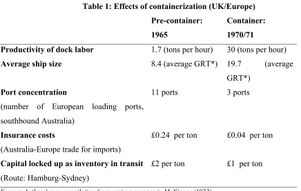
feasibility of containerization. In the UK, the government commissioned McKinsey (1967) to conduct a cost and benefit analysis before spending significant public funds on container port facilities. Five years later, McKinsey (1972) provided a quantitative assessment of the effects of containerization following the first five years after its adoption in the UK and Western Europe. Table 1 provides a summary of the sources and magnitude of resource savings from the adoption of container technology between 1965 and 1970/71.
Table 1: Effects of containerization (UK/Europe) Pre-container:
1965
Container: 1970/71
Productivity of dock labor 1.7 (tons per hour) 30 (tons per hour)
Average ship size 8.4 (average GRT*) 19.7 (average
GRT*) Port concentration
(number of European loading ports, southbound Australia)
11 ports 3 ports
Insurance costs
(Australia-Europe trade for imports)
£0.24 per ton £0.04 per ton
Capital locked up as inventory in transit (Route: Hamburg-Sydney)
£2 per ton £1 per ton
Source: Authors' own compilation from various sources in McKinsey (1972). *GRT is gross registered tonnage which is a ship's total internal volume expressed.
One of the major benefits of containerization was to remove the bottleneck in freight transport in the crucial land-sea interface. The construction of purpose-designed container terminals increased the productivity of dock labor from 1.7 to 30 tons per hour (Table 1). Improvement in the efficiency and speed of cargo handling allowed shipping companies to take advantage of economies of scale by more than doubling the average ship size. The resulting increase in port capacity provided opportunities and pressures for the inland distribution of maritime containers. In the UK the introduction of railway container terminals went in tandem with port containerization and by 1972 the Far East service alone already operated trains between an ocean terminal and six inland rail terminals.
eliminated the notion of a port hinterland and containerized freight became concentrated in a few major terminals. For example, whereas in 1965 ships in the (southbound) Australian trade called at any of 11 loading ports in Europe, by 1972 the entire trade was shared among the three ports of Hamburg, Rotterdam and Tilbury. Within a few years, a hub-and-spoke system already emerged.
A major benefit of sealing cargo at the location of production in a box to be opened at the final destination is that it reduced the pilferage, damage and theft that were so common in the age of break-bulk shipping. A common joke at the New York piers was that the dockers’ wages were “twenty dollars a day and all the Scotch you could carry home”. The resulting reduction in insurance costs from containerization was considerable. On the Australia-Europe trade, between 1965 and 1970/71 the insurance costs fell from an average of 24 pennies per ton to 4 pennies per ton (Table 1).
Intermodal transport also decreased the time in transit between cargo closing and availability. Containerization cut the journey between Europe and Australia from 70 to 34 days. Given that the average cargo at the time was worth about £60 per ton and assuming that the opportunity cost of capital tied up in transit is about 15%, the 36-day improvement cut the capital cost of inventory by about a half (Table 1).
The importance of labor in the operation of ports in the pre-containerization age resulted in the emergence of strong labor unions, which resisted not only labor-saving organizational changes but were also well-organized and effective in calling for strikes. The replacement of capital for labor, which emerged through containerization, ended the frequent delays and uncertainties in shipping caused by these strikes.15
2.3 Diffusion of container technology
The early use of containers was driven by private shipping companies who used container sizes and loading devices that best fit their cargo and shipment routes. The first fully containerized ships used 35-foot containers, which was the maximum allowable length for truck traffic on US highways. However, since a fully loaded container of this size was too heavy for a crane to lift, other companies used much smaller sizes which could be much easier stacked and moved with forklifts. A major force for the international adoption and diffusion of container technology was the standardization of container sizes. The standardization process was initiated in the US by the Federal Maritime Board and involved stakeholders from the maritime sector, truck lines, railroads and trailer manufacturers. In 1961, the Federal Maritime Board established the standard nominal dimension of containers - 8 feet wide, 8 feet high and 10, 20, 30 and 40 feet long- and announced that only
15 We thank David Smith, Economics Editor of the Sunday Times, for pointing out the elimination of strikes as a channel
containerships designed for these sizes were able to receive construction subsidies from the US government.
Following the setting of standards in the US, the International Standards Organization (ISO) started to study containerization with the purpose of establishing worldwide guidelines as a prerequisite for firms and governments investing in internationally compatible container technology. Following a compromise between US and European interest groups, the ISO formally adopted the 10- ,20- , 30- and 40-foot containers plus a few smaller sizes favored by the Europeans as ISO standards in 1964. Besides container size, strength requirements and lifting standards were other major aspects the ISO was able to standardize in 1965. The standardization of container technology was followed by the rise of container leasing companies who had now the incentives to expand their fleets and allowing shippers the flexibility to lease containers and therefore significantly reducing the fixed costs of using this technology. The ability for land and sea carriers to handle each other’s containers in different locations set the foundation of global container adoption around the globe.
The adoption of container technology in international trade started in 1966 and the period of 1966-1983 has been labeled by geographers as the era of global diffusion of container technology around the globe (Kuby and Reid, 1992).16 The introduction of container technology started with a
country’s investment in container port facilities but quickly progressed to engulf other parts of the transportation network, like rail and road transport. Accompanying technological changes were larger ships and trains and increased use of computers and telecommunications for managing and tracking intermodal movement.
From our calculations of an underlying sample of 157 countries, 122 entered the container age by first processing container cargo via port or railway facilities between 1966 and 1983 while 35 countries remained uncontainerized as of 1990. Appendix Table 3 lists all sample countries and reveals considerable cross-sectional and time variation of countries’ adoption of container port facilities during the sample period.
Historical accounts suggest an important role for the US military build-up in Vietnam to stimulate the diffusion of container technology in East Asia. Initially, US military leaders were skeptical about the adoption of container technology for the shipment of military cargo. However Malcom McLean’s persistence and vision that his brainchild could alleviate the logistical challenges associated with the rapid buildup of military forces in Vietnam after 1965 won the argument in favor of the container. And by 1970 half of the military cargo was already containerized on critical
16 According to Kuby and Reid (1992, p.285) “…after 1982 the industry reached maturity, characterized by low margins
routes.17 A key feature of the military use of containerization during the Vietnam conflict was that McLean’s ships were loaded with military freight on their west-bound journey to Vietnam while the return east-bound journey carried initially empty containers. Levinson (2006) has argued that the availability of this container capacity played a role in the diffusion of containerization.18
2.4 Capturing the degree of container utilization for two island economies
How quickly did containerization diffuse through an economy’s transportation sector following its initial adoption of container port facilities? First, some tradable goods like assembled automobiles, heavy machinery, construction equipment and some steel products can’t be put into containers. Second, technological advancement in container technology has expanded the range of containerizable products over time. For example, initially food products were not containerizable, but through the development of refrigerated containers, food became containerizable in later years. A measure of the degree of an economy’s container utilization in its international trade is the ratio of the economy’s traded containerized cargo dived by its total trade of containerizable cargo. The container utilization index for an economy i at time t, ContUtilit, is then given by:
ContUtilit = (containerized cargoit)/(containerizable cargoit) (1)
Fortunately, the denominator of (1) can be calculated based on a study by the Verband deutscher Ingenieure (German Engineers Society) which classified 4-digit SITC industries according to whether they were suitable for containers as of 1968.19 The calculation of (1) faces the challenge that containers can cross borders through different modes of transport (sea, rail, truck and air) and that there exist no data on traded container tonnage via rail, trucks or air. However, for island economies like the UK and Japan, where (at the time) the majority of international trade went through sea ports, it is possible to trace their growth of container utilization following their first adoption of the technology.20 For these two countries, (1) can be calculated by combining data on container tonnage going through seaports available from Containerisation International with tonnage
17 Levinson (2006), p. 183.
18 While working on this project, we became aware of the very interesting work by Gisela Rua (2014) who formally
investigates the determinants of the diffusion of containerization. She finds that the decision of later adopters is influenced by their trade with the US. Her study is based on detailed data on port container usage, but does not focus on containerizable versus non-containerizable products.
19 The engineering study classifies industries into Class A: suitable for containers, Class B: goods of limited suitability
for containers and Class C: goods not suitable for containers as of 1968. For the purpose of constructing our container utilization index, we only include goods in Class A as containerizable. These are listed in Appendix Table 4.
of trade in containerizable industries provided by the OECD International Trade by Commodity Statistics.
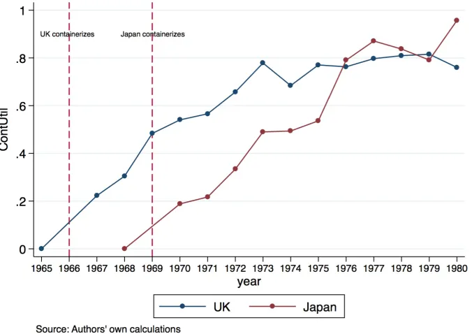
[image:14.595.133.471.335.574.2]Figure 2 depicts the time change in the container utilization index (1) for the UK and Japan during the period of 1965-1980.21 The UK adopted its first container facilities in 1966 and the technology diffused quite rapidly. The utilization grows from 20% in 1967 to about 80% in 1973 and remains then quite flat, which can be explained by the oil shock and the recession following the oil crisis. The picture for Japan is quite similar. Japan adopted containerization in 1969 and the utilization index grows from 20% in 1970 to about 50% in 1973 and then to over 80% during the late 1970s.22
Figure 2: Changes in container utilization in the UK and Japan
2.5 Containerization and land transport
A defining element of the adoption of container technology is the creation of intermodal transport. Containerization was quickly picked up by railways in different countries. For example, in response to port containerization, and in an effort to avoid being left out, the railways of Europe
21 Total trade is defined as (exports+imports)/2. Because of missing data in the years of container adoption, the graph
depicts linear segments between 1965 and 1967 for the UK and between 1968 and 1970 for Japan.
22 Rua’s (2014, p.36) documentation of a relatively lower container usage in her broad sample of countries in her Figure 1
came together in 1967 and formed Intercontainer, The International Association for Transcontainer Traffic. This company was formed to handle containers on the Continent and compete with traditional shipping lines.23 Railway containerization allowed landlocked countries like Austria and
Switzerland to ship their goods in containers to seaports in neighboring countries destined to overseas destinations. In many cases, this was cheaper and less laborious than road transportation. In a comprehensive cost study for the UK, McKinsey (1967) calculated that container transport was cheaper by rail than truck for journeys above 100 miles. Containerisation International (1972) estimated that the cost of moving 1 TEU (twenty foot equivalent unit container) between Paris and Cologne in 1972 was about 75% of the equivalent road costs.24
Although the majority of non-land locked countries adopted railway container facility after their introduction of container seaports, for some the ordering was reversed. For example, Norway entered the container age via their railway network in 1969, five years before the adoption at their seaports. This suggests that countries could enter the container age either through the introduction of rail or sea ports container facilities.25
3. Empirical implementation
3.1 Quantifying containerization
Our objective is to estimate the effect of containerization on international trade. The key question that arises is how to capture this technological change quantitatively. Since the adoption of container technology triggered complementary technological and organizational changes that affected an economy’s entire transportation system this suggests quantifying this technological change at the economy level. If economy level data on the international shipments via rail or truck were available, the container utilization index (1) would be a sensible measure of the technological change. However, because of the absence of the appropriate data and the occurrence of technological change regarding containerizability, we can’t go this path. Alternatively, the quick rise in the container utilization for the UK and Japan justifies quantifying containerization by a
23 At the time, British Rail was already operating a cellular ship service between Harwich, Zeebrugge and Rotterdam and
a freightliner service between London and Paris. Initially 11 European countries formed Intercontainer and were later joined by 8 more.
24 We are not aware of any studies that document the spread of road containerization equivalent to that for port or rail
containerization. The historical narrative suggests however that the developed countries that we focus on this was concurrent to port and/or rail containerization. Outside of this the assumption is less certain. We found for example photographic evidence that the Comoros Islands were using containers without either rail or port container depots (they were instead dropped onto modified rowing boats).
25 Besides containerization, advances in information technologies and logistics, in particular ‘just in time’ manufacturing
qualitatively variable that switches from 0 to 1 when country i entered the container age at time t. We define entrance into the container age as the first recorded use of either seaports or inland railway ports. An advantage of this specification is that it captures the intermodal aspect of containerization since it encompasses land-locked countries like Austria and Switzerland who entered the container age via rail connection to the container seaports of Rotterdam and Hamburg. Based on the recorded information provided in the published volumes of Containerisation International between 1970 and 1992, we construct a time-varying container adoption variable for country i, adoptcontit, defined as: 𝑎𝑑𝑜𝑝𝑡𝑐𝑜𝑛𝑡!" = 10 𝑖𝑓 𝑜𝑡ℎ𝑐𝑜𝑢𝑛𝑡𝑟𝑦𝑒𝑟𝑤𝑖𝑠𝑒 𝑖 𝑢𝑠𝑒𝑠 𝑠𝑒𝑎 𝑜𝑟 𝑟𝑎𝑖𝑙 𝑐𝑜𝑛𝑡𝑎𝑖𝑛𝑒𝑟 𝑝𝑜𝑟𝑡𝑠 𝑖𝑛 𝑦𝑒𝑎𝑟 𝑡 (2)
Although a country’s adoption of container technology is expected to have some effect on its overall trade, the nature of container technology suggests that containerization is more adequately captured in a bilateral trading context since this allows us to specify the presence of container technology of a country’s trading partner. This suggests capturing containerization by a time-varying bilateral technology variable, defined as:
𝑐𝑜𝑛𝑡!"# = 1 𝑖𝑓 𝑖 𝑎𝑛𝑑 𝑗 ℎ𝑎𝑣𝑒 𝑏𝑜𝑡ℎ 𝑐𝑜𝑛𝑡𝑎𝑖𝑛𝑒𝑟𝑖𝑧𝑒𝑑 𝑝𝑜𝑟𝑡𝑠 𝑜𝑟 𝑟𝑎𝑖𝑙𝑤𝑎𝑦𝑠 𝑖𝑛 𝑦𝑒𝑎𝑟 𝑡
0 𝑜𝑡ℎ𝑒𝑟𝑤𝑖𝑠𝑒 (3)
From an econometric point of view, there are several advantages quantifying containerization by a time-varying bilateral variable, most notably the ability to include various types of fixed effects. Since we are interested in exploring causal effects of container technology on trade, one worries about potential selection bias in the adoption of container technology. Armed with “ex post” knowledge that containerization revolutionized global freight transport, one would be inclined to infer that countries that initially traded a lot would be most likely to adopt container technology. However, as we have pointed out in our historical narrative in section 2, from the relevant decision point of view of the 1960s, containerization was by many viewed as a niche technology with little perceived impact on the volume of international trade. For example, Levinson (2006, p. 276) writes:
almost everything long distances simply did not occur to him. Chinitz was hardly alone in failing to recognize the extent to which lower shipping costs would stimulate trade. Through the 1960s, study after study projected the growth of containerization by assuming that existing export and import trends would continue, with the cargo gradually shifted into containers”.
The second component of our identification strategy exploits the fact that not all products are containerizable. Specifically, we take advantage of the 1968 study by the German Engineer’s society, reported in Containerisation International Yearbook (1971), which classifies 4-digit product lines whether they are suitable for container shipments as of 1968.26 Unfortunately, we are not aware of any other study that provides a classification of product containerizability after 1968.27 However, the Foreign Trade Statistics Division of the US Census Bureau collects port level data on the mode of transportation of US imports and exports by products which goes back to 2003.28 Because the US Census data provides information on whether imports entered the US via container vessels, it allows us to provide adjustments on products that were categorized as containerizable or uncontainerizable in 1968.
Based on these two data sources we construct three measures of containerizability. We use the 1968 classification within our benchmark regressions, based on the arguments that this measure is based on generic engineering criteria, while the US Census Bureau data capture revealed containerizability; and that the date of this classification, 1968, is closer to the major adoption period, which ran between 1966 and 1983. Results for the second and third measures can be found in the robustness section and are constructed using the US Census Bureau data to either redefine the ‘non-containerizable control group’ or both the treatment and the control group. The second measure uses the US Census data to reduce the 1968 control group of ‘non-containerizables’ by excluding products within this category with relatively high container usage in 2003.29 The third measure makes the
same adjustment to ‘non-containerizable’ products and in addition excludes from the category of ‘containerizable’ products those with low container usage in 2003.30 Containerizability of product group k is captured by the categorical variable prodk, defined as:
𝑝𝑟𝑜𝑑!= 1 𝑖𝑓 𝑘 𝑖𝑠 𝑐𝑙𝑎𝑠𝑠𝑖𝑓𝑖𝑒𝑑 𝑎𝑠 𝑐𝑜𝑛𝑡𝑎𝑖𝑛𝑒𝑟𝑖𝑧𝑎𝑏𝑙𝑒0 𝑖𝑓 𝑘 𝑖𝑠 𝑛𝑜𝑡 𝑐𝑜𝑛𝑡𝑎𝑖𝑛𝑒𝑟𝑖𝑧𝑎𝑏𝑙𝑒 𝑖𝑛 1968 𝑤𝑖𝑡ℎ𝑜𝑢𝑡/𝑤𝑖𝑡ℎ 2003 𝑎𝑑𝑗𝑢𝑠𝑡𝑚𝑒𝑛𝑡 𝑖𝑛 1968 𝑤𝑖𝑡ℎ𝑜𝑢𝑡/𝑤𝑖𝑡ℎ 2003 𝑎𝑑𝑗𝑢𝑠𝑡𝑚𝑒𝑛𝑡 (4)
26 Recall that we used this classification in the construction of our utilization index (1) in Figure 2.
27 For example, technological progress expanded the scope of products that become containerizable, such as automobiles. 28 The data is accessible via USA trade online, categorized as Port Data (6-digit, HS level).
29 In the adjustment we ranked products according to the container usage ratio, (containerized trade in k)/(total trade in k).
We then dropped those products from the control group for which the container usage ratio was larger than in the bottom quartile of the distribution. We chose 2003 because this is the earliest year for which this data is available.
30 We identify such products by calculating the share of US trade carried by container in 2003 and excluding from the
3.2 Research design and empirical specification
The time frame of our analysis is dictated by the availability of bilateral trade data at the product level and the timeline of container adoption in international trade. Fortunately, the world trade data set compiled by Feenstra et al. (2005) goes back to 1962 and covers bilateral trade flows from 1962-2000 at the 4-digit product level.31 Since the adoption of containerization in international trade started in 1966 and ended in 1983, we chose 1962-1990 as our sample period, which includes 4 years prior to the first adoption and 7 years past the last adoption year. We chose to exclude the 1990s because of both the redrawing of the political map after the end of the Cold War and the reduction in the costs of air transport which started to kick in in the early 1990s. Although there is limited data on changes in the mode of transport in international trade, a reading of the transportation industry literature suggests that during our chosen sample period containerization was the main technological change affecting the three major modes of transport (sea, rail and road) in international trade.
Our outcome variable pertains to the bilateral trade flows between countries i and country j in product group k at time t, 𝑥!"#$. Our empirical equation to be estimated is given by32:
∆ln𝑥!"#$ =𝛽!+𝛽!∆𝑐𝑜𝑛𝑡!"#+𝛽!∆𝑐𝑜𝑛𝑡!"#∙𝑝𝑟𝑜𝑑!+𝛽!∆𝑃𝑜𝑙𝚤𝑐𝑦!"#+ 𝛽!𝐷!"#$+ 𝑢!"#$. (5)
Our key explanatory variables are the time varying bilateral container variable contijtfrom (3) and the
interaction of this variable with the product containerizability variable prodk from (4). 𝑃𝑜𝑙𝚤𝑐𝑦!"#
denotes a vector of time-varying bilateral policy variables, 𝐷!"#$ includes a (large) vector of country- time and product-time specific fixed effects and 𝑢!"#$ denotes the error term.
We opted for first differencing the data across our 5-year time periods such that our dependent variable becomes Δxijkt=xijkt-xijk(t-1).33 Wooldridge (2002, chapter 10) suggests that
first-differencing a panel data set yields advantages if unobserved heterogeneity in trade flows is correlated over time. So we regress Δxijkt on Δcontijktand the other first differenced country-pair
time-variant policy variables like being in a regional trade agreement (rta) or a member in the GATT. The time varying bilateral container variable Δcontijt captures the effect on the change in the
log of bilateral-product trade flows from differences in the timing of adoption of the container
31 The data set is constructed from the United Nations trade data and is available from NBER. 32 For efficiency of exposition, we omitted all lags of the explanatory variables.
between bilateral pairs.34 The interaction of this with the containerizability variable allows for differences in these effects for products that were suitable to be placed inside containers versus those that were not. This difference compared to non-containerizable products might include reductions in the time spent at port due to greater inter-modality of the logistics chain, reduced pilfering of goods, reduced insurance costs etc. When using this measure of containerization the effects of containerizability are measured relative to trade in non-containerizable products amongst country-pairs that had adopted the container. In both cases, the anecdotal evidence suggests that containerization led to the increased growth of trade and we therefore anticipate the coefficient on these variables to be positive. The countrywide changes in transport infrastructure which occurred in many countries when adopting the container would suggest there may be benefits for trade in all types of products and therefore the estimate of β1 will be larger than β2.
Interpreting the coefficients on the various container measures as capturing causal effects rests on the absence of omitted variables that are correlated with containerization and the error term from the regression. Concern for the effects of such variables motivates the inclusion of various fixed effects which we lay out below. It is possible that the effects of omitted variable bias remain however; the presence of time-varying bilateral shocks may have led to increased bilateral trade (faster growth), bringing forward in time the adoption of the container. We would over-estimate the effects of the container on bilateral trade in such a case. The presence of such shocks represents the main advantage to the inclusion of the containerizability interaction within equation (5). For the containerizability interaction to be interpreted as capturing causal effects requires that these unobservable shocks which determined the timing of adoption were not specific to containerizable products. While it is not possible for us to rule out this possibility, it is much more challenging to think what the omitted variables that affect trade in a sub-set of products that fitted inside containers might be. An interpretation of causal effects may therefore be considered more convincing in such a case.
An attractive feature of our panel specification is that it allows us to examine the dynamic aspects of containerization over a time period 1962-1990 characterized, as argued above, by little other transportation technological changes affecting international trade. Following the advice of the panel literature (Wooldridge, 2002) we examine changes in trade flows at 5-year intervals. In our context, the advantage of focusing on 5-year variations is that it mitigates the effect of differences in the speed of adoption (recall Figure 2) as well as allowing time for the build-up of the intermodal
34 We also use this change in logs to calculate the growth in trade that occurred as a result of the container (equal to
transport system. We estimate equation (5) on 7 time periods: 1962, 1967, 1972, 1977, 1982, 1987 and 1990.
To our knowledge, (5) is the first specification in the literature that identifies a time-varying bilateral technological change and aims to estimate its impact on international trade. An advantage of this specification is that allows for a comparison to other time-varying bilateral policy changes for a country pair i and j, like entrance into a regional trade agreement (rta) or both being a member in the GATT, which have been treated extensively in the literature. Specifically, (5) allows for a comparison between the estimate size of our container technology variable contijt and these trade
liberalization variables.35
An advantage of our panel specification is that it allows us to use fixed effects to avoid omitted variable biases associated with multi-lateral resistance terms identified from the structural approach to gravity.36 Specifically, the inclusion of time-varying importer (it), exporter (jt) and product (kt) fixed effects in 𝐷!"#$ capture time-varying product and country-specific factors that are either difficult to pin down or measure.37 In addition to multilateral resistance, the country-time dummies will also capture other changes that effect the growth of trade flows of a country. These include the infrastructure investments or other changes that were necessary to adopt the container and would otherwise be captured by the adoptcontit variable set out in equation (2). The ijk fixed
effects that are removed when we first difference the estimating equation allow for differences in the level of trade between country-pairs for each product k. To capture differences in the growth rate between country-pairs, in Table 3 below, where we consider a number of robustness issues of our main empirical findings, we add ij effects to the estimating equation.
3.3 Empirical findings
Although our entire data set covers a total of 157 countries, we initially report results for a sub-set of 22 industrialized countries, which we denote as North-North trade, in Table 2.38 Because
we expect a quicker and deeper penetration of container technology in industrialized countries (recall Figure 2), we initially apply equation (5) on an empirical domain where our technology variables are expected to capture relatively similar transformations of the transportation sector. In addition,
35 As we will discuss in 3.3, we also considered an interaction term between the container variable and the regional trade
agreement variable.
36 See Bergstrand and Egger (2011) and Feenstra (2004, chapter 5) for good surveys of the gravity literature.
37 Since the country-time fixed effects preclude the inclusion of time varying ‘economic mass’ variables like GDP and
GDP per capita, we refrain from calling our specification a gravity equation.
38 Our selection criterion was OECD membership as of 1990. It is probably of no coincidence that these countries were
restricting ourselves to North-North trade yields a full panel of country pairs. Afterwards, we extend the empirical domain to the total sample of 157 countries, labeled as ‘World Trade’ (columns 3 and 4).
Our dependent variable is the change in the log of exports and imports between a country pair
i and j in a 4-digit product line k. We only considered observations with trade occurring in at least one direction. The rationale behind this is that bilateral containerization should affect total bilateral trade rather than a specific direction. Because not all country pairs trade the same set of products in all years even in North-North trade, for which the panel is balanced on the ‘country-pair dimension’, the panel is ’naturally’ imbalanced in the product dimension. However, we restricted our sample by including only products which appear during the whole time period for at least one country pair.
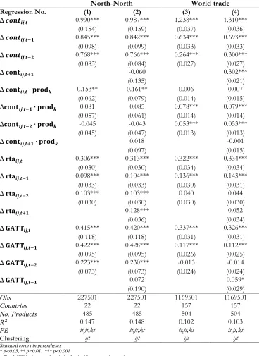
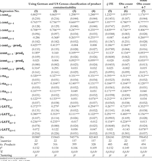
Our complete set of panel estimates of equation (5), including the lagged variables, is reported in columns (1) through (4) in Table 2. Depending on the specification, the number of products in our regressions varies between 485 and 504 with the corresponding total number of observations (or bilateral trade flows) varying between 227,501 (in regressions 1 and 2) and 1,169,501 (in regressions 3 and 4). All reported regressions include time-varying country fixed effects for each origin country, it, each destination country, jt, and time-varying fixed effects for each product, kt. Because our explanatory variables are more aggregated than our dependent variable, we also cluster by country-pair-year ijt. Our key explanatory variables are the contemporaneous and lagged effect of our binary container variable, Δcontij,t, and the contemporaneous and lagged effect of
this variable interacted with the product containerization variable, Δcontijt·prodk. Overall, the results
in Table 2 suggest that containerization is associated with statistically significant and economically large changes to the growth of bilateral trade irrespective of whether we base our measure of containerization on the timing of adoption or containerizability and irrespective of whether we restrict the analysis to North-North or World-Trade. The coefficients of the lagged effects of Δcontij,t
reveal that containerization had strong and persistent effects in some cases even 15 years after its bilateral adoption.
A key objective of our paper is to examine the causal effects of containerization on international trade using non-containerized bilateral pairs as a counterfactual. One requirement for such an interpretation is for the growth rate of trade to have been statistically similar for container and non-containerized pairs before the adoption of the container took place. Following the advice of Wooldridge (2002, p. 285), we add a future change of containerization, denoted by Δcontij,t+1, in our
regression equation (5). The size and statistical significance of Δcontij,t+1 can be viewed as a
the adoption of containerization. If the effect captured by the container dummy were simply related to growth trends already present in trade between that country-pair, we would expect the coefficient on years prior to the adoption of the container to be as large and significant as the coefficient on our variable of interest. Regression (2) in Table 2 also includes a pre-treatment variable on containerization and the other bilateral covariates rta and GATT for North-North trade and regression (4) performs the same exercise for the entire sample.
Regression (2) reveals that the coefficients of Δcontij,t+1 is statistically insignificant and also
very small compared to the contemporaneous and lagged variables, suggesting that the growth of trade between non-containerized countries was statistically similar to that for containerized countries prior to their containerization. Because the parallel trends assumption appears to be satisfied, the estimates can be interpreted as capturing a causal effect of containerization on North-North trade, if there are no other confounding factors that explain the decision to adopt the container and the growth in trade for adopting-pairs. We note that this result is not robust to the extensions we describe in the next section of the paper (Table 3). Hence, a causal interpretation is conditional on the specification.
Pre-adoption differences in trade flows are present in Table 2 when we extend the sample to cover World Trade. In column (4) the coefficients on Δcontij,t+1 are statistically significant and also
relatively large. This implies that if one includes less developed economies (or late adopters), the container coefficients are only suggestive of a high correlation as containerization was also adopted in response to increased growth in trade. Overall, these results are consistent with the historical narrative.
A somewhat different conclusion is reached for the containerizability interaction. The coefficient on Δcontijt+1·prodk is statistically insignificant, indicating no pre-adoption difference in
the growth rate of trade between products that were containerizable compared to the counterfactual of non-containerizable products. As a reminder this definition of containerizability uses the original 1968 German Engineers classification. This occurs for North-North trade in regression (2) and World trade in regression (4). To conclude from these tables as a whole, an identification strategy that exploits the product dimension of containerization appears a more promising route to capturing causal relationships.
containerization is capable of explaining a large part of the differences in growth rates of trade over time.
The coefficients on the lag variables reveal that over the next 5-year periods the effect of containerization was 0.842 and 0.766 log-points respectively. The contemporaneous and lagged effects of containerization sum to 2.595 (natural) log points, which equates to an annual growth rate of trade of 17.3% for a 15-year period. Using the mean (median) value for product-bilateral trade flows in our dataset of $2.5 million ($0.078 million) and our estimate of the cumulative ATE of 1,240% (=e2.595-1), this would imply that trade flows increased to $33.5 million ($1 million) because of containerization after 15-years.
The estimated coefficient on the interaction variables cont·prod in column (2) is noticeably smaller than for those based on the adoption of the container. From the discussion in Section 2.2 this was not unexpected and indicates that many of the changes that occurred during adoption of the container were not specific to containerizable products. This regression provides the smallest estimate of the trade effect derived from the introduction of the container within the paper. In column (2) the concurrent effect of containerization was to increase bilateral trade by 0.161 log-points for containerizable products relative to non-containerizable products (equivalent to an annual growth rate of 3.2% for 5-years, or a cumulative ATE of 17.4%). The lagged interaction effects are not statistically significant, indicating that the growth rates of trade flows in containerizable and non-containerizable products were statistically similar beyond this 5-year period. This result suggests that containerization gave a permanent boost to the level of bilateral trade in containerizable products through a short-lived increase to the growth rate of trade.
How do the effects of containerization compare to the time-varying trade policy variables that are also included in the regression? As mentioned above, we included two sets of policy variables. The rta dummy indicates whether a country pair ij belonged either to the same regional free trade block or had a free trade agreement in a specific year. The GATT variable switches to 1 if both countries i and j are members of the GATT, the precursor of the WTO, at time t. The inclusion of lagged effects permits us also to investigate the dynamic effects of these variables.
Overall, we find that the estimated effects of containerization are generally much bigger than the estimated effects of the trade policy variables in all specifications. This occurs even if we allow for interaction effects between the container technology and the various trade policy variables, the coefficients for which are insignificantly different from zero.39 The concurrent and the first two lags of the rta variable have the expected positive sign and are highly significant. The concurrent effect of
39 For this reason we choose not to report the results from this regression. The results are available from the authors on
a free trade agreement is to raise trade by an average of 0.313 log points (an increase to the annual growth rate of 6.2%), which is about a third of the concurrent effect of containerization when measures by the timing of adoption. The coefficients on the lags of the rta variable reveal that over the next 5-year periods the effect was to increase the log of bilateral-product trade by 11% (=e0.104-1) and 11% (=e0.103-1) respectively. The cumulative ATE of a free-trade agreement amount then to an increase of about 68% at the end of 15-years compared to pre-treatment values. It is reassuring that our cumulative ATE estimates of the rta variable is similar in magnitude to the estimates reported by Baier and Bergstrand (2007, p.91), who consider a panel data on aggregate trade flows.
The concurrent and three lag effects of the GATT are all statistically significant and lie in economic magnitude between the container and the rta variables. The concurrent effect of bilateral GATT membership is to raise trade by an average of 52% (=e0.420-1) over 5-years, which is 15% higher than the corresponding coefficient on the rta variable. The coefficients on the lags of the GATT variable reveal relatively persistent long-term effects, 10+ years following bilateral membership. Over the next 5-year periods the effect was 53% (=e0.428-1) and 26% (=e0.230-1) respectively. The cumulative ATE of GATT membership for bilateral trade is then estimated to amount to 194%, considerably higher than the average effect on free trade agreements, but less than a sixth of the accumulated effect of containerization.
Regarding the presence of pre-treatment effects, column (2) shows that the coefficient of the pre-treatment variable Δrtaij,t+1 is both statistically significant and relatively large, 0.128 log points
i.e. a 5-year growth rate of 14% (=e0.128-1). This suggests the presence of anticipation effects of regional trade agreements in our sample. Column (4) reveals no anticipation effects for the world sample. The estimated coefficient of the pre-treatment variable ΔGATTij,t+1 is statistically
insignificant for the North-North sample but not for the entire sample.
As mentioned before, the statistical significance of the estimate of the pre-treatment variable
Δcontij,t+1 in regression (4) is only suggestive of a high correlation between containerization and
regression (4) in contrast, suggests no contemporaneous difference between the growth of trade in containerizable versus non-containerizable products amongst country-pairs that containerized, but significant lagged effects. According to the estimates reported in column (4) trade increased by 0.079 log points 5-10 years after containerization and a further 0.053 log points in the following 5-years. Together this indicates an cumulative ATE of 14% for World Trade because of containerization, an effect that is a little smaller than for North-North trade in regression (2) and that takes a longer time period to accrue.
3.4 Robustness
In Table 3 we consider the robustness of our main results. We begin by examining the robustness to changes in the measure of containerizability. The first four regressions in Table 3 differ from the regressions in Table 2 by adjusting the product containerizability measure with reported mode of shipment information provided by the 2003 US Census as described in section 3.1. Columns (1) and (3) report the results from adjustments to the non-containerizable component of the containerizability variable, while columns (2) and (4) adjust both the containerizable and non-containerizable components. As a reminder, we remove from the 1968 non-non-containerizable classification products that are transported in containers in 2003 in regressions (1) and (3). In addition, in regressions (2) and (4) we also remove from the 1968 containerizable classification products that are not typically transported in containers in 2003.
For the North-North sample, this reduces the total product sample from 485 (Table 2 column (2)) to 387 in column (1) and 316 in column (2). For World Trade, the product sample drops from 504 (Table 2 column (4)) to 399 in column (3) to 328 in column (4).
An obvious consequence of adjusting the set of containerizable and non-containerizable products to include information on revealed container usage is to increase the estimated coefficients of cont·prod from 0.161 (Table 2 column (2)) to 0.425 in regression (1) and 0.413 in regression (2). This is equivalent to an annual growth rate of trade of 8.5% and 8.3% respectively, compared to an estimate of just 3.2% in Table 2. A significant lagged effect to trade in containerizable products is now also found in regression (1), indicating that the effects of the container technology on trade were present 5-10 years after the adoption of the container. As a consequence the total effects of the container in this regression are higher than previous estimates and indicate that trade was 85% higher after 10-years because of the container.