Greedy Feature Construction
Dino Oglic† ‡
†Institut für Informatik III Universität Bonn, Germany
Thomas Gärtner‡
‡School of Computer Science The University of Nottingham, UK
Abstract
We present an effective method for supervised feature construction. The main goal of the approach is to construct a feature representation for which a set of linear hypotheses is of sufficient capacity – large enough to contain a satisfactory solution to the considered problem and small enough to allow good generalization from a small number of training examples. We achieve this goal with a greedy procedure that constructs features by empirically fitting squared error residuals. The proposed constructive procedure is consistent and can output a rich set of features. The effectiveness of the approach is evaluated empirically by fitting a linear ridge regression model in the constructed feature space and our empirical results indicate a superior performance of our approach over competing methods.
1
Introduction
of linear hypotheses corresponds to the constructed feature space (Section2.2). In our theoretical analysis of the approach, we provide a convergence rate for this constructive procedure (Section2.3) and give a generalization bound for the empirical fitting of residuals (Section2.4). The latter is needed because the feature construction is performed based on an independent and identically distributed sample of labeled examples. The approach, presented in Section2.5, is highly flexible and allows for an extension of a feature representation without complete re-training of the model. As it performs similar to gradient descent, a stopping criteria based on an accuracy threshold can be devised and the algorithm can then be simulated without specifying the number of featuresa priori. In this way, the algorithm can terminate sooner than alternative approaches for simple hypotheses. The method is easy to implement and can be scaled to millions of instances with a parallel implementation. To evaluate the effectiveness of our approach empirically, we compare it to other related approaches by training linear ridge regression models in the feature spaces constructed by these methods. Our empirical results indicate a superior performance of the proposed approach over competing methods. The results are presented in Section3and the approaches are discussed in Section4.
2
Greedy feature construction
In this section, we present our feature construction approach. We start with an overview where we introduce the problem setting and motivate our approach by considering the minimization of the expected squared error using functional gradient descent. Following this, we define a set of features and demonstrate that the approach can construct a rich set of hypotheses. We then show that our greedy constructive procedure converges and give a generalization bound for the empirical fitting of residuals. The section concludes with a pseudo-code description of our approach.
2.1 Overview
We consider a learning problem with the squared error loss function where the goal is to find a mapping from a Euclidean space to the set of reals. In these problems, it is typically assumed that a samplez= ((x1, y1), . . . ,(xm, ym))ofmexamples is drawn independently from a Borel probability
measureρdefined onZ=X×Y, whereXis a compact subset of a finite dimensional Euclidean space with the dot producth·,·iandY ⊂ R. For everyx ∈ X letρ(y|x)be the conditional probability measure onY andρXbe the marginal probability measure onX. For the sake of brevity,
when it is clear from the context, we will writeρinstead ofρX. Letfρ(x) =
R
ydρ(y|x)be the bounded target/regression function of the measureρ. Our goal is to construct a feature representation such that there exists a linear hypothesis on this feature space that approximates well the target function. For an estimatorf of the functionfρwe measure the goodness of fit with the expected
squared error inρ,Eρ(f) =
R
(f(x)−y)2dρ. The empirical counterpart of the error, defined over a samplez∈Zm, is denoted withEz(f) = m1 P
m
i=1(f(xi)−yi) 2
.
Having defined the problem setting, we proceed to motivate our approach by considering the mini-mization of the expected squared error using functional gradient descent. For that, we first review the definition of functional gradient. For a functionalF defined on a normed linear space and an element
pfrom this space, the functional gradient∇F(p)is the principal linear part of a change inFafter it is perturbed in the direction ofq,F(p+q) =F(p) +ψ(q) +kqk,whereψ(q)is the linear functional with∇F(p)as its principal linear part, and→0askqk →0[e.g., see Section 3.2 in
16]. In our case, the normed space is the Hilbert space of square integrable functionsL2
ρ(X)and for
the expected squared error functional on this space we have that it holds
Eρ(f +q)− Eρ(f) =h2 (f −fρ), qiL2
ρ(X)+O
2
.
Hence, an algorithm for the minimization of the expected squared error using functional gradient descent on this space could be specified as
ft+1=νft+ 2 (1−ν) (fρ−ft),
where0≤ν ≤1denotes the learning rate andftis the estimate at stept. The functional gradient
direction2 (fρ−ft)is the residual function at steptand the main idea behind our approach is to
2.2 Greedy features
We introduce now a set of features parameterized with a ridge basis function and hyperparameters controlling the smoothness of these features. As each subset of features corresponds to a set of hypotheses, in this way we specify a family of possible hypothesis spaces. For a particular choice of ridge basis function we argue below that the approach outlined in the previous section can construct a highly expressive feature representation (i.e., a hypothesis space of high capacity).
Let C(X) be the Banach space of continuous functions on X with the uniform norm. For a Lipschitz continuous functionφ: R→R,kφk∞ ≤1, and constantsr, s, t >0letFΘ ⊂ C(X),
Θ = (φ, r, s, t), be a set of ridge-wave functions defined on the setX,
FΘ=
a φ(hw, xi+b)|w∈Rd, a, b∈
R,|a| ≤r,kwk2≤s,|b| ≤t .
From this definition, it follows that for allg ∈ FΘit holdskgk∞ ≤r. As a ridge-wave function
g ∈ FΘ is bounded and Lipschitz continuous, it is also square integrable in the measureρand
g∈ L2
ρ(X). Therefore,FΘis a subset of the Hilbert space of square integrable functions defined on
Xwith respect to the probability measureρ, i.e.,FΘ⊂ L2ρ(X).
Takingφ(·) = cos (·)in the definition ofFΘwe obtain a set of cosine-wave features
Fcos=acos (hw, xi+b)|w∈Rd, a, b∈R,|a| ≤r,kwk2≤s,|b| ≤t .
For this set of features the approach outlined in Section2.1can construct a rich set of hypotheses. To demonstrate this we make a connection to shift-invariant reproducing kernel Hilbert spaces and show that the approach can approximate any bounded function from any shift-invariant reproducing kernel Hilbert space. This means that a set of linear hypotheses defined by cosine features can be of high capacity and our approach can overcome the problems with the low capacity of linear hypotheses defined on few input features. A proof of the following theorem is provided in AppendixB. Theorem 1. Let Hk be a reproducing kernel Hilbert space corresponding to a continuous shift-invariant and positive definite kernelkdefined on a compact setX. Letµbe the positive and bounded spectral measure whose Fourier transform is the kernelk. For any probability measureρdefined onX, it is possible to approximate any bounded functionf ∈ Hkusing a convex combination ofn ridge-wave functions fromFcossuch that the approximation error ink·kρdecays with rateO(1/
√ n).
2.3 Convergence
For the purpose of this paper, it suffices to show the convergence of-greedy sequences of functions (see Definition1) in Hilbert spaces. We, however, choose to provide a stronger result which holds for
-greedy sequences in uniformly smooth Banach spaces. In the remainder of the paper,co (S)andS
will be used to denote the convex hull of elements from a setSand the closure ofS, respectively. Definition 1. LetBbe a Banach space with normk·kand letS ⊆ B. An incremental sequence is any sequence{fn}n≥1of elements ofBsuch thatf1∈Sand for eachn≥1there is someg∈Sso thatfn+1∈co ({fn, g}). An incremental sequence is greedy with respect to an elementf ∈co (S) if for alln∈Nit holdskfn+1−fk= inf{kh−fk |h∈co ({fn, g}), g∈S}.Given a positive sequence of allowed slack terms{n}n≥1, an incremental sequence{fn}n≥1is called-greedy with respect tof if for alln∈Nit holdskfn+1−fk<inf{kh−fk |h∈co ({fn, g}), g∈S}+n.
Having introduced the notion of an-greedy incremental sequence of functions, let us now relate it to our feature construction approach. In the outlined constructive procedure (Section2.1), we proposed to select new features corresponding to the functional gradient at the current estimate of the target function. Now, if at each step of the functional gradient descent there exists a ridge-wave function from our set of features which approximates well the residual function (w.r.t.fρ) then this
sequence of functions defines a descent throughco (FΘ)which is an-greedy incremental sequence
of functions with respect tofρ∈co (FΘ). In Section2.1, we have also demonstrated thatFΘis a
subset of the Hilbert spaceL2
ρ(X)and this is by definition a Banach space.
In accordance with Definition1, we now consider under what conditions an-greedy sequence of functions from this space converges to any target functionfρ ∈co (FΘ). Note that this relates to
Theorem1which confirms the strength of the result by showing that the capacity ofco (FΘ)is large.
incremental sequence of functions/features can be constructed in our setting. For that, we characterize the Banach spaces in which it is always possible to construct such sequences of functions/features. Definition 2. LetBbe a Banach space,B∗the dual space ofB, andf ∈ B,f 6= 0. A peak functional
forfis a bounded linear operatorF ∈ B∗such thatkFk
B∗= 1andF(f) =kfkB. The Banach spaceBis said to be smooth if for eachf ∈ B,f 6= 0, there is a unique peak functional.
The existence of at least one peak functional for allf ∈ B,f 6= 0, is guaranteed by the Hahn-Banach theorem [27]. For a Hilbert spaceH, for each elementf ∈ H,f 6= 0, there exists a unique peak functionalF =hf,·iH/kfk
H. Thus, every Hilbert space is a smooth Banach space. Donahue et al. [12,
Theorem 3.1] have shown that in smooth Banach spaces – and in particular in the Hilbert space
L2
ρ(X)– an-greedy incremental sequence of functions can always be constructed. However, not
every such sequence of functions converges to the function with respect to which it was constructed. For the convergence to hold, a stronger notion of smoothness is needed.
Definition 3. The modulus of smoothness of a Banach spaceBis a functionτ:R+0 →R + 0 defined asτ(r) = 12supkfk=kgk=1(kf+rgk+kf−rgk)−1, wheref, g ∈ B. The Banach spaceBis said to be uniformly smooth ifτ(r)∈o(r)asr→0.
We need to observe now that every Hilbert space is a uniformly smooth Banach space [12]. For the sake of completeness, we provide a proof of this proposition in AppendixB.
Proposition 2. For any Hilbert space the modulus of smoothness is equal toτ(r) =√1 +r2−1.
Having shown that Hilbert spaces are uniformly smooth Banach spaces, we proceed with two results giving a convergence rate of an-greedy incremental sequence of functions. What is interesting about these results is the fact that a feature does not need to match exactly the residual function in a greedy descent step (Section2.1); it is only required that condition (ii) from the next theorem is satisfied. Theorem 3. [Donahue et al., 12] LetBbe a uniformly smooth Banach space having modulus of smoothnessτ(u)≤γut, withγbeing a constant andt >1. LetSbe a bounded subset ofBand let
f ∈co (S). LetK >0be chosen such thatkf −gk ≤Kfor allg∈S, and let >0be a fixed slack value. If the sequences{fn}n≥1⊂co (S)and{gn}n≥1⊂Sare chosen recursively so that: (i)f1∈
S, (ii)Fn(gn−f)≤2γ((K+)
t−Kt)
/nt−1kfn−fkt−1, and (iii)fn+1=n/n+1fn+1/n+1gn, where
Fnis the peak functional offn−f, then it holdskfn−fk ≤
(2γt)1/t(K+)
n1−1/t
h
1 +(t−1) log2n 2tn
i1/t
.
The following corollary gives a convergence rate for an-greedy incremental sequence of functions constructed according to Theorem3with respect tofρ∈co (FΘ). As this result (a proof is given in
AppendixB) holds for all such sequences of functions, it also holds for our constructive procedure. Corollary 4. Let{fn}n≥1⊂co (FΘ)be an-greedy incremental sequence of functions constructed according to the procedure described in Theorem3with respect to a functionf ∈co (FΘ). Then, it
holdskfn−fkρ≤
(K+)√2+log2n/2n
√
n .
2.4 Generalization bound
In stept+ 1of the empirical residual fitting, based on a sample{(xi, yi−ft(xi))} m
i=1, the approach
selects a ridge-wave function fromFΘthat approximates well the residual function(fρ−ft). In
the last section, we have specified in which cases such ridge-wave functions can be constructed and provided a convergence rate for this constructive procedure. As the convergence result is not limited to target functions fromFΘandco (FΘ), we give a bound on the generalization error for hypotheses
fromF= co (FΘ), where the closure is taken with respect toC(X).
Before we give a generalization bound, we show that our hypothesis spaceFis a convex and compact set of functions. The choice of a compact hypothesis space is important because it guarantees that a minimizer of the expected squared errorEρand its empirical counterpartEzexists. In particular, a
continuous function attains its minimum and maximum value on a compact set and this guarantees the existence of minimizers ofEρ andEz. Moreover, for a hypothesis space that is both convex
and compact, the minimizer of the expected squared error isunique as an element of L2 ρ(X). A
simple proof of the uniqueness of such a minimizer inL2
ρ(X)and the continuity of the functionals
EρandEzcan be found in [9]. For the sake of completeness, we provide a proof in AppendixA
Algorithm 1GREEDYDESCENT
Input: samplez={(xi, yi)}is=1, initial estimates at sample points{f0,i}si=1, ridge basis functionφ, maximum number of descent stepsp, regularization parameterλ, and precision
1: W ← ∅
2: fork= 1,2, . . . , pdo
3: wk, ck←arg minw,c=(c0,c00)Pis=1 c0fk−1,i+c00φ w>xi
−yi
2
+λΩ (c, w)
4: W ←W∪ {wk}andfk,i←c0kfk−1,i+c00kφ w > kxi
,i= 1, . . . , s
5: if|Ez(fk)−Ez(fk−1)|/max{Ez(fk),Ez(fk−1)}< thenEXITFORLOOPend if
6: end for
7: returnW
Proposition 5. The hypothesis spaceFis a convex and compact subset of the metric spaceC(X). Moreover, the elements of this hypothesis space are Lipschitz continuous functions.
Having established that the hypothesis space is a compact set, we can now give a generalization bound for learning with this hypothesis space. The fact that the hypothesis space is compact implies that it is also a totally bounded set [27], i.e., for all >0there exists a finite-net ofF. This, on the other hand, allows us to derive a sample complexity bound by using the-covering number of a space as a measure of its capacity [21]. The following theorem and its corollary (proofs are provided in AppendixB) give a generalization bound for learning with the hypothesis spaceF.
Theorem 6. LetM >0such that, for allf ∈ F,|f(x)−y| ≤M almost surely. Then, for all >0 P[Eρ(fz)− Eρ(f∗)≤]≥1− N(F,/24M,k·k∞) exp (−m/288M2),
wherefzandf∗are the minimizers ofEzandEρon the setF,z∈Zm, andN(F, ,k·k∞)denotes the-covering number ofFw.r.t.C(X).
Corollary 7. For all > 0and allδ > 0, with probability1−δ, a minimizer of the empirical squared error on the hypothesis spaceF is(, δ)-consistent when the number of samples m ∈
Ω r(Rs+t)Lφ12 + 1 ln
1 δ
.Here,Ris the radius of a ball containing the set of instancesXin its interior,Lφis the Lipschitz constant of a functionφ, andr,s, andtare hyperparameters ofFΘ.
2.5 Algorithm
Algorithm1is a pseudo-code description of the outlined approach. To construct a feature space with a good set of linear hypotheses the algorithm takes as input a set of labeled examples and an initial empirical estimate of the target function. A dictionary of features is specified with a ridge basis function and the smoothness of individual features is controlled with a regularization parameter. Other parameters of the algorithm are the maximum allowed number of descent steps and a precision term that defines the convergence of the descent. As outlined in Sections2.1and2.3, the algorithm works by selecting a feature that matches the residual function at the current estimate of the target function. For each selected feature the algorithm also chooses a suitable learning rate and performs a functional descent step (note that we are inferring the learning rate instead of setting it to1/n+1as
in Theorem3). To avoid solving these two problems separately, we have coupled both tasks into a single optimization problem (line3) – we fit a linear model to a feature representation consisting of the current empirical estimate of the target function and a ridge function parameterized with a
Algorithm 2GREEDYFEATURECONSTRUCTION(GFC)
Input: samplez={(xi, yi)}mi=1, ridge basis functionφ, number of data passesT, maximum number of greedy descent stepsp, number of machines/coresM, regularization parametersλandν, precision, and feature cut-off thresholdη 1: W ← {0}andf0,k←m1
Pm
i=1yi, k= 1, . . . , m 2: fori= 1, . . . , Tdo
3: forj= 1,2, . . . , Mparallel do
4: Sj∼ U{1,2,...,m}andW ←W∪GREEDYDESCENT
{(xk, yk)}k∈Sj,
fi−1,k k∈S
j, φ, p, λ,
5: end for
6: a∗←arg mina
Pm k=1
P|W|
l=1alφ w>lxk
−yk
2 +νkak22
7: W ←W\
wl∈W| |a∗l|< η,1≤l≤ |W| andfi,k←P |W| l=1a
∗ lφ w
> l xk
,k= 1, . . . , m 8: end for
9: return(W, a∗)
a specified number of passes through the data (line2). In the first step of each pass, the algorithm performs greedy functional descent in parallel using a pre-specified number of machines/coresM
(lines3-5). This step is similar to the splitting step in parallelized stochastic gradient descent [32]. Greedy descent is performed on each of the machines for a maximum number of iterationspand the estimated parameter vectors are added to the set of constructed featuresW (line4). After the features have been learned the algorithm fits a linear model to obtain the amplitudes (line6). To fit a linear model, we use least square regression penalized with thel2-norm because it can be solved in
a closed form and cross-validation of the capacity parameter involves optimizing a1-dimensional objective function [20]. Fitting of the linear model can be understood as averaging of the greedy approximations constructed on different chunks of the data. At the end of each pass, the empirical estimates at sample points are updated and redundant features are removed (line7).
One important detail in the implementation of Algorithm1is the data splitting between the training and validation samples for the hyperparameter optimization. In particular, during the descent we are more interested in obtaining a good spectrum than the amplitude because a linear model will be fit in Algorithm2over the constructed features and the amplitude values will be updated. For this reason, during the hyperparameter optimization over ak-fold splitting in Algorithm1, we choose a single fold as the training sample and a batch of folds as the validation sample.
3
Experiments
In this section, we assess the performance of our approach (see Algorithm2) by comparing it to other feature construction approaches on synthetic and real-world data sets. We evaluate the effectiveness of the approach with the set of cosine-wave features introduced in Section2.2. For this set of features, our approach is directly comparable to random Fourier features [26] and á la carte [31]. The implementation details of the three approaches are provided in AppendixC. We address here the choice of the regularization term in Algorithm1: To control the smoothness of newly constructed features, we penalize the objective in line3so that the solutions with the smallL2
ρ(X)norm are
preferred. For this choice of regularization term and cosine-wave features, we empirically observe that the optimization objective is almost exclusively penalized by thel2norm of the coefficient vector
c. Following this observation, we have simulated the greedy descent withΩ (c, w) =kck22.
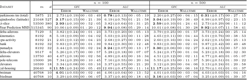
Table 1: To facilitate the comparison between data sets we have normalized the outputs so that their range is one. The accuracy of the algorithms is measured using the root mean squared error, multiplied by100to mimic percentage error (w.r.t. the range of the outputs). The mean and standard deviation of the error are computed after performing10-fold cross-validation. The reported walltime is the average time it takes a method to cross-validate one fold. To assess whether a method performs statistically significantly better than the other on a particular data set we perform the paired Welch t-test [29] withp= 0.05. The significantly better results for the considered settings are marked in bold.
DATASET m d
n= 100 n= 500
GFC ALC GFC ALC
ERROR WALLTIME ERROR WALLTIME ERROR WALLTIME ERROR WALLTIME
parkinsons tm (total) 5875 21 2.73(±0.19)00 : 03 : 49 0.78(±0.13)00 : 05 : 19 2.20(±0.27)00 : 04 : 15 0.31(±0.17)00 : 27 : 15
ujindoorloc (latitude) 21048 527 3.17(±0.15)00 : 21 : 39 6.19(±0.76)01 : 21 : 58 3.04(±0.19)00 : 36 : 49 6.99(±0.97)02 : 23 : 15
ct-slice 53500 380 2.93(±0.10)00 : 52 : 05 3.82(±0.64)03 : 31 : 25 2.59(±0.10)01 : 24 : 41 2.73(±0.29)06 : 11 : 12
Year Prediction MSD515345 90 10.06(±0.09)01 : 20 : 12 9.94(±0.08)05 : 29 : 14 10.01(±0.08)01 : 30 : 28 9.92(±0.07)11 : 58 : 41
delta-ailerons 7129 5 3.82(±0.24)00 : 01 : 23 3.73(±0.20)00 : 05 : 13 3.79(±0.25)00 : 01 : 57 3.73(±0.24)00 : 25 : 14
kinematics 8192 8 5.18(±0.09)00 : 04 : 02 5.03(±0.23)00 : 11 : 28 4.65(±0.11)00 : 04 : 44 5.01(±0.76)00 : 38 : 53
cpu-activity 8192 21 2.65(±0.12)00 : 04 : 23 2.68(±0.27)00 : 09 : 24 2.60(±0.16)00 : 04 : 24 2.62(±0.15)00 : 25 : 13
bank 8192 32 9.83(±0.27)00 : 01 : 39 9.84(±0.30)00 : 12 : 48 9.83(±0.30)00 : 02 : 01 9.87(±0.42)00 : 49 : 48
pumadyn 8192 32 3.44(±0.10)00 : 02 : 24 3.24(±0.07)00 : 13 : 17 3.30(±0.06)00 : 02 : 27 3.42(±0.15)00 : 57 : 33
delta-elevators 9517 6 5.26(±0.17)00 : 00 : 57 5.28(±0.18)00 : 07 : 07 5.24(±0.17)00 : 01 : 04 5.23(±0.18)00 : 32 : 30
ailerons 13750 40 4.67(±0.18)00 : 02 : 56 4.89(±0.43)00 : 16 : 34 4.51(±0.12)00 : 02 : 11 4.77(±0.40)01 : 05 : 07
pole-telecom 15000 26 7.34(±0.29)00 : 10 : 45 7.16(±0.55)00 : 20 : 34 5.55(±0.15)00 : 11 : 37 5.20(±0.51)01 : 39 : 22
elevators 16599 18 3.34(±0.08)00 : 03 : 16 3.37(±0.55)00 : 21 : 20 3.12(±0.20)00 : 04 : 06 3.13(±0.24)01 : 20 : 58
cal-housing 20640 811.55(±0.24)00 : 05 : 49 12.69(±0.47)00 : 11 : 1411.17(±0.25)00 : 06 : 16 12.70(±1.01)01 : 01 : 37
breiman 40768 10 4.01(±0.03)00 : 02 : 46 4.06(±0.04)00 : 13 : 52 4.01(±0.03)00 : 03 : 04 4.03(±0.03)01 : 04 : 16
friedman 40768 10 3.29(±0.09)00 : 06 : 07 3.37(±0.46)00 : 18 : 43 3.16(±0.03)00 : 07 : 04 3.25(±0.09)01 : 39 : 37
An extensive summary containing the results of experiments with the random Fourier features approach (corresponding to Gaussian, Laplace, and Cauchy kernels) and different configurations of á la carte is provided in AppendixD. As the best performing configuration of á la carte on the development data sets is the one withQ= 5components, we report in Table1the error and walltime for this configuration. From the walltime numbers we see that our approach is in both considered settings – with100and500features – always faster than á la carte. Moreover, the proposed approach is able to generate a feature representation with500features in less time than required by á la carte for a representation of100features. In order to compare the performance of the two methods with respect to accuracy, we use the Wilcoxon signed rank test [30,11]. As our approach with500features is on all data sets faster than á la carte with100features, we first compare the errors obtained in these experiments. For95%confidence, the threshold value of the Wilcoxon signed rank test with16data sets isT = 30and from our results we get the T-value of28. As the T-value is below the threshold, our algorithm can with95%confidence generate in less time a statistically significantly better feature representation than á la carte. For the errors obtained in the settings where both methods have the same number of features, we obtain the T-values of60and42. While in the first case for the setting with100features the test is inconclusive, in the second case our approach is with80%confidence statistically significantly more accurate than á la carte. To evaluate the performance of the approaches on individual data sets, we perform the paired Welch t-test [29] withp= 0.05. Again, the results indicate a good/competitive performance of our algorithm compared to á la carte.
4
Discussion
In this section, we discuss the advantages of the proposed method over the state-of-the-art baselines in learning fast shift-invariant kernels and other related approaches.
features are also simple to implement and can be re-trained efficiently with the increase in the number of features [10]. Á la carte, on the other hand, is less flexible in this regard – due to the number of hyperparameters and the complexity of gradients it is not straightforward to implement this method. Scalability. The fact that our greedy descent can construct a feature in time linear in the number of instancesmand dimension of the problemdmakes the proposed approach highly scalable. In particular, the complexity of the proposed parallelization scheme is dominated by the cost of fitting a linear model and the whole algorithm runs in timeO T n3+n2m+nmd, whereTdenotes the number of data passes (i.e., linear model fits) andnnumber of constructed features. To scale this scheme to problems with millions of instances, it is possible to fit linear models using the parallelized stochastic gradient descent [32]. As for the choice ofT, the standard setting in simulations of stochastic gradient descent is5-10data passes. Thus, the presented approach is quite robust and can be applied to large scale data sets. In contrast to this, the cost of performing a gradient step in the hyperparameter optimization of á la carte isO n3+n2m+nmd
. In our empirical evaluation using an implementation with10random restarts, the approach needed at least20steps per restart to learn an accurate model. The required number of gradient steps and the cost of computing them hinder the application of á la carte to large scale data sets. In learning with random Fourier features which also run in timeO n3+n2m+nmd
, the main cost is the fitting of linear models – one for each pair of considered spectral and regularization parameters.
Other approaches.Beside fast kernel learning approaches, the presented method is also related to neural networks parameterized with a single hidden layer. These approaches can be seen as feature construction methods jointly optimizing over the whole feature representation. A detailed study of the approximation properties of a hypothesis space of a single layer network with the sigmoid ridge function has been provided by Barron [4]. In contrast to these approaches, we construct features incrementally by fitting residuals and we do this with a set of non-monotone ridge functions as a dictionary of features. Regarding our generalization bound, we note that the past work on single layer neural networks contains similar results but in the context of monotone ridge functions [1].
As the goal of our approach is to construct a feature space for which linear hypotheses will be of sufficient capacity, the presented method is also related to linear models working with low-rank kernel representations. For instance, Fine and Scheinberg [14] investigate a training algorithm forSVMs using low-rank kernel representations. The difference between our approach and this method is in the fact that the low-rank decomposition is performed without considering the labels. Side knowledge and labels are considered by Kulis et al. [22] and Bach and Jordan [3] in their approaches to construct a low-rank kernel matrix. However, these approaches are not selecting features from a set of ridge functions, but find a subspace of a preselected kernel feature space with a good set of hypothesis. From the perspective of the optimization problem considered in the greedy descent (Algorithm1) our approach can be related to single index models (SIM) where the goal is to learn a regression function that can be represented as a single monotone ridge function [19,18]. In contrast to these models, our approach learns target/regression functions from the closure of the convex hull of ridge functions. Typically, these target functions cannot be written as single ridge functions. Moreover, our ridge functions do not need to be monotone and are more general than the ones considered inSIMmodels. In addition to these approaches and considered baseline methods, the presented feature construction approach is also related to methods optimizing expected loss functions using functional gradient descent [23]. However, while Mason et al. [23] focus on classification problems and hypothesis spaces with finiteVCdimension, we focus on the estimation of regression functions in spaces with infinite VCdimension (e.g., see Section2.2). In contrast to that work, we provide a convergence rate for our approach. Similarly, Friedman [15] has proposed a gradient boosting machine for greedy function estimation. In their approach, the empirical functional gradient is approximated by a weak learner which is then combined with previously constructed learners following astagewisestrategy. This is different from thestepwisestrategy that is followed in our approach where previously constructed estimators are readjusted when new features are added. The approach in [15] is investigated mainly in the context of regression trees, but it can be adopted to feature construction. To the best of our knowledge, theoretical and empirical properties of this approach in the context of feature construction and shift-invariant reproducing kernel Hilbert spaces have not been considered so far.
References
[1] Martin Anthony and Peter L. Bartlett.Neural Network Learning: Theoretical Foundations. Cambridge University Press, 2009.
[2] Nachman Aronszajn. Theory of reproducing kernels.Transactions of the American Math. Society, 1950. [3] Francis R. Bach and Michael I. Jordan. Predictive low-rank decomposition for kernel methods. In
Proceedings of the 22nd International Conference on Machine Learning.
[4] Andrew R. Barron. Universal approximation bounds for superpositions of a sigmoidal function.IEEE Transactions on Information Theory, 39(3), 1993.
[5] Jonathan Baxter. A model of inductive bias learning.Journal of Artificial Intelligence Research, 12, 2000. [6] Alain Bertinet and Thomas C. Agnan.Reproducing Kernel Hilbert Spaces in Probability and Statistics.
Kluwer Academic Publishers, 2004.
[7] Salomon Bochner. Vorlesungen über Fouriersche Integrale. InAkademische Verlagsgesellschaft, 1932. [8] Bernd Carl and Irmtraud Stephani.Entropy, Compactness, and the Approximation of Operators. Cambridge
University Press, 1990.
[9] Felipe Cucker and Steve Smale. On the mathematical foundations of learning.Bulletin of the American Mathematical Society, 39, 2002.
[10] Bo Dai, Bo Xie, Niao He, Yingyu Liang, Anant Raj, Maria-Florina Balcan, and Le Song. Scalable kernel methods via doubly stochastic gradients. InAdvances in Neural Information Processing Systems 27. [11] Janez Demšar. Statistical comparisons of classifiers over multiple data sets.Journal of Machine Learning
Research, 7, 2006.
[12] Michael J. Donahue, Christian Darken, Leonid Gurvits, and Eduardo Sontag. Rates of convex approxima-tion in non-Hilbert spaces.Constructive Approximation, 13(2), 1997.
[13] Rong-En Fan, Kai-Wei Chang, Cho-Jui Hsieh, Xiang-Rui Wang, and Chih-Jen Lin. LIBLINEAR: A library for large linear classification.Journal of Machine Learning Research, 9, 2008.
[14] Shai Fine and Katya Scheinberg. Efficient SVM training using low-rank kernel representations.Journal of Machine Learning Research, 2, 2002.
[15] Jerome H. Friedman. Greedy function approximation: A gradient boosting machine. The Annals of Statistics, 29, 2000.
[16] Israel M. Gelfand and Sergei V. Fomin.Calculus of variations. Prentice-Hall Inc., 1963.
[17] Marc G. Genton. Classes of kernels for machine learning: A statistics perspective.Journal of Machine Learning Research, 2, 2002.
[18] Sham M. Kakade, Varun Kanade, Ohad Shamir, and Adam T. Kalai. Efficient learning of generalized linear and single index models with isotonic regression. InAdvances in Neural Information Processing Systems 24, 2011.
[19] Adam T. Kalai and Ravi Sastry. The isotron algorithm: High-dimensional isotonic regression. In Proceedings of the Conference on Learning Theory, 2009.
[20] Sathiya Keerthi, Vikas Sindhwani, and Olivier Chapelle. An efficient method for gradient-based adaptation of hyperparameters in SVM models. InAdvances in Neural Information Processing Systems 19, 2006. [21] Andrey N. Kolmogorov and Vladimir M. Tikhomirov.-entropy and-capacity of sets in function spaces.
Uspehi Matematicheskikh Nauk, 14(2), 1959.
[22] Brian Kulis, Mátyás Sustik, and Inderjit Dhillon. Learning low-rank kernel matrices. InProceedings of the 23rd International Conference on Machine Learning, 2006.
[23] Llew Mason, Jonathan Baxter, Peter L. Bartlett, and Marcus Frean. Functional gradient techniques for combining hypotheses. InAdvances in large margin classifiers. MIT Press, 1999.
[24] Sebastian Mayer, Tino Ullrich, and Jan Vybiral. Entropy and sampling numbers of classes of ridge functions.Constructive Approximation, 42(2), 2015.
[25] Tom M. Mitchell.Machine Learning. McGraw-Hill, 1997.
[26] Ali Rahimi and Benjamin Recht. Random features for large-scale kernel machines. InAdvances in Neural Information Processing Systems 20.
[27] Walter Rudin.Functional Analysis. Int. Series in Pure and Applied Mathematics. McGraw-Hill Inc., 1991. [28] Luís Torgo. Repository with regression data sets. http://www.dcc.fc.up.pt/~ltorgo/
Regression/DataSets.html, accessed September 22, 2016.
[29] Bernard L. Welch. The generalization of student’s problem when several different population variances are involved.Biometrika, 34(1/2), 1947.
[30] Frank Wilcoxon. Individual comparisons by ranking methods.Biometrics Bulletin, 1(6), 1945.
[31] Zichao Yang, Alexander J. Smola, Le Song, and Andrew G. Wilson. Á la carte—Learning fast kernels. In Proceedings of the 18th International Conference on Artificial Intelligence and Statistics, 2015.
A
Preliminaries
Definition A.1. A symmetric functionk:X×X →Ris a positive definite kernel onXif, for all
n∈N,x1, . . . , xn ∈X, andc1, . . . , cn∈R, it follows thatPni,j=1cicjk(xi, xj)≥0.
Definition A.2. LetD ⊂Rd be an open set. A positive definite kernelk:D×D →Ris called
shift-invariant if there exists a functions:D→Rsuch thatk(x, y) =s(x−y), for allx, y∈D.
The functionsis said to be of positive type.
Definition A.3. A reproducing kernel Hilbert spaceHon a non-empty setX is the Hilbert space of functionsf:X →Rsuch that there exists a unique elementex∈ Hsatisfying the reproducing propertyf(x) =hf,exiHfor allf ∈ H. For a reproducing kernel Hilbert spaceHthe function
k(x, y) = ex(y)is a positive definite kernel. A unique reproducing kernel Hilbert space Hk corresponds to every positive definite kernelk[2].
Theorem A.1. [Bochner, 7] The Fourier transform of a bounded positive measure on Rd is a
continuous function of positive type. Conversely, any function of positive type is the Fourier transform of a bounded positive measure.
In other words, for a shift-invariant kernelkit holds
k(x, y) =s(x−y) = Z
Rd
exp (−ihw, x−yi) dµ(w),
whereµis a positive and bounded measure. Ask(x, y)is a real function in both arguments, the complex part in the integral on the right hand-side is equal to zero, and we have
k(x, y) = 2 Z
cos w>x+b
cos w>y+b
dˆµ(w, b),
whereb∼ U[−π,π]andµˆ(w, b) =µ(w)/2π. Hence, the kernel value at(x, y)can be approximated by
the Monte-Carlo estimate of the dot product [26].
Proposition A.2. [Cucker and Smale, 9] LetKbe a convex and compact subset ofC(X). Then there exists a function inC(X)with a minimal distance tofρinL2ρ(X). Moreover, this function is unique as an element ofL2
ρ(X).
Proof. From the compactness of the subspace it follows that a minimizer exists. However, it does not have to be unique. Letf1andf2be two minimizers and lets={αf1+ (1−α)f2|0≤α≤1}be
the line segment connecting these two points. As the subspaceKis convex, then the segmentsis contained withinK. Furthermore, for allf ∈ s, it holdskf1−fρkρ =kf2−fρkρ ≤ kf−fρkρ.
From the first inequality we have
hfρ−f1, f−f1iρ+hfρ−f1, fρ−fiρ ≤ kfρ−fk 2
ρ⇒ hfρ−f1, f−f1iρ≤ hf1−f , fρ−fiρ.
Similarly, from the second inequality we get
hfρ−f2, f−f2iρ≤ hf2−f , fρ−fiρ.
As the cosine is decreasing function over[0, π], it follows that∠fρf1f ≥∠fρf f1and∠fρf2f ≥
∠fρf f2for allf ∈s. Hence, iff16=f2then the angles∠fρf1fand∠fρf2f are obtuse. As there
does not exist a triangle with two obtuse angles, this is impossible andf1=f2.
Proposition A.3. [Cucker and Smale, 9] Letf1, f2∈ C(X),M ∈R+, and|fi(x)−y| ≤M on a setU ⊂Z of full measure fori= 1,2. Then for allz∈UmfunctionsEρandEzare Lipschitz
continuous on the metric spaceC(X).
Proof. We have that
(f1(x)−y)
2
−(f2(x)−y) 2
Definition A.4. The space is called centralizable if in it, for any open setUof diameter2d, there exists a pointx0from which any pointxis at a distance no greater thand.
Theorem A.4. [Kolmogorov and Tikhomirov, 21] LetSbe a connected totally bounded set which is contained in a centralizable space and letLip1(S)be a set of bounded1-Lipschitz continuous functions onS. If all functions fromLip1(S)are bounded by a constantC >0, then it holds
N(Lip1(S), ,k·k∞)≤2N(S,2,k·k2)
2 2C + 1 .
Proof. As the setSis totally bounded, then for all > 0 there exists a finite-cover ofS. Let
{U}ni=1denote the2-cover of the setSand letxibe the center of the setUi. Letf ∈Lip1(S)and
ˆ
f be an approximation off. Definefˆover the setU1as the number
l2f(x
1)
m
2. Then, for allx∈U1
f(x)−
ˆ
f(x) =
f(x)−
ˆ
f(x1)
≤
f(x)−f(x1) +
2 ≤.
Settingx=x1we see that
f(x1)− ˆ
f(x1)
≤
2.
On the other hand, for the center of the setUithat is adjacent toU1,Ui∩U16=∅, it holds
f(xi)− ˆ
f(x1)
≤ |f(xi)−f(x1)|+
f(x1)− ˆ
f(x1)
≤ 2 +
2 =.
This means that knowing the value at the center ofU1with precision2suffices to approximate with
precisionthe value at the centers of neighbouring sets in the cover. From here it follows that by takingfˆ(x) = ˆf(x1)±2 for allx∈Ui, such thatU1andUiare adjacent, we can approximate
f(xi)− ˆ
f(xi)
with precision
2. As the spaceSis connected it is possible to connect any two
non-adjacent setsUiandUjby a sequence of intersecting setsUk. Hence, we can construct the entire
functionalfˆin this way and approximate the functionf such that f− ˆ f ∞≤.
Now, covering the range of these functions,[−C, C], with-intervals we see that it is sufficient to take 2l2Cm+1numbers as the center-values atx1. For each of the sets in the 2-cover we have two choices
and thus the-covering number ofLip1(S)is not greater than2N(S,2,k·k) 22C
+ 1
.
Theorem A.5. [Cucker and Smale, 9] LetK be a compact and convex subset ofC(X)and let
M >0be a finite constant such that for allf ∈ K,|f(x)−y| ≤M almost everywhere. Then, for
all >0,
Pz∈Zm[Eρ(fz)− Eρ(fK)≤]≥1− N
K,
24M,k·k∞
exp− m
288M2
,
wherefzandfKare the minimizers ofEzandEρoverK.
On the other hand, for the approximation over a compact space only, the following theorem holds. Theorem A.6. [Cucker and Smale, 9] LetKbe a compact subset ofC(X)and letM >0be a finite constant such that, for allf ∈ K,|f(x)−y| ≤M almost everywhere. Then, for all >0,
Pz∈Zm
" sup
f∈K
|Eρ(f)− Ez(f)| ≤
#
≥1−2NK,
8M,k·k∞
exp − m
2
4 2σ2+1 3M
2 !
,
whereσ2= supf∈KVarρ
h
(f(x)−y)2i.
Proposition A.7. [Carl and Stephani, 8] LetEbe a finite dimensional Banach space and letBRbe the ball of radiusRcentered at the origin. Then, ford= dim(E)
N(BR, ,k·k)≤
4R
d
B
Proofs
Theorem 1. Let Hk be a reproducing kernel Hilbert space corresponding to a continuous shift-invariant and positive definite kernelkdefined on a compact setX. Letµbe the positive and bounded spectral measure whose Fourier transform is the kernelk. For any probability measureρdefined onX, it is possible to approximate any bounded functionf ∈ Hkusing a convex combination ofn ridge-wave functions fromFcossuch that the approximation error ink·kρdecays with rateO(1/
√ n).
Proof. Letf ∈ Hk be any bounded function. From the definition ofHk it follows that the set
H0= span{k(x,·)|x∈X}is a dense subset ofHk. In other words, for every >0there is a
bounded functiong∈ H0such thatkf −gkHk< .
As feature functionsk(x,·)are continuous and defined on the compact setX, they are also bounded. Thus, we can assume that there exists a constantB >0such thatsupx,y∈X|k(x, y)|< B. From
here it follows
kf−gk∞= sup
x∈X
hf −g, k(x,·)iH
k
≤
√
Bkf −gkH
k.
This means that convergence ink·kH
kimplies the uniform convergence. The uniform convergence,
on the other hand, implies the convergence inL2
ρnorm, i.e., for any probability measureρon the set
X, for any >0, and for anyf ∈ Hkthere existsg∈ H0such that
kf−gkρ< . (1)
The functiongis by definition a finite linear combination of feature functionsk(xi,·)[see, e.g.,
Chapter 1 in6] and by TheoremA.1it can be written as
g(x) =
l
X
i=1
αik(xi, x) = 2
Z l X
i=1
αicos w>xi+b
!
cos w>x+b
dˆµ(w, b)
= 2µ(0) Z
u(w, b) cos w>x+bd˜µ(w, b),
where µ˜ is a probability measure on Rd ×[−π, π], u(w, b) = Pli=1αicos w>xi+b
, and R
dˆµ(w, b) = µ(0) < ∞. From the boundedness of g, it follows that the function u is bounded for all w andb from the support of µ˜, i.e., |u(w, b)| ≤ Pl
i=1|αi| < ∞. Denoting
withγ(w, b) = 2µ(0)u(w, b), we see that it is sufficient to prove that Eµ˜(w,b)
γ(w, b) cos w>x+b
∈co (Fcos),
where the closure is taken with respect to the norm inL2ρ(X). In particular, for a sample(w,b) =
{(wi, bi)} s
i=1drawn independently fromµ˜we have
E(w,b)
Z
g(x)−1 s
s
X
i=1
γ(wi, bi) cos wi>x+bi
!2 dρ = 1 s2 Z E(w,b)
s X i=1
g(x)−γ(wi, bi) cos w>i x+bi
| {z }
ξ(x;wi,bi)
2
dρ=
1
s2
Z E(w,b)
s
X
i=1
ξ(x; wi, bi)
!2 dρ=
1
s
Z Eµ˜
h
ξ(x; w, b)2idρ=
1
s
Z Varµ˜
g(x)−γ(w, b) cos w>x+bdρ= 1
s
Z Varµ˜
γ(w, b) cos w>x+bdρ.
Note that the third equation follows from the fact thatξ(x; wi, bi)are independent and identically
distributed random variables andE[ξ(x; wi, bi)ξ(x; wj, bj)] = 0. As established earlier,
coeffi-cientsγ(w, b)are bounded and, therefore, random variableηx(w, b) =γ(w, b) cos w>x+b
bounded, as well. Hence, fromsupw,b|ηx(w, b)|=D <∞it follows thatVarµ˜(ηx(w, b))≤D2
and consequently forgs(x; (w,b)) = 1sP s
i=1γ(wi, bi) cos w>i x+bi
we get
Egs
h
kg−gsk 2 ρ
i
≤D
2
s . (2)
As the expected value of the normkg−gskρis bounded by a constant, it follows that there exists
a functiongswhich can be represented as a convex combination ofsridge-wave functions from
Fcosand for which it holdskg−gskρ∈ O
1
√ s
. Moreover, there exists a sequence of functions
{gn}n≥1converging togink·kρsuch that eachgnis a convex combination ofnelements fromFcos
andkg−gnkρ ∈ O
1
√ n
.
Hence, we have proved thatg∈co (Fcos), where the closure is taken with respect tok·kρ. It is then
possible to approximate any bounded functionf ∈ Hkusing a convex combination ofnridge-wave
functions fromFcoswith the rateO
1
√ n
, i.e., for alln∈N
kf−gnkρ≤ kf−gkρ+kg−gnkρ∈ O
1
√ n
.
Proposition 2. For any Hilbert space the modulus of smoothness is equal toτ(r) =√1 +r2−1. Proof. Expanding norms using the dot product we get
2 (τ(r) + 1) = sup kfk=kgk=1
p
1 +r2+ 2rhf, gi+p1 +r2−2rhf, gi.
Denoting withu = 1 +r2 andv = 2rhf, giand using the inequality between arithmetic and
quadratic mean we get
√
u+v+√u−v≤2
r
u+v+u−v
2 = 2
√ u.
As the equality is attained forv= 0it follows that the modulus of smoothness of a Hilbert space is given by
τ(r) =p1 +r2−1.
Corollary 4. Let{fn}n≥1⊂co (FΘ)be an-greedy incremental sequence of functions constructed according to the procedure described in Theorem3with respect to a functionf ∈co (FΘ). Then, it
holdskfn−fkρ≤
(K+)√2+log2n/2n
√
n .
Proof. AsL2
ρ(X)is a Hilbert space, it follows from Proposition2that the modulus of smoothness
of this space isτ(r) = √1 +r2−1. While it is straightforward to show that√1 +r2 ≤1 +r
forr ∈R+0, this bound is not tight enough asr→0. A tighter upper bound for this modulus of
smoothness can be derived from the inequality√1 +r2≤1 +r2
2. To see that this is a better bound
for the case whenr→0, it is sufficient to check that1 +r22 ≤1 +rfor all0≤r≤2. Hence, all conditions of Theorem3are satisfied and the claim follows by takingt= 2andγ= 12. Proposition 5. The hypothesis spaceFis a convex and compact subset of the metric spaceC(X). Moreover, the elements of this hypothesis space are Lipschitz continuous functions.
Proof. Letf, g∈ F. As the hypothesis spaceFis the closure of the convex hull,co (FΘ), it follows
sufficiently largenit holdskf−fnk∞< andkg−gnk∞< . Then, for a convex combination of
functionsf andgand sufficiently largenwe have
kαf+ (1−α)g−αfn−(1−α)gnk∞≤αkf−fnk∞+ (1−α)kg−gnk∞< .
From here it follows that for every0≤α≤1andf, g∈ Fit holdsαf+ (1−α)g∈ F. Thus, we have showed that the hypothesis spaceFis a convex set.
As a convex combination of Lipschitz continuous functions is again a Lipschitz continuous function, we have that all functionsf ∈co (FΘ)are Lipschitz continuous. It remains to prove that all functions
from the closure are Lipschitz continuous, as well. Letfand{fn}n≥1be defined as above and let
Lφbe the Lipschitz constant of the functionφ. We have that it holds
|f(x)−f(y)| ≤ |f(x)−fn(x)|+|fn(x)−fn(y)|+|fn(y)−f(y)|<
2kf −fnk∞+rLφkx−yk.
Taking the limit of both sides asn→ ∞, we deduce that functionf is Lipschitz continuous with a Lipschitz constant bounded byrLφ.
Depending on the choice of the basis functionφ, the hypothesis space can be a space of infinite dimension and the fact that it is bounded and complete does not imply that it is compact, as well. The metric space(F,k·k∞)is compact if and only if it is complete and totally bounded [27], i.e., for
all >0there exists a finite-net ofF. As the hypothesis spaceF is complete by definition, it is
sufficient to show that for all >0there exists a finite-net ofFinC(X). The setXis a compact subset of finite dimensional Euclidean space and as such it is totally bounded and contained in a centralizable space (see DefinitionA.4for details). Then, from TheoremA.4it follows that
N(Lip1(X), ,k·k∞)≤2 N(X,
2,k·k)
2
2C
+ 1
,
whereLip1(X)denotes the set of1-Lipschitz functions defined on a setX,N(X, ,k·k)denotes the minimal number of points in an-net of the setX with respect to the metrick·k, andC >0is the upper bound on all functions inLip1(X). This result allows us to bound the covering number of the
space of Lipschitz continuous functions on the compact setX. Namely, from the assumptions about
Fwe conclude that all functions inFhave Lipschitz constant bounded byLF =rLφ, whereLφ
denotes the Lipschitz constant of the functionφ. Then, the upper bound on the covering number of the spaceLipLF(X)is given by
2N
X,
2LF,k·k2
2
2r
+ 1
.
SinceF ⊂LipLF(X)andN LipLF(X), ,k·k∞
is finite, the result follows.
Theorem 6. LetM >0such that, for allf ∈ F,|f(x)−y| ≤M almost surely. Then, for all >0 P[Eρ(fz)− Eρ(f∗)≤]≥1− N(F,/24M,k·k∞) exp (−m/288M2),
wherefzandf∗are the minimizers ofEzandEρon the setF,z∈Zm, andN(F, ,k·k∞)denotes the-covering number ofFw.r.t.C(X).
Proof. The claim follows from Proposition5and TheoremA.5.
Corollary 7. For all > 0and allδ > 0, with probability1−δ, a minimizer of the empirical squared error on the hypothesis spaceF is(, δ)-consistent when the number of samples m ∈
Ω r(Rs+t)Lφ12 + 1 ln
1 δ
.Here,Ris the radius of a ball containing the set of instancesXin its interior,Lφis the Lipschitz constant of a functionφ, andr,s, andtare hyperparameters ofFΘ.
Proof. To derive a sample complexity bound from the corollary we need a tighter bound on the covering number of our hypothesis space than the one provided in Proposition5. We first give one such bound and then prove the corollary.
in its interior. From the definition of the hypothesis spaceFwe see that the argument of the ridge functionφis bounded, i.e.,
|hw, xi+b| ≤ kwk kxk+t≤Rs+t.
From here we conclude that the hypothesis spaceFis a subset of the space of1-dimensional Lipschitz continuous functions on the compact interval[−(Rs+t), Rs+t]. Then, the covering number ofF
is upper bounded by the covering number of the space ofLF-Lipschitz continuous one dimensional functions defined on the segment[−(Rs+t), Rs+t].
From PropositionA.7it follows that the-covering number of the segment[−(Rs+t), Rs+t]is upper bounded by4(Rs+t). This, together with TheoremA.4implies that the upper bound on the
-covering number of the hypothesis spaceFis given by
N(F, ,k·k∞)≤2
8r(Rs+t)Lφ
2
2r
+ 1
. (3)
On the other hand, from Theorem6we get that for allδ >0with probability1−δthe empirical estimator is(, δ)-consistent when
2
192r(Rs+t)M Lφ
2
48M r
+ 1
exp− m
288M2
≤δ,or 192r(Rs+t)M Lφ
ln 2 + ln
2
48M r
+ 1
≤ m
288M2 −ln
1
δ.
Hence, for all, δ >0and
m≥288M
2
"
192r(Rs+t)M Lφ
ln 2 + ln
2
48M r
+ 1
+ ln1
δ
#
(4)
with probability1−δthe empirical estimator is(, δ)-consistent.
Remark 1. The concentration inequality is tighter by a factor of1for convex and compact compared to compact only hypothesis spaces. For instance, this can be seen by comparing the bounds from TheoremsA.5andA.6. In our case with convex and compact hypothesis spaceF, the final sample complexity bound is stillΩ 1
2
due to the 1 factor coming from the-covering number ofF.
C
Implementation Details
In this appendix, we provide implementation details for all the considered algorithms – greedy feature construction, á la carte method [31], and random Fourier features approach [26]. As already stated in Section2.5, the corresponding linear ridge regression optimization problems are solved by casting them as hyperparameter optimization problems [20]. To be as objective as possible to the best performing competing method [31], we have followed the experimental setting outlined there and optimized the hyperparameters with theL-BFGS-Bsolver fromSciPy.
C.1 Greedy Feature Construction
We have implemented a distributed version of Algorithm2using a python packagempi4py. For the experiments with100spectral features the algorithm is simulated using5cores on a single physical machine – each core corresponds to one instance of greedy functional descent. The remaining parameters are: the number of data passesT = 1, the maximum number of greedy descent steps
p= 20, precision parameter= 0.01that stops the greedy descent when the successive improvement in the accuracy is less than1%, and feature cut-offηthat is set to0.0001%of the range of the output variable. For the experiments with500spectral features the algorithm is simulated using5physical machines. To communicate features more efficiently5cores on each of the physical machines is used giving the total number of25cores corresponding to25instances of greedy functional descent. The remaining parameters for this setting are identical to the ones used in the experiments with 100features. As the greedy functional descent is stopped when the successive improvement in the accuracy is below1%, the approach terminates sooner than the alternative approaches (w.r.t. the number of constructed features) for simple hypotheses (see AppendixD). In contrast to á la carte [31], wedid not engineer a heuristic for the initial solutionof the hyper-parameter optimization problem. Instead, we have initialized the spectral features by sampling from the standard normal distribution and dividing the entries of the sampled vector with the square root of its dimension.
Having specified the parameter settings for Algorithm2, we proceed to a discussion regarding the regularization term from the optimization problem defined at line3of Algorithm1. The section concludes with hyperparameter gradients for the cosine-wave feature space introduced in Section2.2. Regularization. It is frequently the case that generalization properties and the capacity of a hy-pothesis space are controlled by penalizing the objective function with the squaredl2norm of a
parameter vector. For instance, this is the case for the majority of standard activation functions in neural networks literature. The reason behind this choice of the regularizer lies in the fact that these activation functions are monotone and the variation of any such basis function corresponds with the variation in its ridge argument. Assuming that the data is centered, the variation of the ridge argument can be expressed as
Z
w>xx>wρ(x) =w>
Z
xx>ρ(x)
w=kwk2.
However, if we opt for cosine ridge functions as in Sections2.2and3, then it is not straightforward to relate the smoothness of the basis function to its argument (considered over a given finite sample of the data). Namely, cosine is a periodic function and while spectral parameters with large norms can cause significant variation in the ridge argument, this does not necessarily imply a large variation of the basis function over a finite sample. It is also possible for a parameter vector with the smaller norm to cause more variation in the basis function over a finite sample than the one with the larger norm. We, therefore, opt to regularize the spectrum of the cosine ridge function by penalizing the objective with its squaredL2
ρ(X)norm. Before we give the regularization term, we first note that the
bias term from the cosine-wave features can be eliminated using the trigonometric additive formulas and then the cosine-wave basis function takes the from
φw,a(x) =a1sin w>x
+a2cos w>x
. (5)
Now, taking the squaredL2
ρ(X)norm of this function we get
kφw,ak 2
ρ =a
2 1
Z
sin2 w>xρ(x) +a22
Z
cos2 w>xρ(x) +a1a2
Z
sin 2w>xρ(x)
=a
2 1+a22
2 +
a22−a21
2 Z
cos (2r)µw(r) +a1a2
Z
where µw(r) =
R
ρ x|w>x=r. If we assume that the probability measure ρis symmetric, then we have thatµw(r) =µw(−r)and using the fact thatsin (2r)is an odd function, we obtain
R
sin 2w>x
ρ(x) = 0. In the absence of the marginal distributionρ, the integralR cos (2r)µw(r)
can be estimated from the training sample with m1 Pm
i=1cos 2w
>x i
, wherexi i.i.d.
∼ ρ(x).
Hyper-parameter optimization.We now formulate the optimization problem (line3, Algorithm1) for the setting with cosine-wave features and provide the gradients for all the hyperparameters. The optimization problem can be specified as
min 1
m
m
X
i=1
c0f0,i+c1sin w>xi+c2cos w>xi−yi 2 + λ c 2 0 m m X i=1
f02,i+c
2 1+c22
2 +
c2 2−c21
2m
m
X
i=1
cos 2w>xi+
2c0c1
m
m
X
i=1
sin w>xif0,i+
2c0c2
m
m
X
i=1
cos w>xi
f0,i+
c1c2
m
m
X
i=1
sin 2w>xi
!
,
where wandλare optimized as hyperparameters and amplitude vectorcas a regressor. As the regressor is completely determined by the choice ofλ, it is sufficient to optimize this problem only by the hyperparameterswandλ. We want to choose these parameters viak-fold cross-validation and in order to achieve this we follow the procedure proposed by Keerthi et al. [20]. Let us denote the above described3-dimensional feature representation of the data with Zw ∈ Rm×3 and setσ0 = m1
Pm
i=1f 2
0,i,σ1 = m1
Pm
i=1sin w
>x i
f0,i,σ2 = m1
Pm
i=1cos w
>x i
f0,i,σ3 = 1
m
Pm
i=1sin 2w
>x i
,σ4= m1 P m
i=1cos 2w
>x i
. Now, in the place of the identity matrix in the derivative of the ridge regression objective function we have the matrix
D=
" σ
0 σ1 σ2
σ1 0.5 (1−σ4) 0.5σ3
σ2 0.5σ3 0.5 (1 +σ4)
#
At this point our derivation follows closely the derivation by Keerthi et al. [20]. Taking the derivatives with respect tocand setting the gradient of the loss to zero we get
Zw>Zwc−Zw>y+mλDc= 0,
Zw>Zw+mλD
c=Zw>y.
Let us now denote withP =Zw>Zw+mλD,q=Zw>y, andθ= (w, λ). We note here thatP andq
are defined over thetraining instancesxand their labelsy. We now take the implicit derivative of this equation to obtain the derivative of the regressorcwith respect to the hyperparameters, i.e.,
∂c
∂θ =P
−1 ∂q ∂θ− ∂P ∂θc .
As already stated, the choice ofλdirectly determines the coefficientscand to obtain these we need to perform the hyperparameter selection which is done over the validation samples. In other words,
θ∗= arg min
θ 1 k k X i=1 1
|Fi|
X
(x,y)∈Fi
c>zw(x)−y
2
,
where Fi denotes one of k validation folds in the k-fold cross-validation and zw(x) is the
3-dimensional representation of an instancex ∈ X. Let us now consider only the sample from one validation fold and denote it withF. At the same time letFcdenotes its complement or the training sample whenFis used as the validation fold. Here, we note that(x, y)∈F aredifferent
from samples participating in the definitions ofP andqwhen takingFas the validation fold. Taking derivatives with respect toθwe get the hyperparameter gradient
2
|F|
X
(x,y)∈F
c>zw(x)−y
∂z
w(x)
∂θ c+zw(x)P
Let us introduce a vectort= (t0, t1, t2)as a solution to the following3-dimensional linear system
P t= 1
|F|
X
(x,y)∈F
c>zw(x)−y
zw(x).
We then write the derivative of each term in the hyperparameter gradient separately as
∂
∂w c
>z
w(x)= c1cos w>x−c2sin w>xx
∂
∂w t
>q
= X
(x,y)∈Fc
t1cos w>x−t2sin w>xxy
∂
∂w t
>P c
= (1 +λ) (t0c1+t1c0)
|Fc|
X
i=1
f0,icos w>xi
xi−
(1 +λ) (t0c2+t2c0)
|Fc|
X
i=1
f0,isin w>xi
xi+ (1 +λ) (t1c2+t2c1)
X
x∈Fc
cos 2w>x
x+
(1 +λ) (t1c1−t2c2)
X
x∈Fc
sin 2w>x
x
∂
∂λ =m t
>Dc
Performing the gradient descent using these hyperparameter gradients we obtain both the spectrumw
and the amplitudesc. The spectrum regularization term which is defined using the empirical estimates of the sine and cosine integrals affects the gradient with respect towvia theλfactor in the third expression. In our experiments, we have observed that the capacity parameterλusually takes the value below10−4. Thus, the influence of the spectrum regularization term is less significant than the
amplitude regularization term. For this reason, in our implementation we only penalize the empirical squared error objective with the squared norm of the amplitude vector, i.e.,Ω (c, w) =kck22. C.2 Random Fourier features
As already pointed out in TheoremA.1and AppendixA, any shift-invariant positive definite kernel can be represented as a Fourier transform of a positive measure. Thus, in order to generate a kernel feature map it is sufficient to sample spectral frequencies from this measure. Genton [17] and Rahimi and Recht [26] have provided the parameterized spectral density functions corresponding to Gaussian, Laplace, and Cauchy kernels. We use these parameterizations to generate spectral features and then train a linear ridge regression model in the constructed feature space. To choose the most suitable parameterization, we cross-validate10parameters from the log-space of[−3,2].
C.3 A la carte
The random Fourier features approach [26] is an efficient method for the approximation of functions from shift-invariant reproducing kernel Hilbert spaces. However, this method requires ana priori
specification of a suitable spectral measure which is often not feasible. To address this shortcoming, Yang et al. [31] estimate a data-dependent spectral distribution using a mixture of Gaussians and represent the regression estimator as
f(x) =
n
X
j=1
αjsin w>jx
+α0jcos wj>x
,
wherendenotes the number of spectral features, and
w∼
Q
X
k=1
γk
q
(2π)d|Σk|
exp −(x−µk)
>
Σ−k1(x−µk)
2
withΣkdiagonal,γ≥0, andP Q
k=1γk = 1. The proposed algorithm finds a feature representation
together with a linear model by optimizing the marginal likelihood of a Gaussian process. As we have chosen to compare all the feature construction approaches using the standard linear regression, we provide an equivalent implementation of this approach based on the hyper-parameter optimization method proposed by Keerthi et al. [20]. To make the comparison as objective as possible, we have parallelized the implementation of this algorithm and simulated it by following theARD-heuristic for choosing the initial solution [31, Supplementary material]. In all the experimental settings (with100 and500features), we have run this algorithm usingQ= 1,Q= 2, andQ= 5mixture components. Optimization problem.We first give the optimization objective for the non-Gaussian process case,
min 1 m m X i=1 " Q X q=1
νq2
s
X
j=1
αqjsin
u>qjΣ1q/2xi+µ>qxi
+βqjcos
u>qjΣ1q/2xi+µ>qxi
−yi
#2 +
λkαk2+kβk2,
where αand β are optimized as regressors andµq, Σq (diagonal covariance matrix), andλas
hyper-parameters. Theu-vectors are random vectors sampled from the multivariate standard normal distribution. These vectors act as a regularization term on the spectrum of the cosine features forcing the frequencies to stay in the pre-specified number of clusters/components.
Hyper-parameter optimization. Let us denoteΣ1q/2 withDq, parameterized features withZθ ∈
Rm×Qs, hyperparameters withθ= (µ, D, ν), and regressors withc= (α, β). Similar to the previous section setP =Zθ>Zθ+mλIandq=Zθ>y. Following the same principles for the implicit derivation,
we obtain the gradient terms of the hyper-parameter objective function:
∂ ∂µq
c>zθ(x)
=νq2
α>q cos UqDqx⊕µ>qx
−βq>sin UqDqx⊕µ>q x
x,
∂
∂Dq
c>zθ(x)
=νq2(αqUq)>cos UqDqx⊕µ>qx
−(βqUq)>sin UqDqx⊕µ>qx
x,
∂ ∂νq
c>zθ(x)= 2νq
α>q sin UqDqx⊕µ>qx
+βq>cos UqDqx⊕µ>qx
,
∂ ∂µq
t>q
= X
(x,y)∈Fc
yνq2t>qαcos UqDqx⊕µ>qx
−t>qβsin UqDqx⊕µ>qx
x,
∂
∂Dq
t>q
= X
(x,y)∈Fc
yνq2(tqαUq) >
cos UqDqx⊕µ>qx
−(tqβUq) >
sin UqDqx⊕µ>qx
x,
∂ ∂νq
t>q = 2νq
X
(x,y)∈Fc
t>qαsin UqDqx⊕µ>q x
+t>qβcos UqDqx⊕µ>qx
,
∂ ∂µq
t>P c
= X
(x,y)∈Fc
νq4
(
"
t>αsin U Dx⊕µ>x
+t>β cos U Dx⊕µ>x #
·
"
α>q cos UqDqx⊕µ>qx
−βq>sin UqDqx⊕µ>qx
#
+
"
α>sin U Dx⊕µ>x
+β>cos U Dx⊕µ>x #
·
"
t>qαcos UqDqx⊕µ>qx
−t>qβsin UqDqx⊕µ>qx
#)
∂ ∂νq
t>P c= 2 X
(x,y)∈Fc
νq3
(
"
t>αsin U Dx⊕µ>x
+t>β cos U Dx⊕µ>x #
·
"
α>sin U Dx⊕µ>x
+β>cos U Dx⊕µ>x #)
∂
∂Dq
t>P c
= X
(x,y)∈Fc
νq4
(
"
t>αsin U Dx⊕µ>x
+t>β cos U Dx⊕µ>x #
·
"
(αqUq) >
cos UqDqx⊕µ>qx
−
(βqUq)>sin UqDqx⊕µ>qx
#
+
"
α>sin U Dx⊕µ>x
+β>cos U Dx⊕µ>x #
·
"
(tqαUq)>cos UqDqx⊕µ>q x
−
(tqβUq)>sin UqDqx⊕µ>qx
#)
x
∂
∂λ =m t
>c,
where⊕anddenote element-wise addition and multiplication,U ∈ RQs×dand it consists of blocksUq ∈Rs×dsuch that each block contains row vectors sampled from a multivariate standard normal distribution.
The cost of computing the gradient of hyperparameters for á la carte involves solving ann=Qs
dimensional linear system. This system needs to be solved for each validation fold in thek-fold splitting, required for the optimization of the hyperparameters over the validation samples. As this can be computationally intensive on a single core, we have parallelized our implementation of á la carte by computing the parts of hyperparameter gradient that correspond to different validation folds on different cores. For the inner cross-validation performed with5-fold splitting this has resulted in a speed up of approximately4-5times compared to a single core implementation. In Section3and AppendixD.1we report the walltimes of the parallelized implementation of á la carte.