An idealised study for the long term evolution
1of crescentic bars
2W.L. Chen,
a,∗
N. Dodd,
aM.C.H. Tiessen,
bD. Calvete
c3
aFaculty of Engineering, University of Nottingham, Nottingham NG7 2RD, UK.
4
bDeltares, Marine and Coastal Systems Unit, Department of Environmental
5
Hydrodynamics, Rotterdamseweg 185, 2629 HD Delft, The Netherlands.
6
cDepartment de F´ısica Aplicada, Universitat Polit`ecnica de Catalunya, Jordi
7
Girona 1-3, E-08034 Barcelona, Spain.
8
Abstract
9
An idealised study that identifies the mechanisms in the long term evolution of 10
crescentic bar systems in nature is presented. Growth to finite amplitude (i.e., equi-11
libration, sometimes referred to as saturation) and higher harmonic interaction are 12
hypothesised to be the leading nonlinear effects in long-term evolution of these sys-13
tems. These nonlinear effects are added to a linear stability model and used to 14
predict crescentic bar development along a beach in Duck, North Carolina (USA) 15
over a 2-month period. The equilibration prolongs the development of bed pat-16
terns, thus allowing the long term evolution. Higher harmonic interaction enables 17
the amplitude to be transferred from longer to shorter lengthscales, which leads to 18
the dominance of shorter lengthscales in latter post-storm stages, as observed at 19
Duck. The comparison with observations indicates the importance of higher har-20
monic interaction in the development of nearshore crescentic bar systems in nature. 21
Additionally, it is concluded that these nonlinear effects should be included in mod-22
els simulating the development of different bed patterns, and that this points a way 23
forward for long-term morphodynamical modelling in general. 24
Key words: Crescentic bed-patterns, linear stability analysis, field observations, 25
long term evolution, nearshore morphology, higher harmonic interaction 26
1 Introduction
27
Nearshore sea bed patterns are a common feature around the world and may
28
provide some protection to beach and coastal areas (Hanley et al., 2014).
29
As one of the most common nearshore sea bed patterns, crescentic bars are
30
observed worldwide, see e.g.Van Enckevort et al.(2004). Such near shore sand
31
bars can reduce wave momentum flux, or radiation stress, as the wave breaking
32
on top of it. Furthermore, it can also provide sand to the beach if it migrates
33
onshore (Ribas et al., 2015b). Because of their prevalence, their possible role
34
in coastal protection, and the need to gain more understanding of nearshore
35
coastal dynamics in general, it is important to study the evolution of these
36
morphological features.
37
Increasingly, the genesis of such quasi-periodic patterns is thought to be due
38
to morphological instability (see Ribas et al., 2015a). An often used method
39
for describing the development of crescentic bed-forms in idealised scenarios is
40
therefore linear stability analysis, see e.g.Deigaard et al.(1999);Falqu´es et al. 41
(2000); Damgaard et al. (2002); Calvete et al. (2005); Van Leeuwen et al.
42
(2006); Calvete et al. (2007). In this method, infinitesimally small
perturba-43
tions are imposed on an equilibrium (basic) state. The interaction of flow and
44
sea bed may give rise to a so called fastest growing mode, a bed-form with
45
largest growth rate, which will dominate the sea bed pattern after a period
46
of evolution. Linear stability analysis has proved to be useful in revealing the
47
initialization and short term evolution of crescentic bars.
48
Following this approach, Tiessen et al. (2010) predicted the development of
49
crescentic bed-patterns at Duck, North Carolina (USA), for a period of two
50
months, starting from an along-shore constant bed. The forcing used was the
51
measured wave and tidal data at the same field site. Although the predicted
52
crescentic pattern lengthscales were similar to those observed, they tended to
53
exhibit a much bigger fluctuation. Such significant discrepancy is found to be a
54
combined result of missing nonlinear effects in the linear model and the effect
55
of pre-existing bed patterns in the natural environment. This is because linear
56
stability analysis is limited when pre-existing bed-forms are present, since an
57
alongshore constant initial bathymetry is assumed at each instant. Another
58
reason is that the exponentially growing bed form will violate the small
am-59
plitude assumption after some time, and nonlinear effects will dominate the
60
evolution thenceforth. Therefore, a nonlinear analysis is necessary for reliable
61
long-term prediction of crescentic bars (Dodd et al., 2003).
62
Using fully nonlinear numerical models, Tiessen et al. (2011) and Smit et al. 63
(2012) included nonlinear effects and investigated the impact of pre-existing
64
bed-patterns. Smit et al. (2012) showed that pre-existing bed-patterns ‘with
65
significant variability’ do not adapt to changed hydrodynamic conditions, and
dominate subsequent development. Moreover, such tendency holds for
increas-67
ing wave energy. This suggests that, under certain circumstances, pre-existing
68
modes are not affected by the present forcing conditions and that once a
cer-69
tain threshold of development is reached, only a reset-event, such as a storm,
70
can remove pre-existing bed-forms and the corresponding dominant crescentic
71
bed-pattern lengthscale.
72
On the other hand, Tiessen et al. (2011) showed that pre-existing modes can
73
modify the subsequent development of different crescentic bar lengthscales.
74
Pre-existing modes (patterns) of finite amplitude will persist if those same
75
modes show significant linear growth (i.e., initial growth from an
infinitesi-76
mally disturbed beach). On the contrary, pre-existing lengthscales that show
77
only limited growth or even decay when developing from an infinitesimally
78
disturbed beach, become overwhelmed by faster growing modes. However, the
79
lengthscale of these pre-existing, slowly growing or decaying modes, and that
80
of the newly-arising crescentic bed-form are linked. This is because the more
81
rapid initial development of higher harmonics of the pre-existing lengthscale
82
can excite a linearly unstable mode at a smaller wavelength, prior to decaying
83
to insignificance.
84
The findings of Tiessen et al. (2011) and Smit et al. (2012) suggested a few
85
important nonlinear effects in the long-term evolution of crescentic bars: higher
86
harmonic interaction, persistence of bed-forms through weak storm and the
87
importance of pre-existing bed-forms. Although the long term development
88
of crescentic bars has been studied by many nonlinear numerical studies (e.g.
89
Garnier et al., 2008; Castelle and Ruessink, 2011; Tiessen et al., 2011; Smit 90
et al., 2012), all the existing nonlinear modelling studies are so far restricted
91
to idealised simplified cases. Therefore, the existing knowledge of important
92
nonlinear effects in the long-term evolution of crescentic bars lacks comparison
93
with observations.
94
The goal of this study is therefore to identify physical mechanisms for
long-95
term growth of crescentic bar systems by comparing with field observations.
96
To this end, we develop an idealised model that incorporates the processes
97
suggested by Tiessen et al. (2011) and Smit et al. (2012) into the linear
sta-98
bility analysis. The occurrence of pre-existing modes is also accounted for in
99
the model. This approach allows us to consider only those effects identified
100
earlier, and, moreover, is time efficient and so can be applied over
substan-101
tial durations. The model is used to predict the lengthscale of the crescentic
102
bed-forms for a period of two months in 1998 at Duck (NC, USA). The model
103
results are compared with field observation (Van Enckevort et al., 2004) over
104
the same period.
105
The paper is organized as follows. In section 2 the model formulation is given,
as well as how linear stability theory is used in the amplitude evolution model.
107
In section 3 the amplitude evolution model is presented, and an example test
108
case used to illustrate its properties. Model results and a discussion are
pre-109
sented in section 4 and 5, respectively. Finally, a conclusion is given in
sec-110
tion 6.
111
2 Model formulation: governing equations and linear stabiity
anal-112
ysis
113
The model geometry describes an unbounded, straight alongshore uniform
114
open coast, with an example of cross-shore profile being shown in Fig. 1.
Quasi-115
steady flow conditions are assumed and the spatial coordinate system, (x, y)
116
in m, is aligned with cross- and long-shore directions. The vertical direction is
117
denoted byz (m), wherez = 0 refers to mean sea level with positive z points
118
upwards.
119
The model-framework is composed of the phase-averaged shallow water
equa-120
tions, in combination with a description of the bathymetric evolution, the
121
wave phase and the wave energy density (see Calvete et al. (2005) for a more
122
extensive description of this model).
123
The equations of the model are:
124 125
∂D ∂t +
∂Duj
∂xj
= 0, (1)
∂ui
∂t +uj ∂ui
∂xj
=−g∂zs ∂xi
− 1
ρD ∂ ∂xj
S
0 ij −S
00 ij
−
τbi
ρD, (2)
∂E ∂t +
∂ ∂xj
((uj +cgj)E) +Sij0
∂uj
∂xi
=−D, (3)
∂Φ
∂t +σ+uj ∂Φ ∂xj
= 0 (4)
∂zb
∂t + 1 1−p
∂qj
∂xj
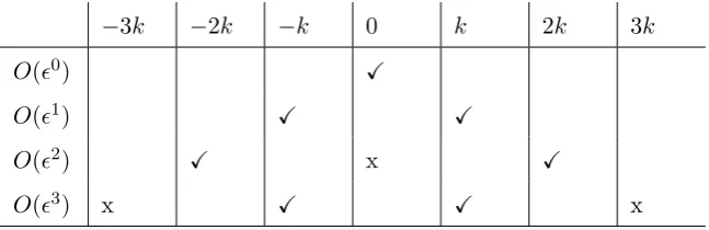
= 0, (5)
where i, j = 1,2, with summation being on j; x1,2 = (x, y) and u1,2 = (u, v),
126
where u and v (ms−1) are the cross- and alongshore depth-averaged current
127
respectively. t(s) represents time. zs(x, y, t) is the mean sea level,zb(x, y, t) is 128
the mean bed level andDis the total mean depth (D=zs−zb).E(x, y, t) (kg 129
s−2) is the wave energy density, which can be expressed in terms of the wave
130
height (E = 18ρgH2
rms). τbi (kg m−1 s−2) represents the bed shear stress; here 131
the expression ofFeddersen et al.(2000) is used.g (m s−2) is the gravitational
acceleration, Φ (rad) is the wave phase and σ (Hz) is the intrinsic frequency.
133
The sediment flux (qi, in kg s−1) is represented by the formula of Soulsby and 134
Van Rijn (Soulsby, 1997). The bed porosity pis 0.4 and the seawater density
135
(ρ) is 1024 kg m−3. Sij0 (kg s−2) is the radiation stress term and Sij00 (kg s−2)
136
represents the Reynolds stresses (Calvete et al., 2005). D (kg s−3) is the wave
137
energy dissipation due to wave breaking described according to Church and
138
Thornton (1993).
139 140
2.1 Linear stability analysis 141
In a linear stability analysis, the variables consist of an alongshore- and time invariant solution of (1)-(5), the basic state, denoted here with a zero sub-script, and a small perturbation to that solution.
{zs, zb, u1, u2, E,Φ}={Zs0(x), Zb0(x),0, V0(x), E0(x),Φ0(x, t)}
+Ψ(x) exp (ωt+ iky). (6)
The basic state corresponds to the wave conditions and water levels
per-142
taining throughout the 2 months at Duck (see §2.2). It contains bed level
143
Zb0, mean water level Zs0, alongshore current V0, wave energy density E0
144
and phase Φ0. The second term on the right hand side of (6) is the
pertur-145
bation. The disturbances considered are alongshore-periodic with arbitrary
146
wavelength λ = 2π/k, and (complex) frequency ω = ωr+ iωi. Thus the real 147
part of the frequency wr represents the growth rate of the periodic pattern, 148
while the imaginary part ωi is related to the corresponding migration rate
149
(cm = −ωi/k). A pattern with positive wr indicates a mode unbounded in 150
time, i.e. a growing mode. The growthrate is determined by the combined
151
effect of wave forcing and bathymetry, and has been studied by Calvete et al. 152
(2005). Among all growing modes, the one with largestωris defined as Fastest 153
Growing Mode (FGM). For a chosen k, the evolution of the perturbation is
154
solved as an eigenvalue problem for eigenvalue ω and eigenfunction Ψ.
155
2.2 Basic state: field observation at Duck, 1998 156
The basic state consists of forcing, an assumed equilibrium beach state, and
157
a corresponding flow field. This forcing is the observed wave and tidal
con-158
ditions recorded over a two month period in 1998, from August 20th (day
159
232) until October 22nd (day 294)(Van Enckevort et al., 2004). Wave data
160
were recorded at about 8 m water depth, around 1000 m offshore, at three
161
hour intervals. The same frequency was therefore used to obtain predictions
162
from the model. Bathymetric evolution was only recorded at the beginning
x [m]
0 100 200 300 400 500 600 700 800 900 1000
z b0
[m]
-10 -5 0 5
[image:6.595.140.439.72.148.2]Aug 28 Oct 22
Fig. 1. Bed level profile resulting from alongshore averaging of the bathymetric surveys at the beginning and end of the two-month period.
and end of this 2-month period. So, the alongshore averaged bathymetric
pro-164
file was determined every three hours by linear interpolation between the two
165
alongshore-averaged profiles that were constructed from the full bathymetric
166
surveys at the beginning and end of this period. In Fig. 1 we can see these
167
two initial and final profiles.
168
Note that the tidal variation (M2) was included in the analysis by shifting
169
the bathymetry vertically. The reproduced wave conditions and water depth
170
are shown in Fig. 2. It can be seen that there are three times at which wave
171
heights are increased for short durations (at about days 237, 263 and 272).
172
We refer to these as storms 1, 2 and 3 respectively. Wave directions switch
173
between northerly and southerly (with respect to the local coast), and so are
174
likely to generate longshore currents in opposite directions at various times;
175
some normally incident waves can also be seen. Periods are mostly confined
176
within 5 and 15s. The tidal range is about 1 m.
177
At each time interval, the observed wave data were applied on the offshore
178
boundary of the linear stability model with updated bathymetric cross shore
179
profile, to obtain predictions from the model. This will be further explained
180
in§ 2.4.
181
2.3 Growth rate curve 182
As mentioned in §2.1, k is arbitrary. So, we calculate the growth rate of all
183
realistic morphodynamic lengthscales: 0.001 < k < 0.1 [rad m−1], for
in-184
crements ∆k = 0.001 rad m−1; corresponding λ values are approximately
185
{6.3km,3.1km,2.1km,1.6km,1.3km. . .65.4m,64.8m,64.1m,63.5m,62.8m}, for
186
each set of forcing conditions (every three hours). It is assumed that the
pre-187
dictions made for each set of forcing conditions are valid for the three hour
188
period until a new set of conditions becomes available. We thus require an
189
entire growth rate curve for this region of k space for each three-hour
predic-190
tion. This allows us to identify a unique growth rate for each k, in order to
191
determine the amplitude development of each lengthscale.
192
The identification of an entire growth rate curve corresponding to physical
240 250 260 270 280 290 0
0.5 1 1.5 2 2.5
H rms
[m]
a
240 250 260 270 280 290
−60 −40 −20 0 20 40 60
θ
[degr]
b
240 250 260 270 280 290
0 5 10 15 20
T p
[s]
c
240 250 260 270 280 290
1 1.5 2 2.5 3
Depth [m]
d
[image:7.595.112.470.70.646.2]Time [d]
k [rad/m]
0 0.01 0.02 0.03 0.04 0.05 0.06 0.07 0.08 0.09 0.1
ωr
[1/d]
×10-3
-20 -18 -16 -14 -12 -10 -8 -6 -4 -2 0
2 (a) Growthrate curve
k [rad/m]
0 0.01 0.02 0.03 0.04 0.05 0.06 0.07 0.08 0.09 0.1
cm
[m/d]
-0.2 -0.1 0 0.1 0.2 0.3 0.4
0.5 (b) Migration rate curve
Fig. 3. (a) Growth rate (ωr) curve; (b) Migration rate (cm) curve. Shown are the
distribution for all k-values of the solutions of the system of equations, with small black dots for all solutions from Morfo60, blue dots for all physical modes and black encircled blue dots for selected physical mode.
modes is complicated due to the presence of spurious solutions to the
equa-194
tions. For each lengthscale, the number of possible solutions calculated equals
195
the number (n) of computational cross-shore nodes, with most of these results
196
only describing physically meaningless spurious (i.e. non-physical) solutions to
197
the system. These spurious solutions generally display negative or near-zero
198
growth rates and, therefore, obscure in particular the negative part of the
199
physical growth rate curve.
200
For all modes we must be sure that we have correctly identified physical modes.
201
These physical modes are identified by testing the convergence of eigenvalues
202
and eigenfunctions as nincreases. Spurious modes do not exhibit convergence
203
and therefore are discarded. Runs were carried out with 300 (n = 300) and
204
450 nodes (n = 450). According to Calvete et al. (2005), 300 cross-shore
205
nodes is sufficient to achieve convergence. Our tests lead to agreement with
206
this condition.
207
This is done for all wavenumbers, resulting in multiple physical growth rate
208
curves. An example of these curves is shown in Fig. 3. Among these physical
209
growth rate curves, the one containing the highest growth rate for the region
210
ofk space being examined is selected. This growth rate curve is considered to
211
be the one that governs evolution of bed-forms for the 3 hours during which
212
those forcing conditions pertain. Note, however (Fig. 3), that other physical
213
curves do exist; we ignore these.
[image:8.595.154.464.71.282.2]Time [d]
240 250 260 270 280 290
k [rad/m]
0 0.02 0.04 0.06 0.08 0.1
(a) Growthrate over time, ω
r [/d]
-5.5 -4.4 -3.3 -2.2 -1.1 0 0.3 0.6 0.9 1.2 1.5
Time [d]
240 250 260 270 280 290
k [rad/m]
0 0.02 0.04 0.06 0.08
0.1 (b) Data availability, No data available: 4%
Not available
Fig. 4. (a) The growth rate curve at each time step as derived by selecting the physical growth rate curve as described in § 2.3 and 2.4. Blue indicates negative growth rate and red positive growth rate, and the black dashed line indicates the time of the peak of a storm. Black arrows indicate example of circumstances which all values of k have positive growth rate. (b) Durations where no growth rate curve could be determined (black dots and bars denote the situation where no data is available).
2.4 Growth rate over time 215
Every three hours, a separate prediction of the linear growth rate curve is
216
created based on the new hydrodynamic forcing conditions and bathymetry.
217
The variability of this growth rate curve over time is significant (see Fig. 4(a)).
218
Calmer conditions (as occur from day 255 to 259, for instance) generally result
219
in very small growth rates, whereas bigger wave heights (as can be observed
220
after day 237 in Fig. 2) result in both rapidly growing and decaying modes.
221
The effect of the tidal variation (M2) can clearly be seen in the periodically
222
varying growth rate. In low tide conditions, there are a few circumstances
223
(highlighted by dark arrows in Fig. 4a) that show positive growth rates for a
224
broad band of k (lengthscales).
225
The identification of the physical growth rates for each k-value has not been
226
successful for all cases, as can be seen in Fig. 4(a, b). There are two situations
227
when no physical growth rate could be obtained. Sometimes, the growth rate
[image:9.595.112.467.70.365.2]selected by the proposed method greatly deviates from neighbouring (in k
229
space) growth rates. In these circumstances we deem that result non-physical,
230
and to avoid seemingly unrealistic results, we set ωr = 0, see black dots in 231
Fig. 4(b). Additionally, convergence is typically not achieved under more
ex-232
treme storm conditions. When this occurred, it was again assumed that all
233
lengthscales would show neither growth nor decay (ωr = 0), see vertical black 234
bars in Fig. 4(b). For most of the cases, however, a growth rate is available. As
235
shown in Fig. 4(b), the percentage of lengthscales that lack a physical growth
236
and migration rate over time is about 4%.
237
3 Model formulation: amplitude development
238
The bed-pattern lengthscale with the highest amplitude at any instant is
239
deemed dominant and most likely to be observed in the field. Tiessen et al.
240
(2010) took this lengthscale to be that corresponding to theF GM at different
241
times. Here we identify amplitude development for all lengthscales and derive
242
the dominance of one lengthscale based on competition between these
ampli-243
tudes, each of which is influenced by, but not solely dependent on, the linear
244
growth rate.
245
A systematic approach to doing this is a weakly nonlinear perturbation
expan-246
sion (see e.g.Schielen et al., 1993). This approach results in a rapidly
increas-247
ing number of different harmonics of k. Motivated by Tiessen et al. (2011)
248
we limit our investigation to linear growth, self-limitation of that growth (i.e.,
249
equilibration, or saturation), and the generation of the first harmonic. This
250
approach is in keeping with that of Knaapen and Hulscher (2001), who used
251
data-assimilation techniques to derive coefficients of an ampltiude evolution
252
equation that would result from a weakly nonlinear analysis. We thus
hy-253
pothesise that the two most important nonlinear effects in the long-term
de-254
velopment of crescentic bars are: i) equilibration of growing modes for all k
255
values; and ii) generation of higher harmonics by growing modes, which
there-256
fore allow energy to be transferred to smaller wavelengths. This generation is
257
depicted schematically in Table. 1. The O(0) term is our basic state, which
258
remains unchanged. We consider the linearly growing (fundamental) mode (at
259
O(1)), and the first harmonic (O(2)) that it generates by self-interaction. As
260
noted, we exclude alterations to the mean bed (basic state). Being a mean
261
component this will not affect lengthscale evolution. However, interaction of
262
the mean term with the fundamental mode (that of the linear instability) will
263
give rise to an equilibration (saturation) term at O(3); this is included.
Sec-264
ond and higher harmonics are excluded. Note also that we assume this model
265
to pertain for all k values.
266
−3k −2k −k 0 k 2k 3k
O(0) X
O(1) X X
O(2) X x X
[image:11.595.128.452.71.176.2]O(3) x X X x
Table 1
Schematic depiction of the harmonics included in the amplitude evolution model; a X(x) indicates inclusion (exclusion). represents the (small) amplitude of the bed pattern.
nonlinear analysis, which embodies the energy transfers described above (see
Drazin and Reid, 1981). This is:
dAk
dt =ωr k(tn)Ak−lk(tn)A 3
k+ mk/2(tn)A2k/2. (7)
Note that Ak(t) is our bed-form (mode) amplitude hereafter, where the k
subscript refers to the lengthscale to which this amplitude pertains (also for ωr k). The other coefficients in (7) are:
lk(tn) =|ωr k(tn)|, mk/2 =α(1−A10k ), (8)
whereαis a constant. The first term on the right represents the linear growth
267
(or decay). The amplitude (Ak(t)) is therefore an initially exponentially grow-268
ing (or decaying) quantity, assuming a small enough initial amplitude, with
269
growth rate ωr k(tn). Ak(t = 0) = Amin = 0.1 is the same for all lengthscales; 270
this is also the minimum amplitude. During storm events, all pre-existing
bed-271
forms are expected to be erased. This is simulated by resetting the amplitudes
272
of all lengthscales toAmin. The maximum amplitudeAmax= 1; as amplitudes 273
approach this value it is assumed that nonlinear effects will become
domi-274
nant, and so further linear development is assumed to cease as this limit is
275
approached. The values of Amin and Amax do not convey any intrinsic
mean-276
ing themselves, except that choosing Amax = 1 is consistent with the weakly 277
nonlinear nature of the expansion (i.e. all powers ofAk <1) and can be done 278
without loss of generality. The value of Amin therefore is arbitrary, except 279
that a ten-fold growth seems to represent roughly the duration it takes for a
280
crescentic bathymetry to reach a new stable situation after a storm.
281
This assumption regarding Amax motivates the choice for lk = |ωr k(tn)|, the 282
coefficient of the second term on the right. This ensures the desired long-term
283
behaviour. This O(3) term represents the equilibration, and the amplitude
284
equation including just the first two terms on the right is the Stuart-Landau
285
equation (Drazin and Reid, 1981). which emerges in studies in fluid dynamics,
286
and represents the effects of equilibration (growth to finite amplitude) only.
287
The final term in (7) allows energy transfer to Ak from lengthscales twice
those of the lengthscale λ = 2π
k. The energy transfer factor, α = 0.3, was 289
estimated based on the amplitude development rates of higher harmonic modes
290
as observed by Tiessen et al. (2011), see Fig. 8 inTiessen et al. (2011).
291
In § 5.4 we examine the sensitivity of the simulations to changes in α. The
292
dependence of mk/2 onAk is included here to ensure that all modes can only 293
achieve the same maximum amplitude, so that this term, if operational,
accel-294
erates growth only, and becomes inoperational as |Ak| → 1. This dependence 295
is the only part of (7) that would not result from a weakly nonlinear analysis.
296
3.1 Numerical experiment on synthetic data 297
Before applying (7) to the data-set for Duck, we first illustrate the effect of
298
the various terms on the right of (7) by means of an idealised but (synthetic)
299
representative example. This example notionally corresponds to two different
300
forcing conditions consecutively applied for 12.5 days each. In Fig. 5 (a) and
301
(b) we show the (time-invariant synthetic) growth rate curves corresponding
302
to these two notional sets of forcing conditions. In Fig. 5 (c), (d) and (e) this
303
results in the development of different crescentic bed-patterns with regards to
304
lengthscale λ (or k) and amplitude (Ak), for three scenarios: Fig 5 (c) linear 305
evolution (first term on the right of (7) only); Fig 5 (d) equilibration (first two
306
terms on the right of (7) only); and Fig 5 (e) full model, i.e., linear evolution,
307
equilibration and higher harmonic generation (all terms on the right of (7)).
308
In the early stages of linear evolution (Fig. 5(c)) there is rapid development of
309
the lengthscale λ1 = 700 m. This is the lengthscale of the F GM for the first
310
forcing condition (denoted hereF GM1, green line, see caption). After the first
311
forcing conditions (Fig. 5(a)) have been applied for 12.5 days, the second set
312
of forcing conditions (Fig. 5(b)) results in a decay of F GM1, which remains
313
dominant until theF GM of the new conditions (F GM2, blue line) surpasses
314
it. During day 23, Ak2 exceeds Amax, so further development is terminated. 315
Note also the growth of lengthscaleλ01 = 785 m (k01) in the first 12.5 days: see
316
Fig. 5 (a) and (c). This corresponds to that of the mode F GM10 with growth
317
rate almost as large as that ofF GM1. This mode grows and decays much like
318
F GM1.
319
For the equilibration case (Fig. 5(d)) bathymetric evolution is self limiting.
320
As the amplitudes increase, again, centred around k1 for the first 12.5 days,
321
the rate of increase decreases, especially toward the end of this period. The
322
subsequent transition from the first to the second forcing conditions (growth
323
centred on k1 to growth centred on k2) leads to similar behaviour. However,
324
now the amplitude development levels off when the amplitude approaches 1.
325
For the full model (Fig. 5(e)) we see qualitatively different behaviour. A small
k [rad/m]
0.02 0.04 0.06
ω
[1/d]
-1.2 -1 -0.8 -0.6 -0.4 -0.2 0 0.2 0.4
(a) curve 1
k [rad/m]
0.02 0.04 0.06
-1.2 -1 -0.8 -0.6 -0.4 -0.2 0 0.2 0.4
(b) curve 2
0 5 10 15 20 25
λ
[m]
200 400 600 800 1000
curve 1 curve 2 (c) Scenario 1
0 5 10 15 20 25
λ
[m]
200 400 600 800 1000
curve 1 curve 2 (d) Scenario 2
Time [d]
0 5 10 15 20 25
λ
[m]
200 400 600 800 1000
curve 1 curve 2 (e) Scenario 3
[image:13.595.130.452.70.518.2]0.1 0.4 0.7 1
Fig. 5. Example of the three different cases: (a,b) Two different growth rate curves applied consecutively for 12.5 days; (c) linear evolution only; (d) equilibrated solu-tion; (e) full model. Light (dark) shading indicates low (high) amplitude. Coloured lines indicate the position in k (in rad m−1) space (a,b) or λ (in m) space (c-e) of modes that exhibit significant growth in one or more cases. Solid lines: modes that only grow linearly. Green: F GM1 (F GM corresponding to growth rate curve
from the first forcing conditions, at k = k1 = 0.009 rad m−1); Magenta: F GM10
(mode adjacent toF GM1, for whichωris only slightly smaller than that forF GM1
under first forcing conditions, k = k01 =k1−∆k = 0.008 rad m−1); Blue: F GM2
(F GM corresponding to the growth rate curve from second forcing conditions, at
k=k2 = 0.03 rad m−1). Dash-dotted lines: Green: higher harmonic ofF GM1 (2k1);
Magenta: higher harmonic of F GM10 (2k01). Dashed lines: further higher harmonics (4k1, 4k01) ofF GM1 and F GM10. The lengths of the lines is for illustrative purpose
but significant amount of energy is fed into 2k1 and 2k10 during the first 12.5
327
days, by higher harmonic generation. Under the second set of forcing
condi-328
tions these wavelengths correspond to linearly growing modes, and so these
329
continue to evolve during the latter 12.5 days. Additionally, 4k1 and 4k01 are
330
similarly excited, and these modes lie close tok2, so that even though they
ini-331
tially possess only limited amplitudes they ultimately grow rapidly. The result
332
is a broader range of lengthscales (modes) containing significant amplitudes.
333
4 Results
334
4.1 The evolution of crescentic bars 335
The model predictions representing the two months of field observations at
336
Duck (NC) for the three cases are shown in Fig. 6, where the amplitude
de-337
velopment for all examined lengthscales is shown over time. We show the
338
equivalent three cases to illustrate the effects of the inclusion of these physical
339
mechanisms on predictions. For the predictions made solely by linear growth
340
rates (Fig. 6(a)), the amplitude development is terminated when the fastest
341
growing lengthscale reaches Amax (about day 246, after storm 1). In the field, 342
the crescentic bars are likely to be removed during a storm (Van Enckevort
343
et al., 2004). We thus assume that all pre-existing bed pattern are erased in
344
a storm (shown as dashed lines), and predictions resume immediately after a
345
storm. This eradication of pre-existing bed-forms during a storm is also applied
346
for the other cases. During the subsequent bed evolution, the development of
347
crescentic bars starts again from Amin. 348
The rate of development after the first and third storms is similar, which can be
349
seen in the emergence of significant amplitudes at post-storm times. Although
350
after storm 3, the significant amplitude emerges at a later post-storm time than
351
that after storm 1. This development is larger than that after the second storm.
352
The growth rate curve (Fig. 4(a)) shows why this difference happens. The only
353
large growth rates after the second storm occur immediately after it, i.e., in a
354
short period as the wave height is subsiding from its peak. In contrast, both the
355
first and third post-storm periods exhibit significant durations when growth
356
rates are significant (see the regions with ‘red’ growth rates in Fig. 4(a)). These
357
durations roughly correspond to times when Hrms > 0.5m (see Fig. 2(a)). 358
After storm 1, such duration of positive growth rate comes right after the
359
storm, whereas after storm 3, such duration comes after a quiet period of
360
roughly 4 days. This explains significant amplitudes emerge at a later
post-361
storm time after storm 3 than after storm 1. Furthermore, the time interval
362
between second and third storms is shorter than that between first and second
363
storms, thus allowing less time for development of these bed-forms.
240 250 260 270 280 290
λ
[m]
200 400 600 800
1000 (a) Scenario 1
240 250 260 270 280 290
λ
[m]
200 400 600 800
1000 (b) Scenario 2
Time [d]
240 250 260 270 280 290
λ
[m]
200 400 600 800
1000 (c) Scenario 3
[image:15.595.108.473.77.427.2]0.1 0.4 0.7 1
Fig. 6. Amplitude development for the three cases compared to the observed length-scales (large white circles) (Van Enckevort et al., 2004), where coloured dots denote the predicted dominant lengthscale. (a) linear evolution; (b) equilibration; (c) full model.
For the equilibration case, development rates are reduced by the equilibration
365
term during the latter post-storm stages. As a result, more gradual growth is
366
seen latterly, but qualitatively behaviour is the same, except that the whole
367
time period can now be accommodated.
368
In the case of higher harmonic interaction (full model), the simulation shows
369
a significant amplitude transfer occurring from longer lengthscales to shorter
370
lengthscales. This gives rise to a wider range of developing modes than is the
371
case when only the linear evolution or equilibration are considered.
372
To better illustrate the model results, we reconstruct the sea bed patterns of
373
dominant lengthscales with eigenfunctions calculated by Morfo60. An
exam-374
ple is given in Fig. 7, showing the structure of the perturbations of dominant
375
length scale. A crescentic bar shaped perturbation is observed on top of the
376
alongshore bar (located at 88 m away from shoreline). With the inclusion of
377
equilibration, the amplitude of the perturbation is smaller. In the full model
x [m]
0 100 200 300
y [m]
0 500
1000(a) linear evolution
x [m]
0 100 200 300
0 500
1000 (b) equilibration
x [m]
0 100 200 300
0 500
1000 (c) full model
-0.5 0 0.5
Fig. 7. Sea bed pattern of dominant length scales on day 245 (denoted by large blue dots in Fig. 6), for (a) linear evolution, with λ= 523.6 m; (b) equilibration, with
λ= 523.6 m; (c) full model, with λ= 392.7 m. Color indicates perturbation, with red and blue for positive and negative perturbations, respectively.
case, the perturbation shows a smaller lengthscale (λ = 392.7 m) and is the
379
higher harmonic mode of λ = 785.4 m, which also exhibits significant
ampli-380
tude in linear evolution case (see Fig. 6).
381
A comparison of the predicted and observed lengthscale evolution is also shown
382
in Fig. 6. The predicted dominant lengthscale (that of the biggest amplitude
383
at each timet=tn) is shown as a coloured dot, and the observed lengthscales 384
are shown as larger white dots. Note that the observation data is not
avail-385
able in between day 251 and day 259 (see the blank space of white circles in
386
Fig. 6). In between storms, amplitude development based on linear evolution
387
and equilibration generally over-predict the dominant lengthscale. Higher
har-388
monic interaction (full model) results in a more rapid development of shorter
389
lengthscales which is more in line with field observations (Fig. 6(c)). In some
390
aspect, the full model reproduced the observed stabilisation of the bed-form
391
lengthscales after storm 1, as the predicted lengthscale fluctuated in a
nar-392
row band of observed lengthscale. These fluctuations in predicted lengthscale,
393
as can be seen from the amplitudes in Fig. 6(c), are due to relatively small
394
amplitude differences between a number of co-existent modes.
Along shore [m]
1200 1300 1400 1500
Cross shore [m]
0 25 50 75 100
Ay1
[image:17.595.140.436.72.184.2]Ay2 L
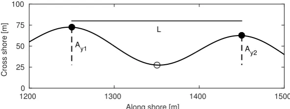
Fig. 8. A single crescent from the crescentic bar with lengthL and horizontal am-plitude ¯Ay = 0.5×(Ay1+Ay2)/2. The horn of the crescent is labelled with filled
circles, whereas the bay is labelled with an open circle.
4.2 Amplitude evolution 396
Due to the lack of observational data of the vertical amplitude of crescentic
397
bars, a straight comparison of the amplitude of the predicted dominant
length-398
scales with field observation is not possible. However, in Van Enckevort et al. 399
(2004), the horizontal amplitude ( ¯Ay) of the crescentic bar at Duck is recorded. 400
This amplitude was calculated as half the average cross-shore distance between
401
the bay and the two horns (Figure 8). We hypothesize that the vertical
am-402
plitudes of crescentic bars is proportional to ¯Ay. In figure 9, the predicted 403
amplitude of the dominant lengthscale (solid black curve) is compared with
404
the observed ¯Ay (dash-dotted blue curve). In the full model evolution, ampli-405
tude growth and equilibration after storm 1 is consistent with that observed.
406
After storm 3 the model produces more rapid growth to a higher amplitude
407
than that observed, but, nonetheless, qualitatively similar behaviour. Again,
408
the effect of the higher harmonic interactions may be observed by
compar-409
ing figure 9 (b) and (c). The differences are small, but remember that the
410
simulated amplitudes are those of the dominant lengthscale, and these are in
411
general over predicted by the equilibration model. A substantial difference
be-412
tween the observation and simulation is found after storm 2. In a short period
413
after storm 2, the observed amplitude recovers to the amplitude before the
414
storm, whereas very limited amplitude development is observed in our model
415
result. This, as also noted by Tiessen et al. (2010), points to the persistence
416
of bed-forms through the second storm. This will be further discussed in§5.2.
240 250 260 270 280 290
A
0 0.5 1
1.5(a) linear evolution
¯Ay
[m
]
0 20 40 60
240 250 260 270 280 290
A
0 0.5 1
1.5(b) equilibration
¯Ay
[m
]
0 20 40 60
Time [d]
240 250 260 270 280 290
A
0 0.5 1
1.5(c) full model
¯Ay
[m
]
[image:18.595.91.502.75.389.2]0 20 40 60
Fig. 9. Comparison between the observed and predicted dominant amplitudes, for three simulations: (a) linear evolution; (b) equilibration; (c) full model. The solid dark curve describes the amplitude of dominant lengthscale, whereas the dash-dot-ted blue curve refers to the observed longshore averaged horizontal amplitude ( ¯Ay).
5 Discussion
418
5.1 Importance of nonlinear effects 419
The most striking nonlinear effect on our simulation results is the higher
420
harmonic interaction. A quantitative comparison between the observed and
421
predicted lengthscales (Table 2) shows that the inclusion of higher harmonic
422
interaction reduced the absolute and relative error of predicted and observed
423
dominant length scale. The improvement in correspondence with the inclusion
424
of higher harmonic interaction is also apparent in Fig. 10 where the predicted
425
dominant lengthscale is compared to the observed lengthscale at the moments
426
when observations could be made. The incorporation of the equilibration term
427
is necessary.
Absolute error [m] Relative error [-]
Linear evolution 190 0.54
Equilibration 168 0.49
[image:19.595.148.431.74.155.2]Full model 108 0.31
Table 2
The error between predicted and observed dominant length scale of the different scenarios. Note that the comparison is taken at the moments when observation could be made, and both the absolute and relative error are averaged values.
λ
simulated [m]
0 200 400 600 800 1000
λobserved
[m]
0 200 400 600 800
1000 (a) linear evolution
λ
simulated [m]
0 200 400 600 800 1000
0 200 400 600 800
1000 (b) equilibration
λ
simulated [m]
0 200 400 600 800 1000
0 200 400 600 800
1000 (c) full model
2 10 35
Fig. 10. Comparison between the observed and predicted dominant lengthscales, for three simulated : (a) linear evolution; (b) equilibration; (c) full model. The area between the dashed lines corresponds to relative error < 0.3. The contour line denotes the density of data points, with red color for high density and blue color for low density, see color bar. The unit of color bar is ’number of observations (comparison) per unit area.’
5.2 The persistence of bed pattern after storms 429
In the model we have assumed that all pre-existing bed-forms have been
eradi-430
cated after each storm, and the development of all lengthscales starts from the
431
sameAmin. This assumption is based on the notion that each storm is powerful 432
enough and of long enough duration for an alongshore constant sandbar to be
433
formed. However, field observation shows that some crescentic bed patterns
434
can survive through a storm (Van Enckevort et al., 2004). After second storm
435
(Fig. 6), the field observed dominant length scales stay close to the length
436
scale before the storm, which are distinctly different to our model findings. As
437
previously postulated inTiessen et al.(2010), this might be due to the
persis-438
tence of crescentic bed-forms throughout a comparatively less powerful storm.
439
Moreover, apart from one observation at ∼ 700m (see Fig. 6) the observed
440
lengthscales right after the third storm stay in a narrow band close to the
441
dominant wavelength after the second storm. This is distinctly different from
442
the fluctuation of lengthscales observed after the first storm, and consistent
[image:19.595.101.490.218.380.2]with the aforementioned persistence of bedforms through the second storm.
444
To investigate this effect, we introduce a so-called persistence ratio (µ) of pre-existing bed patterns after a storm,
µ= Ak,t+s −Amin
Ak,t−
s −Amin
,
where t−s (t+
s) refers to the time immediately before (after) the storm. The
445
value of µ therefore ranges from 0 to 1, where µ = 0 (1) means that all
pre-446
existing bed-forms have been eradicated (preserved), so the initial amplitude
447
after storm Ak,ts+ = Amin(Ak,ts−). Previously (Fig. 6) µ = 0 is used for all
448
storms. Here we relate the value of µ to storm strength which is represented
449
by the maximum wave height of each storm. From this perspective, storm 2
450
and 3 are of similar strength, whereas storm 1 is more powerful, see Fig. 2.
451
We thus assume µ = 0 after the first, and investigate the effect of varying
452
the (same) value of µ after second and third storms for the full model (7). In
453
Fig. 11 (black dashed line) we see the effect of this variation inµ. By allowing
454
more bed amplitude to be preserved we observe a reduction in relative error of
455
lengthscale asµincreases from 0 (its value in Fig. 6), and thereafter a modest
456
increase. In fact, there is a max. error for µ= 0. Further research is required
457
to clarify the mechanism lying beneathµ. The sensitivity of model behaviour
458
onµ is further discussed in§ 5.4.
459
5.3 Energy transferred to higher harmonics 460
The energy transferred fromλ to λ2 is characterised by a factor α(see §3). As
461
mentioned in§3, the value of α in this study was chosen based on the rate of
462
energy transfer observed byTiessen et al.(2011). A high value ofαindicates a
463
rapid transfer of energy to λ2 and hence probably leads to an earlier post-storm
464
dominance of short wavelength. It is apparent (see Fig. 11 for µ= 0) that the
465
value used in Fig. 6 (following Tiessen et al., 2011) gives something close to
466
the minimum relative error for the full model.
467
5.4 Model sensitivity to µ and α
468
The full sensitivity of the full model behaviour toµand αis shown in Fig. 11,
469
with 0.2≤α≤0.8 and 0≤µ≤1 (note that we still assume thatµ= 0 for the
470
first, larger storm). The relative error of the predicted dominant lengthscales
471
and observed lengthscales is smaller for non-zero µ. This suggests that part
472
of pre-existing bed pattern (and therefore lengthscale(s)) persists after second
473
and third storms, and, by implication, that the second and third storm are not
α [-]
0.2 0.4 0.6 0.8
µ
[-]
0 0.2 0.4 0.6 0.8 1
full model
[image:21.595.193.391.70.285.2]0.2 0.3 0.4
Fig. 11. sensitivity of full model behaviour on persistence ratioµof pre-existing bed patterns and energy transfer factor α. The vertical black dashed line refers to the choice of α = 0.3 in section 4. Colours indicate the relative error of the predicted dominant lengthscales and observed lengthscales, with blue for low relative error and red for high relative error.
strong enough to erase all the existing bed forms. There is a region of broadly
475
minimum error for about 0.2 ≤ µ ≤ 1 and 0.3 ≤ α ≤ 0.6. The conclusion
476
appears to be that a higher µ after storm 2 and 3 leads to slightly better
477
correspondence between prediction and observation.
478
The minimum error is actually achieved (Fig. 11) for α= 0.41 and µ= 0.78,
479
resulting in a relative error of 0.24 (as compared to 0.31 for µ = 0, α = 0.3,
480
see Table 2). Using these values we re-run the model for the full duration,
481
and results are shown in Fig. 12. Additionally, we see results of the predicted
482
dominant amplitude plotted against that observed. The predicted dominant
483
amplitude now shows better correspondence with observation after the second
484
storm, but poorer correspondence after the third storm. This and Fig. 10
485
suggest that these two storms correspond to different µvalues.
486
6 Conclusions
487
In this study, we hypothesize that the dominant mechanisms for evolution of
488
crescentic bar systems in nature are linear growth allied to equilibration
(self-489
limitation) and higher harmonic generation by self-interaction. These
mecha-490
nisms have been implemented into a model that would result from a weakly
491
nonlinear perturbation analysis, but in which the coefficients of the
nonlin-492
ear terms (in particular, that governing higher harmonic interactions) are set
240 250 260 270 280 290
λ
[m]
200 400 600 800 1000
full model
0.1 0.4 0.7 1
Time [d]
240 250 260 270 280 290
A
0 0.5 1 1.5
¯Ay
[m
]
[image:22.595.99.483.77.398.2]0 20 40 60
Fig. 12. Amplitude (top, figure explanation is as Fig. 6) and dominant amplitude (bottom, figure explanation similar as Fig. 9) development for the full model with
α= 0.41 and µ= 0.78.
based on observations. This model is then used to investigate the bathymetric
494
evolution of a crescentic-barred beach at Duck (North Carolina, USA). The
495
model was used to reproduce a 2-month period, over which field observations
496
were analysed by Van Enckevort et al. (2004). Results show that nonlinear
497
effects of equilibration and higher harmonic interaction lead to significantly
498
improved reproduction of long-term evolution of a crescentic bar system in
499
terms of observed lengthscales.
500
In between storms when crescentic bars develop, their initial development
501
corresponds well with the results from a basic linear stability analysis. The
502
addition of a self-limitation term (Drazin and Reid, 1981) extends the
predic-503
tive range of the linear stability model to the entire post-storm period. The
504
inclusion of the term describing generation of higher-harmonics (as suggested
505
by Tiessen et al., 2011) leads to a significant improvement in prediction of
506
observed lengthscales. With these extra effects, an approach based on linear
507
stability analysis can describe the observed change from immediately
post-508
storm large lengthscales to the subsequent shorter lengthscales, related to
509
calmer conditions in between storm events, and the subsequent stabilisation
of the bed.
511
Note that the present approach is a significantly larger undertaking than that
512
of just determining a single fastest growing mode (F GM), i.e. corresponding to
513
a singlekat one time, as done byTiessen et al.(2010). Here we must determine
514
a whole, unique growth rate curve at each time. Nonetheless, the present
ap-515
proach is still significantly less demanding in terms of computational time than
516
the simulations typically required to describe the development of the whole sea
517
bed over this area (this is generally done using a fully nonlinear model, and
ei-518
ther 2DH or 3D). An additional advantage of the currently proposed method is
519
the significantly reduced need for beach-specific parametrisation, because
de-520
tailed, spatially-variable planform-bathymetric data is not required. Similarly,
521
only relatively idealised and schematised conditions regarding wave climate
522
and tidal elevation are needed for a linear stability approach.
523
Whilst these findings represent an improvement on a linear stability model
524
(Tiessen et al., 2010), several effects are not yet included or fully understood.
525
For instance, the occurrence of a storm-related eradication of the
crescen-526
tic bed-forms needs to be further investigated. The current research suggests
527
that certain storms might not be strong enough to cause a wipe-out of
along-528
shore bedforms. Additionally, the energy transferred in the higher harmonic
529
interaction is not yet quantified. More work is needed on developing a
system-530
atic approach to deriving the amplitude equations. Doing this would allow a
531
more complete description of long-term crescentic development (as opposed to
532
just lengthscale and amplitude). Note also that in our approach we consider
533
discrete wavelengths as opposed to the continuum of wavelengths that are
de-534
scribed by a Ginsburg-Landau equation (Schielen et al., 1993). Finally, note
535
that for some forcing conditions there is likely to be more than one physically
536
relevant growth rate curve (see Fig. 3).
537
Acknowledgements
538
The support of the UK Engineering and Physical Sciences Research Council
539
(EPSRC) under the MORPHINE project (grant EP/N007379/1) and of the
540
University of Nottingham is gratefully acknowledged.
541
References
542
Calvete, D., N. Dodd, A. Falqu´es, and S. M. Van Leeuwen, Morphological
543
development of rip channel systems: normal and near normal wave incidence,
544
J. Geophys. Res., 110(C10), C10,007, doi:10.1029/2004JC002,803, 2005.
Calvete, D., G. Coco, A. Falqu´es, and N. Dodd, (un)predictability in rip
chan-546
nel systems, Geophys. Res. Lett.,34(L05605), doi:10.1029/2006GL028,162,
547
2007.
548
Castelle, B., and B. G. Ruessink, Modeling formation and subsequent
nonlin-549
ear evolution of rip channels: Timevarying versus timeinvariant wave forcing,
550
J. Geophys. Res., 116(doi:10.1029/2011JF001997), F04,008, 2011.
551
Church, J. C., and E. B. Thornton, Effects of breaking of the longshore current,
552
Coastal Eng., 20, 1–28, 1993.
553
Damgaard, J. S., N. Dodd, L. J. Hall, and T. J. Chesher, Morphodynamic
554
modelling of rip channel growth, Coastal Eng.,45, 199–221, 2002.
555
Deigaard, R., N. Drønen, J. Fredsøe, J. H. Jensen, and M. P. Jørgensen, A
556
morphological stability analysis for a long straight barred beach, Coastal 557
Eng.,36(3), 171–195, 1999.
558
Dodd, N., P. Blondeaux, D. Calvete, H. E. de Swart, A. Falques, S. J. Hulscher,
559
G. Rozynski, and G. Vittori, Understanding coastal morphodynamics using
560
stability methods, Journal of coastal research, 19(4), 849–865, 2003.
561
Drazin, P. G., and W. H. Reid, Hydrodynamic Stability, 527 pp., Cambridge
562
Univ. Press, New York, 1981.
563
Falqu´es, A., G. Coco, and D. A. Huntley, A mechanism for the generation of
564
wave driven rhythmic patterns in the surf zone,J. Geophys. Res.,105(C10),
565
24,071–24,087, 2000.
566
Feddersen, F., R. T. Guza, and S. Elgar, Velocity moments in alongshore
bot-567
tom stress parameterizations, J. Geophys. Res., 105(C4), 8673–8686, 2000.
568
Garnier, R., D. Calvete, A. Falqu´es, and N. Dodd, Modelling the formation and
569
the long-term behaviour of rip channel systems from the deformation of a
570
longshore bar, J. Geophys. Res., 113, C07,053, doi:10.1029/2007JC004,632,
571
2008.
572
Hanley, M., S. Hogart, D. Simmonds, A. Bichot, M. Colangelo, F. Bozzeda,
573
H. Heurtefeux, B. Ondiviela, R. Ostrowski, M. Recio, R. Trude,
574
E. Zawadzka-Kahlau, and R. Thompson, Shifting sands? coastal
protec-575
tion by sand banks, beaches and dunes, Coastal Engineering, 87(0), 136 –
576
146, 2014.
577
Knaapen, M. A. F., and S. J. M. H. Hulscher, Use of a genetic algorithm to
578
improve predictions of alternate bar dynamics, Water Resources Research,
579
39(9), 1231, 2001.
580
Ribas, F., A. Falqu´es, H. E. de Swart, N. Dodd, R. Garnier, and D.
Cal-581
vete, Understanding coastal morphodynamic patterns from depth-averaged
582
sediment concentration, Rev. Geophys., 53(2), 362–410, 2015a.
583
Ribas, F., A. Falqus, H. E. deSwart, N. Dodd, R. Garnier, and D. Calvete,
584
Understanding coastal morphodynamic patterns from depth-averaged
sedi-585
ment concentration, Reviews of Geophysics,53(2), 362–410, 2015b.
586
Schielen, R., A. Doelman, and H. de Swart, On the dynamics of free bars in
587
straight channels, J. Fluid Mech., 252, 325–356, 1993.
588
Smit, M. W. J., A. J. H. M. Reniers, and M. J. F. Stive, Role of morphological
589
variability in the evolution of nearshore sandbars, Coastal Eng., 69, 19–28,
2012.
591
Soulsby, R. L.,Dynamics of Marine Sands, 249 pp., Thomas Telford, London,
592
1997.
593
Tiessen, M. C. H., S. M. van Leeuwen, D. Calvete, and N. Dodd, A
594
field test of a linear stability model for crescentic bars, Coastal Eng.,
595
57(doi:10.1016/2009.09.002), 41–51, 2010.
596
Tiessen, M. C. H., N. Dodd, and R. Garnier, Development of crescentic
597
bars for a periodically perturbed initial bathymetry, J. Geophys. Res.,
598
116(doi:10.1029/2011JF002069), F04,016, 2011.
599
Van Enckevort, I. M. J., B. G. Ruessink, G. Coco, K. Suzukui, I. L. Turner,
600
N. G. Plant, and R. A. Holman, Observations of nearshore crescentic
sand-601
bars, J. Geophys. Res., 109(C06028), 2004.
602
Van Leeuwen, S. M., N. Dodd, D. Calvete, and A. Falqu´es, Physics of nearshore
603
bed pattern formation under regular or random waves, J. Geophys. Res.,
604
111(F01023), 2006.