ORIGINAL ARTICLE
Self-Employment in an Equilibrium Model of the
Labor Market
Jake Bradley
Correspondence:jb683@cam.ac.uk
Faculty of Economics, University of Cambridge, Sidgwick Ave, CB3 9DD Cambridge, UK
Full list of author information is available at the end of the article
Abstract
Self-employed workers account for between 8% and 30% of participants in the labor markets of OECD countries,Blanchflower(2004). This paper develops and estimates a general equilibrium model of the labor market that accounts for this sizable proportion. The model incorporates self-employed workers, some of whom hire paid employees in the market. Employment rates and earnings distributions are determined endogenously and are estimated to match their empirical counterparts. The model is estimated using the British Household Panel Survey (BHPS). The model is able to estimate nonpecuniary amenities associated with employment in different labor market states, accounting for both different employment dynamics within state and the misreporting of earnings by
self-employed workers. Structural parameter estimates are then used to assess the impact of an increase in the generosity of unemployment benefits on the
aggregate employment rate. Findings suggest that modeling the self-employed, some of whom hire paid employees implies that small increases in unemployment benefits leads to an expansion in aggregate employment.
Keywords: Self-employment; job search; firm growth
JEL Classification: J21; J24; J28; J64
1 Introduction
The proportion of total employment made up by the self-employed in the U.K. rose steadily over the period 2000-2004. The number of self-employed increased by 8.9% compared with an increase of 0.1% of paid employees. This growth was across gender, region, and industry, Lindsay and Macauley (2004). Over this pe-riod the average self-employment rate was at 11.5% of total employment and this large proportion is not unique to the United Kingdom: across all OECD countries this proportion varied from 8-30%,Blanchflower(2004). Overall employment, wage determination and dynamics across the two sectors are clearly intrinsically linked, especially when one also considers that in the U.K. one third of all the self-employed
hire at least one paid employee, Moralee (1998). Considering the size and impor-tance of self-employment, literature that incorporates it into a model of the labor market is relatively sparse.
This paper develops a search-theoretic general equilibrium model of the la-bor market that incorporates self-employed individuals. The self-employed en-trepreneurs are treated in a Schumpeterian way, as a source of innovation, Schum-peter(1934, reprinted in 1962)[1]. It is distinct from other labor market models of
[1]For a comprehensive discussion of the history of economic thought regarding entrepreneurship
self-employment in that after innovation the self-employed agent can work on their own, as an own-account worker, or begin hiring workers from a labor market with search frictions. The importance of incorporating the self-employed into an equilib-rium model of the labor market is seen by looking at simulations of labor market policy. Conventional wisdom would suggest a rise in unemployment benefits would have an adverse effect on aggregate unemployment - workers require better job of-fers or betterideas to exit unemployment for paid or self-employment respectively. Introducing the self-employed as a source of job creation introduces a counterweight to this straightforward mechanism. If only sufficiently good ideas create employment opportunities, making the self-employed more fastidious about which ideas to act on could create employment opportunities for other agents. This paper finds that for small increases in the generosity of unemployment benefits aggregate employ-ment increases. This is used as an illustrative example to show the importance of considering the self-employed when implementing active labor market policy.
In the model there are two types of agents, large private sector firms who vary in their productivity and ex ante homogeneous workers who are exposed to innovative ideas which arrive at an exogenous Poisson rate that is dependent on their labor market status. When an agent gets an idea its quality is drawn from a known distribution and the agent decides whether to act on it. If they choose to start a business, then depending on the quality of the draw they may commence attempting to hire workers as paid employees. Thus paid employees are either hired by large firms or self-employed recruiters. All workers are finitely lived and when in paid employment are exposed to an exogenous probability that they lose their job; all wage offers and job arrival rates to paid employment are determined endogenously. This rich setting allows for a multitude of avenues in which the two sectors are interlinked.
The model is structurally estimated using the British Household Panel Survey (BHPS). The identification strategy allows primitive productivity distributions and hiring behavior of both types of firm to be uncovered. The distribution of productiv-ity amongst large firms is uncovered, as inBontemps et al(2000) by an inversion of the wage offer distribution; the productivity amongst the self-employed is obtained directly from their earnings; and hiring behavior is estimated in order to match the distribution of firm size amongst large privately owned companies and small firms owned by self-employed recruiters. Estimates suggest that the productivities of the two types of firms are very similar, however self-employed owned firms are responsible for a much smaller share of employment because they face much greater frictions in hiring paid employees. It is necessary to uncover output and hiring through the guise of an equilibrium model as there exist large limitations of data on the self-employed. Data are specifically limited in information regarding the re-cruiting self-employed. The BHPS is useful as it distinguishes the self-employed between those who hire paid employees and those who do not. However, it does not identify the paid employees who are hired by recruiting self-employed nor does it provide information on output. Therefore in order to infer rates of hiring and pro-duction the paper leans heavily on a model that provides a great deal of structure to the data.
types of self-employment discussed.Kumar and Schuetze(2007) develop a model of the labor market that incorporates self-employment and assess the effect of changes to unemployment insurance and the minimum wage on labor market equilibrium. Self-employed hire paid employees as in this paper, but unlike this model there is no wage dispersion within sector nor are there any movements across sectors. Thus
they restrict a direct interaction between the two sectors. Narita(2014) and Mar-golis et al (2014) allow for wage dispersion within sector and structurally estimate the parameters of their models using data from Brazil and Malaysia, respectively. However, unlikeKumar and Schuetze(2007) and this paper, the self-employed are
restricted to being own account workers (they are restricted from hiring). Also, al-though they allow for more mobility than Kumar and Schuetze (2007), they still omit any direct transitions between paid and self-employment.
Although not all concern themselves with self-employment, perhaps the most similar papers methodologically are Meghir et al(2015),Bradley et al (2015) and
Mill´an(2012). All introduce another sector into an equilibrium labor market setting allowing for a great deal of mobility between and across sectors, be it an informal, public or self-employed sector. Decisions made by workers depend not only on the wage they are offered but future prospects associated with the sector.Mill´an(2012)
suggests that self-employment is used as a route out of unemployment. This paper does not consider this hypothesis, but workers may be encouraged to become self-employed as they face the opportunity of starting a business which can grow. Only
Kumar and Schuetze (2007) and this paper entertain the idea of the self-employed as employers and only this paper distinguishes between the self-employed as own
account workers and recruiters.
The consensus in the empirical literature is that there exists a substantial paid employment premium over being self-employed. Hamilton (2000) finds that tak-ing into account within sector earntak-ings growth and without disttak-inguishtak-ing between
own account self-employed and recruiters, there is a 35% differential between me-dian earnings of a self-employed individual and a paid employee with ten years of experience in the U.S. To rationalize workers’ career choices, “results suggest that the nonpecuniary benefits of self-employment are substantial”. Critiquing the shortcom-ings of the existing literatureHamilton(2000) goes on to say “results presented here
are of a reduced form [...] structural estimates of the compensating wage differential, for example, would require [...] the probability of observing particular employment and earnings sequences”. To my knowledge, this is the first paper that attempts to structurally estimate the nonpecuniary benefits of self-employment while taking
into account different employment options, including starting and growing one’s own business. A priori it is not clear which sector has the preferable employment and earnings profile. On the one hand, those in paid employment are better exposed to other jobs in paid employment and can climb the job ladder thusly. However, the self-employed are far more likely to become recruiters. If their firm successfully
grows so will their earnings. Consistent with the empirical literature, this paper too finds a large positive amenity associated with self-employment.
The rest of the paper is structured as follows. Section 2 presents and solves the equilibrium model. Section 3presents the data, which corrects the earnings of the
the moments used for identification. Section4outlines the estimation protocol, the results and the fit of the model. Section5runs counterfactual policy simulations to
asses the effects of increasing unemployment benefit on aggregate employment and finally, Section 6concludes.
2 The Model
2.1 The Environment
Time is continuous, and at any point there exists a unit mass ofex-ante
homoge-neous workers and a massN of private sector firms who are heterogeneous in their level of productivity. Workers and firms are risk-neutral and discount the future at
a rater >0. Workers can be in one of three broad states: unemployment, paid em-ployment or self-emem-ployment. They leave the labor market at an exogenous Poisson rateµwhich is independent of their labor market state; they are replaced with new agents who are born into unemployment. Firms are infinitely lived[2].
Paid employment comes from two sources, large private sector firms and
self-employed individuals. Job offers arrive to unself-employed agents from firms at a rateλ0
and paid employees in large firms at a rateλ1=κλ0.κis the relative search intensity
of an employed worker compared to an unemployed one. Wages are drawn from a known distributionF(·). Job offers can also arrive from self-employed recruiters at a rateλs
0to the unemployed. For tractability, it is assumed that the recruiters direct
all their search intensity to the unemployed, attempts will be made to justify said
assumption in Section 3. These wages are drawn from a known distribution Fs(·).
All job offer arrival rates and wage offer distributions are endogenous objects. A
match is destroyed at a Poisson rateδ. Both firm and worker continue to exist, but, the worker is reallocated to unemployment. If the worker exits the labor market, at a rate µ, the firm will continue to exist, but with one less worker. Agents are also exposed to the possibility of having an innovative idea. The rate agents get ideas follows a Poisson process which is dependent on one’s labor market state.
Ideas arrive to unemployed agents at a rateη0and to paid employees in large firms
at a rate η1. The quality (productivity) of the idea is drawn from an exogenous
distribution Γ(·). Depending on the draw this will allow workers to cross the market from unemployment or paid employment and become self-employed. The reservation
productivity of paid employees will depend on their current wage.
Self-employment spells begin as an agent working on his own producing output according to the draw from Γ(·). There is a search friction in the matching process: hiring workers takes time. One can think of this as time required for vetting,
pre-liminary training etc. So, as will transpire, some of the self-employed will wish to
hire but are time restricted and therefore hire at a suboptimal rate.
It is assumed that the self-employed hire at a Poisson rateh`, wherehis exogenous and constant for all firms (independent of size and productivity) and`is the size of the firm, and can take any positive integer value. Thus, by construction, the growth
[2]Firms are assumed to be infinitely lived to keep features of theBontemps et al(2000) model.
of a firm adheres to Gibrat’s law[3]. The rate of total hiring is proportional to the firm size as the hiring process requires a certain amount of work. Larger firms can share this workload over a greater number of workers and hence the rate of hiring
increases proportionally with the size. In a way akin toColes and Mortensen(2011), the size of the firm `will follow an endogenously determined Markov process.
Finally, the model is derived in a steady-state. The stocks of agents in each of the three states are constant over time as are the distributions of firm size, productivity amongst the self-employed and the distribution of wages amongst the paid
employ-ees. To solve the model one needs to: (i) derive the value functions of the three states; (ii) derive reservation levels for which workers change states; (iii) calculate the size of each state and derive the ergodic distributions of wages and productivity
within states; (iv) derive the profit maximizing wage policy of large private sector firms.
2.2 Value Functions
Workers can be in one of five states: paid employment in a large firm;
unemploy-ment; paid employment, employed by a employed recruiter; own account self-employment (working alone); and recruiting self-self-employment (hiring paid employ-ees). In all states workers are maximizing their lifetime income discounted at a rate
r. The following subsections derive the lifetime values for each state.
2.2.1 Paid Employees
A paid employee working for a large firm has two sources of revenue flow from em-ployment, a basic wage and a nonpecuniary amenity, whichex-ante can be positive
or negative; it is measured relative to being a self-employed worker. As well as the revenue flow of income and amenity, the value function of a paid employee has the option value of transiting into other states, namely the option value of
unemploy-ment, higher value paid employment (employed by firm or a self-employed agent) and self-employment. At any point there is a possibility that the agent exits the labor force. All future revenue flows are discounted at a rate r.
The value function for a paid employee earning a wagewin a large firm is given by[4]
(r+µ)W(w) =w+a+δ[U−W(w)] +λ1EFmax [W(x)−W(w),0]
+η1EΓmax [S(z)−W(w),0]. (1)
An individual exits to unemployment at a rateδwhen the match dissolves. They receive other job offers from firms at a rate λ1 and they have innovative ideas at a
rateη1. After an idea a private sector employee either stays employed or becomes
self-employed which gives value S(z), wherez is the productivity draw. If the idea is sufficiently good, they leave to self-employment, and initially, work individually,
[3]The empirical evidence on Gibrat’s law in relation to firm growth is mixed. For a summary of
the literature seeSantarelli et al(2006).
[4]
EFmax [W(x)−W(w),0] =
R
max [W(x)−W(w),0]dF(x) and EΓmax [S(z)−W(w),0] =
R
as an own account worker. The value for unemployment is given by equation (2), where bis the flow value of unemployment, relative to self-employment.
(r+µ)U =b+λ0EFmax [W(x)−U,0] +η0EΓmax [S(z)−U,0]
+λs0EFsmax [Ws(x)−U,0] (2)
If a paid employee is hired by a self-employed agent, they face very different opportunities than if they are employed by a large firm. The validity of these
as-sumptions will be addressed when looking at the data in Section 3. Firstly, as the firm is relatively small it is assumed that the actions of the workers are observable
to the self-employed recruiter. Thus the worker spends no time searching for other jobs or thinking about innovative ideas. Therefore in addition to exiting the labor market, the only other potential transition facing the employee is to unemployment.
This occurs more frequently than in paid employment in a large private sector firm because not only does the worker contend with the possibility the match is
de-stroyed, at rate δ, but the recruiter employing him can also exit the labor market, at a rate µ. Like a paid employee in a large firm, the amenity associated with paid employment in a self-employed owned firm is given by the flow benefita. The value function for a paid employee earningwworking for a self-employed recruiter is:
(r+µ)Ws(w) =w+a+ (µ+δ) [U−Ws(w)] (3)
2.2.2 The Self-Employed
All self-employed agents start their self-employment spell as an own account worker. That is they employ only themselves. If an agent aims to recruit workers they will
arrive at a rate h`, where `is the integer number of employees they already have. Workers will quit the firm at a rate (µ+δ), exiting to either unemployment or out of the labor force. Thus the number of workers a recruiter employs will follow a
Markov process. The only search friction that exists for a recruiter is that hiring is a time consuming process. For a firm with an integer number of employees`, it takes an estimated time 1/h`to hire a worker. Unlike theBurdett and Mortensen(1998)
model, a higher wage neither increases the rate of recruitment nor retention. For ease of exposition it is assumed that the self-employed never exit self-employment
for unemployment.
To begin with, attention is restricted to those self-employed whose interest it is to recruit workers. Then at the start of a self-employment spell an agent produces as
an own account worker, his output is equal to his productivity and at a ratehwill hire a worker. The value function for a newly self-employed agent of productivity
y who intends to recruit is given in equation (4), where R(y,1) is the value of a self-employed individual with productivityy and one employee.
If a self-employed agent does find a worker, he foregoes his own output in order to manage the newly created firm. However, the production per worker is nowp(y), wherep(y) is the productivity per worker of a self-employed owned firm of qualityy. Any worker employed produces output using the self-employed agent’s technology,
p(y), and receives an endogenously determined wage,w?(y, `). Some regularity
con-ditions are imposed onp(y), they are, thatp0(y)>0 for allyandp00(y)≥0 for ally. Intuitively one might expectp(y)> y, as the firm has management oversight, how-evera priori only the two regularity assumptions are assumed. The value function
for a recruiter is given by R(y, `), wherey is the productivity and` is the integer number of workers employed. The right hand side of equation (5) contains: the profit
flow, production net of wages; plus the probability of expanding employment by one employee multiplied by the option value of that occurrence; plus the equivalent for
losing one worker, either the worker returns to unemployment or leaves the labor
force entirely. Equation (5) is expressed for one worker and an arbitrary amount of workers`.
(r+µ)R(y,1) =p(y)−w?(y,1) +h[R(y,2)−R(y,1)] + (µ+δ) [R(y,0)−R(y,1)] ..
.
(r+µ)R(y, `) = (p(y)−w?(y, `))`+h`[R(y, `+ 1)−R(y, `)]
+ (µ+δ)`[R(y, `−1)−R(y, `)] (5)
The recruiter setsw?(y, `) to maximize his present discounted value. Since posting vacancies and hiring are costless (other than time) there is no incentive to pay higher
wages to attract workers. In addition, the recruiter does not need to pay a higher wage to retain his workers, as there is no retention motive. He observes them not
looking for other jobs or innovative ideas. He cannot, however, pay them nothing;
he must pay a sufficiently high wage such that some workers want to be employed. The recruiter exclusively hires from the pool of unemployed therefore the wage paid
makes workers indifferent between remaining unemployed and accepting an offer.
That isWs(w?(y, `))≥U; a worker must be at least as well off in paid employment than they are in unemployment. The recruiter’s problem is:
max
w?(y,`)R(y, `) subject to W
s(w?(y, `))≥U (6)
Since the value of recruitment decreases with the wage rate, the optimal wage is
independent of y and` and solves the equalityWs(w?) =U. An explicit solution will be given for w? in the next section.
Further, it is assumed that if a recruiter has just one employee, if that employee
leaves the firm, the firm and the self-employed individual cease to exist (retires)
this, the difference equations specified in equation (5) are linear in`. With this in mind, it is trivial to see that
R(y, `) =`R(y,1). (7) Thus equation (5) simplifies to
R(y,1) = p(y)−w
?
r+ 2µ+δ−h. (8)
Substituting equation (5) into equation (4), one can obtain the recursive solution for the value of becoming self-employed and intending to recruit with productivity
y
SR(y) =
y(r+ 2µ+δ) +h(p(y)−y))−hw?
(r+ 2µ+δ−h)(r+µ+h) . (9)
However, it is not clear whether it is in the interest of the self-employed to hire any paid employees. They have to forfeit their own production and increase their chance of going under. Looking at equation (9), as the wage they pay their employees increases, the value of self-employment with the intention to recruit decreases. The value function of a self-employed individual of productivity y to remain an own account worker will be just their output, which they get indefinitely (unless they exit the labor market).
(r+µ)SO(y) =y (10)
For an individual not to set about recruiting, the option value of having one worker must be negative. A self-employed individual with productivity y will aim to recruit workers ifSR(y)≥SO(y). Given certain regularity conditions, to follow,
there exists a threshold productivity level ψ1, above which self-employed agents
intend to recruit.
So the value function for a newly self-employed agent is given by equation (11). Fory∈[ψ0, ψ1) an agent will make no attempt at hiring and their value function is
simply the present discounted value of constant production of amounty. Ify≥ψ1,
they will initially be an own account worker, but will hire someone with Poisson rate
hand produce an amount p(y), paying w? to their employee. Thus the expression is increasing inhand inp(y) and decreasing inw?. It is also decreasing inr,µand
δ, the discount rate and the Poisson rates of agents leaving the labor market and job destruction, respectively.
S(y) =
( y
r+µ ify < ψ1 y(r+2µ+δ)+h(p(y)−y))−hw?
(r+2µ+δ−h)(r+µ+h) ify≥ψ1
2.3 Reservation Strategies
A worker’s strategy can be characterized by a set of reservation values which de-pends on his current labor market state.
The wage a paid employee receives in a large firm that makes him indifferent be-tween becoming self-employed of productivityyand remaining in paid employment is defined as φ(y). Similarly the productivity a paid employee will require to enter self-employment isψ(w). These functions solve the equalities:
S(ψ(w)) =W(w) S(y) =W(φ(y)) (12) Using the above two equations:
S(y) =W(φ(y)) =S(ψ(φ(y))) (13) Thus,
y=ψ(φ(y)) (14) Hence, given monotonicity of the value functions, ψ and φ are reciprocals of one another. Similarly, the wage that makes an unemployed agent indifferent between continuing unemployment and being employed by a large firm is φ0and solves the
equality W(φ0) =U, and the productivity of an idea that makes an unemployed
agent indifferent between continuing unemployment and being self-employed at that productivity isψ0and solves the equality S(ψ0) =U. Clearly,ψ(φ0) =ψ0.
To find solutions for these reservation strategies, it is convenient to begin by simplifying the value functions for workers: Firstly, Ws(w) = Ws, as Fs(·) is a
degenerate distribution atw?. SinceWs=U, a worker never gets a positive option
value from being employed by a self-employed recruiter, therefore it drops out of the Bellman equations. Finally, in calculating the expectation, one can integrate by parts, where the overscore on the distribution represents the survival function, for example,F(·) = 1−F(·). Thus equations (1), (2) and (3) simplify to (15), (16) and (17), respectively.
(r+µ)W(w) =w+a+δ[U−W(w)] +λ1 Z
w
W0(x)F(x)
dx
+η1 Z
ψ(w)
S0(z)Γ(z)
dz (15)
(r+µ)U =b+λ0 Z
φ0
W0(x)F(x)dx+η0 Z
ψ0
S0(z)Γ(z)dz (16)
Ws= w
?+a
r+µ (17)
2.4 Steady State
The model is derived in a steady state. A steady state is defined as a constant share of agents in each labor market state, and the distributions of wages amongst the paid employees, the productivity amongst the self-employed and the distribution of employment size amongst recruiters are all stationary.
The steady state is defined by equations (18) through (21). The sum of all agents in the economy is equal to unity. The flow into unemployment equals the outflow. The flow out of self-employment (paid employment) below a productivityy(wagew) is equal to the flow into self-employment (paid employment) below a productivityy
(wagew). As well as this, the distribution of labor force size amongst self-employed recruiters that is dictated by a Markov process has reached its ergodic distribution. This last object is denoted as Σ(`); it is the measure of recruiters and those who intend to recruit hiring an integer` workers.
An agent can be in one of three broad states and the sum of agents is equal to unity: they can be unemployed, in paid employment (by a large firm or a self-employed recruiter) or in self-employment. One could also differentiate further, defining those self-employed, recruiting or with the intention to recruit and those who are own account workers.
Nu+ (Nef+N s
e) +Ns= 1 (18)
The flow out of unemployment, the left hand side of equation (19) is made up of
four flows. In the order they are expressed they are: those leaving to paid employ-ment in large firms; those leaving to be self-employed; those exiting the labor force; and those becoming employed by small self-employed recruiters. This last flow is equal tohNs
e+hΣ(0). The rate at which the self-employed hire is equal toh
mul-tiplied by the total number of agents engaged in hiring, that is all the employees (Nes) plus the recruiters who are yet to hire any workers (Σ(0)). The flow exclusively comes out of unemployment as anyone in paid employment (by large firms) would reject any offer. The flow into unemployment is comprised of all the new entrants into the labor market plus the paid employees whose employers have exited the
labor market. New entrants arrive at a rate that exceedsµ. Firms of size one have a double coincidence of exiting the labor market, as discussed earlier. They also leave the labor market if they lose their final worker.
Nu λ0+η0Γ(ψ0) +µ
+h(Nes+ Σ(0)) =µ+ (µ+δ)Σ(1) + (µ+δ)Nes+δNef (19) Equation (20) equalizes the flow in and out of self-employment below a produc-tivity level y. Γ(·) is the primitive distribution from which agents draw the pro-ductivity of their ideas from and Γs(·) is the distribution of productivity amongst
state to being out of the labor force. This exit rate increases once they start recruit-ing. Hence the equation is split either side of y =ψ1. If they have one employee
they will cease to exist if that one employee exits the labor force. The proportion of self-employed recruiters with exactly one employee is given by Σ(1)
NsΓs(ψ1).
Fory < ψ1:
NsΓs(y)µ=Nuη0[Γ(y)−Γ(ψ0)] +Nefη1 Z φ(y)
φ0
[Γ(y)−Γ(ψ(x))]dG(x) and fory≥ψ1:
NsΓs(y)µ+Ns(Γs(y)−Γs(ψ1))
(µ+δ)Σ(1)
NsΓs(ψ1)
=Nuη0[Γ(y)−Γ(ψ0)]
+Nefη1 Z φ(y)
φ0
[Γ(y)−Γ(ψ(x))]dG(x) (20)
For those in paid employment in large firms below a wageφ(y), agents exit paid employment to unemployment at a rateδ, they exit the labor force entirely at a rate
µ. They find higher paid jobs in large firms at a rate λ1F(φ(y)). Paid employees
can also exit to self-employment; they get an innovative idea at a rate η1 and will
act on it depending on their current wage and the quality of the draw they get from Γ(·). The inflow is entirely from unemployment.
NefG(φ(y))(µ+δ+λ1F(φ(y))) +Nefη1 Z y
ψ0
Γ(z)dG(φ(z))
=Nuλ0F(φ(y)) (21)
Equations (18), (19), (20) and (21) are solved simultaneously for the endogenous objects (Ns
e, Nu, NefG(φ(y)), NsΓs(y)). These coupled with the distribution Σ(`)
define the steady state allocation of agents. The solution for these objects is provided in AppendixA.2.
2.5 Private Sector Firms
Private sector firms are large and infinitely lived. The law of large numbers is em-ployed and they are modeled followingBontemps et al(2000). This paper considers the familiar equilibrium where firms post wages and commit to those wages for their lifetime. The higher the wage a firm posts, the larger the firm (fewer quits and more hires); this is at the cost of making less profit per worker. As pointed out
byColes(2001) this is not a dynamically consistent wage posting strategy without commitment on wages. To see this, imagine a firm has grown to its steady state size. Rather than posting its optimal wagew, it will be strictly better off to pay its workers’ reservation wage φ0. Over a period dt → 0 no workers will quit and the
firm will make strictly greater profits.Coles(2001) identifies a dynamically consis-tent equilibrium without relying on commitment. Interestingly, the wages posted by self-employed recruiters are a dynamically consistent strategy, without having
regarding dynamic consistency, the tractability of Bontemps et al (2000) makes it very well suited to modeling the behavior of large firms.
There exists a continuum of infinitely lived private sector firms of mass N who are profit maximizers and heterogeneous in their level of productivity, y, where
y ∼Γf(·). Each firm has the same exposure in the labor market and all receive a
mass of contacts at an exogenous Poisson rate hf. Unlike self-employed recruiters,
it is assumed that large private sector firms are in some way detached from the labor market and cannot target a specific subgroup of job seekers. Thus not every contact is associated with a hire. The steady state size of a firm posting a wage w
is therefore a function of the proportion of contacts it makes that accept the offer,
a(w), and the number who are in employment and quit ∆(w).
a(w) =λ0Nu+λ1N
f eG(w)
λ0Nu+λ1Ne
∆(w) =µ+δ+λ1F(w)
The size of a firm posting a wagew, is given by`f(w) and solves the flow balance
equation:
`f(w) ∆(w) =hfa(w) (22)
By setting a wagew, a firm of productivityy will be of size`f(w) and thus have
total profit given by:
max
w≥φ0
π(w;y) = (y−w)h
fa(w)
∆(w) (23)
The firm’s problem is solved by the first order condition:
y−w= a(w)∆(w)
a0(w)∆(w)−a(w)∆0(w) (24)
Thus if wages are increasing in productivity, then one can infer that F(w) = Γf(y(w)), where the relationshipy(w) is given by (24) and Γf(·) is the cumulative
distribution of productivity amongst large private sector firms. Thus the distribu-tion of wage offers in the private sector, F(w) can be retrieved if we know the distribution of productivity across firms.
To close the model, labor demand is fully endogenized. The total number of con-tacts from firms that workers receive is given by:
M =λ0Nu+λ1Nef
The total jobs offered by firms is the product of the mass of firms and the number
looking for a job while employed by a large firm, relative to being in unemployment,
λ1 = κλ0. The arrival rate of job offers from private sector firms to unemployed
agents is then given by:
λ0=
N hf Nu+κN
f e
(25)
2.6 Equilibrium Characterization
Given exogenous parameters r, a, b, µ, δ, η0, η1, h, p(y), κ,Γ(·),Γf(·), N, hf: an
equi-librium is characterized by the following conditions: (i) agents behave optimally
in their career decisions, solutions to φ0, ψ0, ψ1 and φ(y); (ii) the economy is in
steady-state, the inflow from a given state equals the outflow, solutions to Γs(·),
G(·), Nu, Nef, Nes, Ns and Σ(`); (iii) large private sector firms and self-employed
recruiters offer their workers’ wages optimally, w(p) and w? and (iv) when firms
behavior is aggregated the wage offer distribution F(·) and the offer arrival rates
λ0,λs0andλ1are determined. Attention is restricted to a specific class of equilibria
where self-employed individuals exist, some of whom recruit paid employees. To
guarantee this equilibrium, the exogenous parameter space needs to be constrained.
Assumption 1h∈(0, r+ 2µ+δ)
Assumption 2Eitherp0(y)≥0 andp00(y)>0 orp0(y)> r+2rµ++µδ−h andp00(y)≥0.
Proposition Given Assumptions 1 and 2, an equilibrium will exist with self-employed recruiters.
The intuition is as follows, these assumptions are needed for two reasons. Firstly, Assumption 1 guarantees the non negativity of the value function of a recruiter,
see (8). Given this, Assumption 2 guarantees that for a sufficiently good idea a self-employed agent will actively seek to hire workers.
Proof:For an individual to consider self-employment as a viable option it must
yield a positive value. A recruiter with one employee has value given by equation (8). Clearly, he must make positive profit per worker (p(y)> w?)
R(y,1) = p(y)−w
?
r+ 2µ+δ−h
The above is positive if Assumption 1 holds. Recruiters will exist if, for some y, the value of intending to recruit,SR(y), is greater than being an own-account
self-employed indefinitely, SO(y).SO(y) is a linear function of y and SR(y) is a linear
function ofp(y). Ifp0(y)≥0 andp00(y)>0, the first part of Assumption 2. Clearly, for sufficiently largey,SR(y)> SO(y) and given Assumption 1, recruiters will exist
in equilibrium.
Ifp(y) is linear and increasing iny, the second part of Assumption 2. Then both
SO(y) andSR(y) are linear and increasing iny. Thus for sufficienlty largey, recruiter
will exist ifSR0 (y)> S0O(y). This is the case, givenp0(y)> r+2rµ++µδ−h , contained in Assumption 2. Q.E.D.
Identification Result: A sufficient condition for the existence of recruiters is
For given p(y), r, δ and µ, one can guarantee the existence of recruiters (given Assumption 1 holds) if:
p0(y)> max
0<h<r+2µ+δ
r+ 2µ+δ−h
r+µ
p0(y)> r+ 2µ+δ r+µ
Class of Equilibrium: the equilibrium is restricted to one where self-employed
recruiters exist. Clearly, some self-employed will be own account workers. These
can fall into two categories either they are own account workers, but because of the
frictions present in the market, as yet, they have been unable to hire anyone. Or, they are own account workers with no intention to recruit. For the latter type of
agent to exist it is required that S0(y) > SR(y) for some y and because SR0 (y)>
S0O(y) for all y, this is equivalent toSO(ψ0)> SR(ψ0).
Since, one cannot restrict attention to either class as neither can be invalidated by
data any simulation of the model needs to repeatedly check in what equilibrium it is
in. One where, all self-employed intend to recruit or one where some self-employed intend to stay own account indefinitely.
3 Data
The model described is estimated using the British Household Panel Survey
(BHPS). It is identified using transition rates across labor market states, the
earn-ings of paid employees and self-employed workers and the distribution of firm size.
Exogenous parameters are estimated by simulated method of moments. The
prin-ciple of the estimation technique is to find values of the structural parameters that
minimize a function of the difference between a chosen set of moments from the
data and data simulated with these values of the structural parameters.
Of the exogenous parameters, the only one that is not estimated is the discount rate r. r is calibrated as equal to 0.0043, which is the monthly (continuous time) equivalent of a 5% annual rate. In order to estimate the distribution from which the
self-employed draw their level of productivity, a parametric assumption is made. It is assumed that Γ(·) follows a log-normal distribution with the mean and standard deviation of the associated normal given bymyandsyand the production function
of self-employed recruiters is specified as p(y) =βy. Thus, the rest of this section concerns itself with the estimation of the vector of exogenous parametersθ:
θ= h, η0, η1, µ, β, my, sy, a, b, κ,Γf(·), hf, N (26)
The role of the rest of the data section are twofold. Firstly, it aims to inform the
reader about the data that is used to estimate the model. Secondly, it attempts to
find empirical support for predictions of the model as well as assumptions made for
3.1 The Sample
The data used in the analysis are taken from the BHPS, a longitudinal dataset of British households. Data were first collected in 1991, but attention is restricted to five waves covering the period from 2004 to 2008. The sample comprises of prime-age (21-60) white male low-skilled workers. Low-skilled is defined as not having
obtained A-level qualifications. These are the highest qualifications available for students aged 18 in the UK, before they enter higher education. A worker is an individual who is never inactive in the period looked at: if out of work, they declare themselves to be actively seeking work. The hourly earnings distribution is adjusted
by treating the bottom and top 2.5% of the distribution as missing, hopefully ridding the sample of erroneously reported earnings.
Data are homogenized to include only low-skilled workers as agents are ex-ante
homogeneous so its important they are of similar skill in the data. Implicitly, it has been assumed that agents are exposed to employment opportunities at the same
rate within a labor market state. This seems less of an imposition on the data for low-skilled workers, as many high skilled professions exist where agents become self-employed more frequently. In addition, the type of self-employment more prevalent amongst high-skill workers, being made a partner of a firm for example, is less in
keeping with the arrival of an innovative idea, as modeled in this setup. Information on cross-sector differences in employment, hours worked and earnings are reported in Table 1. Following the methodology of Hurst et al (2014), using British con-sumption data, the earnings of the self-employed are adjusted to take into account any misreporting of earnings. This exercise is explained in detail in AppendixA.3.
The adjustment is relative to paid employment, one interpretation is therefore how much the self-employed under/over state their income relative to paid employees.
INSERT TABLE 1 HERE
There are a number of points worth noting from Table1. There is a non-negligible share of recruiters, consistent with the findings of Moralee (1998), with approxi-mately one third of self-employed agents hiring paid employees. The self-employed work longer hours than their paid employee counterparts and the recruiting
self-employed work significantly more still. There is a clear ordering in the second mo-ment of the earnings distribution across the three labor market states irrespective of whether one looks at the raw or the adjusted data. The ordering of the first moment is ambiguous however; the preferred specification that will be used in estimation
is the adjusted data. Looking at the large implied differences, the importance of correcting for the misreporting of earnings is evident. The ranking of the second moment of the earnings distribution is not targeted in the estimation, but will still be replicated by the theoretical model.
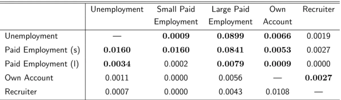
Table2 shows monthly worker turnover observed in the data. For the most part,
the cells of Table2are self-explanatory. The diagonal elements are all unobservable with the exception of workers changing jobs within paid employment. Although it is possible that a business goes bust and one instantly starts up a new one, this phenomenon is not possible to observe using the BHPS so transitions within specific
who declared their establishment to have fewer than 25 people working in it. Small and large firms are differentiated between because very few recruiters have 25 or more employees, see Table4. Therefore, the large firms provide a better indication of mobility for the paid employees hired by large private sector firms.
INSERT TABLE 2 HERE
The rates in bold are those that the model is capable of replicating, some of which the estimator will target, and those in plain text are ones that the model is unable
to generate. The model is unable to generate a number of classes of transitions. One is any transition into self-employment where the worker instantly becomes a recruiter. This is inconsistent with a labor market with search frictions, as one cannot hire individuals instantaneously. The second is a simplifying assumption made for tractability: once in self-employment an individual is allowed little labor
market mobility. Of the transitional moments omitted, the rate at which a recruiter transits to being an own account worker is the most glaring. In a given month there is a 1% chance of a recruiter losing its workforce and becoming an own account worker. This model is not able to generate this, in order to keep the result that a
recruiter’s value is proportional to the number of employees it has (equation (7)), which helps the tractability of the model. Also, while 1% seems large, in fact, from Table1just 4.6% of employed individuals are recruiters so this translates into very few transitions missed. Finally, as in models of wage posting, firm heterogeneity and on the job search like Bontemps et al (2000) , there is a one-to-one relation
between firm size and offered wage. In an identical way, this model can therefore not rationalize why a paid employee would take a wage cut and move to a smaller firm.
The parameter h is identified using the transition rate from own account employed to becoming a recruiter. Since the employee size distribution of self-employed recruiters is governed byµ, δ andh, this could be an alternative source of identification, conditional onµandδ. The firm size distribution amongst private sector employers is used to identifyhf, the volume of vacancies a single firm posts.
The self-employed are asked how many people they employ; the paid employees are
asked how many other people are in their place of work. These numbers are grouped into size bins and from these it is difficult to infer the size distribution of private sector firms. Therefore, purely for comparison, data on firm size from the Office of National Statistics (ONS) in the midpoint of the sample period is used.
The downside of comparing the size distributions in Tables 3 and 4 is that the size bins do not correspond to one another. The cumulative firm size distribution at employee sizes 9, 49, 99, 499 and 999 can be compared. Firms owned by the self-employed are typically smaller than firms at large, 86.1% of self-employed run firms have less than 10 employees, compared with 82.02% of all firms. Similarly,
96.69% of all self-employed owned firms have fewer than 50 employees compared with 96.4% of all firms. However, at some point between 49 and 99 employees, the two cumulative distributions intersect, with fewer than 100, 500 and 1000 employ-ees in all firms (self-employed firms) account for 98.41% (96.69%), 99.84% (98.01%)
upper tail could be associated with a small sample bias that will over-represent the tails of the distribution. For example, if one were to omit the three highest reported firm sizes amongst the self-employed then there would be first order stochastic domination of the distribution of the size of all firms over those self-employed. It is also further evidence of insufficient data that there is an observed hole in the size distribution, between 50 and 99 workers. To my knowledge, there is no paper that looks at this relationship in close detail. To do so adequately, one would require a
more comprehensive dataset.
INSERT TABLES 3 AND 4 HERE
Finally, it is worth examining the restrictions imposed on those paid employees hired by self-employed recruiters. It is not sufficient to just look at the mobility patterns of the paid employees in small firms, as perhaps, they are also overwhelm-ingly hired by private firms. Instead to examine the mobility of these workers we
use variation in self-employment rates across industry classification[5]. Using simple weighted least squared regressions, the aim is to examine whether paid employees hired by the self-employed are less or more likely to find alternative employment and consequently earn less or more. The dependent variables in the two regressions are the rate of job mobility in one digit industry classification to any employment state but unemployment and the average log wage of paid employees in one digit industry classification. In each case the explanatory variable is the proportion of employed
individuals in a one digit industry who self identify as recruiting self-employed. The logic for this is if you are a paid employee in a recruiting self-employed intensive industry you are more likely to be hired by a self-employed agent than in an indus-try with relatively few recruiting self-employed. The coefficients are given in Table
5 below, with associated standard errors in the parenthesis.
INSERT TABLE 5 HERE
All parameters are statistically significant to any conventional significance level. When the explanatory variable equals zero, that implies there are no self-employed recruiters in that one digit industry classification. If the explanatory variable equals one it means all employed individuals in that industry are self-employed recruiters. If one interprets the former as an instance where the probability a paid employee is hired by a self-employed recruiter is zero and in the latter the probability equals one, the coefficients have a straightforward interpretation. Simply, they are the difference
in mobility and earnings associated with paid employment, given one is hired by a private sector firm or a self-employed recruiter. With this in mind, the results are supportive of the restrictions imposed on model. Using the parameter estimates from the mobility regression, a linear projection would imply that a paid employee would have zero chance, assuming non-negative probability, of exiting his current job for any other employment state but unemployment. The earnings regression
suggests that a paid employee hired by a self-employed recruiter will on average earn 84% less than one hired by a large private sector firm. This paper does not aim to suggest that these restrictions are true, rather they are not too important and seem to be borne out by the data.
4 Estimation
4.1 The Estimation Protocol
The model is estimated using a simulated generalized method of moments esti-mator (SGMM). The estimation is performed over a number of steps. The reason a multi-stepped estimation is implemented is because it makes clear the source of identification for the moments. It also aids the estimation in not allowing the
constraints put on the parameter space in Section 2.6to be violated.
Some endogenous parameters can be computed without solving the model. The endogenous parameters F(·), ψ0 and φ0 are all fixed according to their empirical
counterparts. F(·) is directly observable as the wage distribution for those who have transited into paid employment straight from unemployment. Note, strictly speaking this also includes those hired by the self-employed. To keep these to a minimum, only those transiting to a sector with less than 10% of employment made up by recruiters are considered[6]. ψ0 and φ0 are the minimum observed earnings
amongst the own account self-employed andφ0the infimum of the support ofF(·).
The nonpecuniary amenities aand b are treated as free parameters so to equalize equations (29) and (30) in the Appendix. After all other parameters are estimated, Γf(·) is computed soF(·) is rationalized according to equation (24).
It proves simpler to also treatλ0andλ1as temporary exogenous parameters in the
estimation and uncover the underlying exogenous parameters ex post of estimation. The total contacts that large private sector firms make is driven by a combination of the number of firmsN and the contact per firmhf. While matching the number of
contacts the relative size of these two objects will be set to best match the aggregate firm size distribution - including the self-employed recruiters.
Estimation works as follows. In a first step the transition rates are exactly iden-tified and the following vector of parameters are estimated (δ, h, λ0, λ1, η0, η1, µ).
Conditional on these, and the parameters fixed ex ante the self-employed produc-tivity parameters are estimated to match the earnings of own account and recruiting self-employed, they are (β, my, sy). These two steps are continuously iterated on
un-til all parameter estimates are stable. Finally, as discussed in a final step after the parameters have converged, endogenous parameters are rationalized by their exoge-nous primitives and the aggregate firm size distribution is fitted with its empirical counterpart. Each step is described in more detail below.
4.1.1 Stage 1: transition parameters
In this stage the remaining transition rates, reported in AppendixA.4, are matched. They are the monthly rate at which individuals transit from: paid employment in a firm of any size to unemployment; unemployment to paid employment; unem-ployment to becoming an own account worker; paid emunem-ployment to another paid
[6]This corresponds to omitting those who gained employment in sectors with one digit
employer; paid employment to becoming an own account worker; and from an own account self-employed worker to a recruiter.
These moment conditions are reported in AppendixA.4and are exactly identified by the parameters (δ, h, λ0, λ1, η0, η1, µ),λ0andλ1are endogenous to the model and
are rationalized in Section4.1.3.
4.1.2 Stage 2: self-employed earnings
The distribution of earnings amongst own account workers is given by the solu-tion to the set of steady state equasolu-tions in Secsolu-tion 2.4. The earnings distribution and productivity distribution are equivalent as own account workers earn their
out-put. Earnings for recruiters differ by their level of productivity and their size. The distribution of profits are calculated by summing over the measure at each size dis-tribution, Σ(`). Deciles from the data are matched with deciles from the simulated model using the mean and variance of log productivity, my and sy as well as the
parameterβ which describes the increased profitability associated with hiring. The deciles of the two earnings distributions are fitted using an equally weighted matrix, following the criterion inAltonji and Segal(1996). The authors show that when mo-ment conditions are based on relatively few observations an equally weighted matrix
often performs better than an optimally weighted one.
After the exactly-identified first stage has fitted the transition rates, conditional on these estimates the over-identified second stage fits the earnings of own account workers and recruiters according to my, sy andβ. These parameters are updated
and Stage one is repeated, this is done until all the estimated parameters have
converged. It is found that this multi-stepped procedure performs better in fitting the data than a single-step protocol.
4.1.3 Stage 3: ex post calculations
κ, the degree to which paid employees are exposed to private sector firms relative to the unemployed is given by κ= λ1
λ0. The endogenous parameters λ0 andλ1 are
estimated in Section4.1.1.
The distribution of productivity amongst large private sector firms is identified non-parametrically. Equation (24) is computed so the productivity of a firm
pay-ing w is known and given by the relation y(w). Then since this is an increasing function (verified by repeated simulation) F(w) = Γf(y(w)), where F(w) is non-parametrically estimated before the first step.
Paid employees are asked the size of their employer, put into the same size bins as Table4. The firm size distribution of self-employed owned firms depends onµand
hand has already been determined. In order to fit the number of workers in firms of certain size or less the model is only able to adjust the firm size distribution of large private sector firms, who are responsible for the majority of paid employment. This distribution `f(w) is given by equation (22). The only parameter that is left
4.2 Results
Table 6 presents the point estimates of the exogenous parameters in the model, bootstrapped standard errors are given in the parentheses. Standard errors are
based on 500 resamples of both data sources, taking into account imprecision in the estimation of how much the self-employed underreport earnings.
The transitional parameters given in the first section of Table 6 are all monthly
Poisson rates. At first glancehseems fairly small, 35% of new own account workers who aim to recruit will hire someone in their first five years. However, because hires are made at a rate h`, the frequency of hires increases as the number of employees grows, 88% (98.5%) of self-employed recruiters with five (ten) workers will hire
another worker in the next five years.
The rate at which individuals receive innovative ideas is also infrequent. If one spends the majority of their lives in paid employment it is highly likely they will
never have a single idea. The rate at which agents are exposed to ideas is six times higher when they are unemployed compared to when they are in paid employment. When an idea does arrive, it is drawn from a log-normal distribution with the mean and standard deviation of the natural log of productivity as given bymy andsy in
Table6.
INSERT TABLE 6 HERE
Amenities presented in the second panel of Table 6 are measured in pounds per hour. The value of leisure b is negative and large, meaning for low skilled male workers there is a large stigma associated with unemployment[7]. The nonpecuniary amenity associated with self-employment is £6.53 per hour. This is commonly re-ferred to in the literature as the benefit associated with “being your own boss”. Comparing this with Table 1 reveals this as 49% (44%) of the adjusted median
wage of own account workers (recruiters).
The parameterκhas a slightly different interpretation as it ordinarily would have. It is the ratio of job offers that paid employees in large firms receive from other large
firms compared with job offers received by unemployed agents from large firms. Since the unemployed are also exposed to job offers from self-employed recruiters which the paid employees are not, the estimate of κis inflated in comparison with other canonical models. Estimates of N andhf suggests the mass of private sector firms
is equivalent to approximately 1.4% of the total active members of the labor market and that in total the firms are in contact with 3.8% of all agents active in the labor market in a given month.
β is the factor by which production increases when an own account worker begins to recruit. Recall, when an agent recruits he steps down from production and acts as a managerial overseer. Since β is given by 1.674 a recruiting self-employed will make less after hiring their first worker then they were previously. However, losses
are recouped as soon as they hire their second employee.
[7]Interestingly, in a similar multi-sector model,Meghir et al(2015) also estimate a large negative
4.3 The Fit
To review, moments that were specifically targeted were a selection of transition rates, information on firm sizes and deciles of the earnings distributions of self-employed workers.
Since the transition rates were exactly identified the seven rates targeted matched perfectly. There are other possible transitions, but as discussed, these are the tran-sition rates the empirical procedure attempts to fit with the empirical moments. These moments are fitted extremely well, with all identical to four decimal places. Since this step is exactly identified the quality of the fit is unsurprising. Table 7
reports the fit of the model for deciles of the earnings distribution of own account workers. The distribution of earnings fits quite well. The minimum, although not in-cluded, is perfectly matched by construction, as it isψ0. Table8shows the moment
conditions fitted for the earning of recruiters. Again, the fit is fairly good, especially
when one considers that three parameters (my, sy, β) have effectively been used to
fit the eighteen moment conditions listed in Tables7 and8.
INSERT TABLES 7,8 AND 9 HERE
Table 9shows the proportion of workers employed in a firm of given size or less, as seen empirically and as predicted by the model. Both are a mixture of those employed in large firms and small self-employed run firms. By the final stage, the size distribution of small self-employed firms has been determined. The parameter
hf, the number of contacts a large private sector firm makes determines the size distribution of this class of firm. The fit appears quite poor. This is because, as discussed, there is only one parameter hf, fitting eight moment conditions. An
alternative specification is to fit the estimated median of the empirical distribution
and this would be fitted perfectly. Fitting the whole distribution is preferred as the median is not directly observable, neither does it exploit all the information contained in the data.
5 Counterfactual Policy Simulation
To illustrate the importance of explicitly modeling the self-employed, specifically as
a source of job creation this section looks at the endogenous employment response as a consequence of a change in unemployment benefit. It turns out, in the simulations, for small increases in unemployment benefit, aggregate employment increases. But underlying this aggregate employment shift is a large reallocation of workers: growth in paid employees in large private sector firms at the expense of small self-employed
owned firms; and a shift in the composition of the self-employed, who are now operating with better ideas, but are far less likely to take on workers. This result is in stark contrast to a typical one sector model of the labor market.
In a prototypical single sector model of this kind, the employment response is
straightforward. Unemployment benefit increases the value of unemployment which in turn means workers need higher wages to leave for paid employment. Thus fewer firms can afford to employ workers and the unemployment exit rate falls, and with a constant employment exit rate, unemployment will unambiguously increase. This
differing transition rates across sector, the unemployment rate is the solution to a more complicated set of flow equations, and the net effect is ambiguous. The inclu-sion of the recruiting self-employed confounds the issue yet further, as now there is a positive employment externality of one sector on another. On the one hand if more people are unemployed, with the rate of ideas approximately six times as
large in unemployment compared with employment, in aggregate one would expect more ideas. Thus agents only act on very good ideas and perhaps this leads to more recruiting self-employed and hence more job creation. Conversely, an increase in un-employment benefits will make it more expensive for the recruiting self-employed to
hire workers and therefore perhaps fewer workers will be hired and self-employment will be less desirable.
The exact specification of the policy is to change the value ofb. Recall, that the estimated value ofbis negative and can be thought of as the stigma associated with unemployment net of any existing unemployment benefit. In these simulations, a
series of increases from zero to £3 per hour are considered. To put this in some context, assuming a 40 hour week, the maximum increase in benefit considered is equivalent to £120 per week. At the time of writing, a typical over 25 year old claimant would expect to get£73.10 per week, so the maximum amount considered
represents a fairly large expansion in the degree of generosity. The practicalities of the simulation are similar to the estimation, with two exceptions. In the estimation
a and b were treated as free parameters, now these are fixed and φ0 and ψ0 are
solved explicitly. Similarly, the wage offer distribution F(·) and the offer arrival rates (λ0, λ1) are backed out from the productivity distribution of firms and the
parameters governing the number of firms and contact rate per firm (N, hf).
INSERT FIGURE 1 HERE
This section focuses on the endogenous employment outcomes associated with in-creasing unemployment benefit. These rates are calculated as described in Section
2.4. Inspection of Figure1shows that for small increases in unemployment benefit, total employment will increase. This is driven by an expansion of paid employment in large private sector employment, panel a, and in self-employment, panel b. For
extremely generous levels of unemployment benefits both these rates begin to de-cline and this is reflected in the u-shaped unemployment rate, panel c.
The groups hit hardest by the reforms are the recruiting self-employed and their
employees. Panel a of Figure1shows a clear disparity between how the two types of paid employment respond to the reform. As can be seen in panel a of Figure2this is driven by there being far fewer paid employees in small self-employed firms. Workers from unemployment, in particular, now command a higher wage, as there is a direct increase in the value of a worker’s outside option. The self-employed recruiters, who
exclusively hire from this pool are disproportionately affected. Therefore despite having on average better quality ideas, fewer engage in actively hiring workers, panel b of Figure2. These effects are large; paid employees hired by self-employed owned firms constitute just less than 4% of the share of paid employees in the
of £3 per hour. Similarly, the proportion of the self-employed willing to hire falls from over 40% to around 10% with the same level of intervention.
INSERT FIGURE 2 HERE
The fall in the level of recruiting self-employed means there are more workers to be hired by large firms, both directly through the lack of recruiters and crucially in-directly through the lack of paid employees in small self-employed owned firms. This feedback effect is so large, that for small increases in benefit there is an expansion
in aggregate employment. This is not necessarily the only mechanism that could generate such a phenomenon, but it highlights that ignoring the self-employed who constitute such a large part of the aggregate economy may lead to misjudgments in active labor market policy.
6 Conclusion
This paper builds an equilibrium model of the labor market with frictions in which agents endogenously locate on either side of the market, as a paid employee, or a recruiting self-employed individual. The model is able to replicate differential features of the earnings distributions of agents in different labor market states.
Using British data, the model is estimated and the career options of the self-employed are critically assessed. Underreporting of earnings is taken into account as in Hurst et al (2014), as are future employment and earnings profiles and any nonpecuniary amenity associated with either state. The estimated parameters are used in a counterfactual policy exercise that examines the effects of an increase in
the generosity of unemployment benefits. Including the self-employed in the model yields an interesting result, that for low levels of benefit, an increase will be associ-ated with an expansion in aggregate employment. A prediction that stands in stark contrast to typical one sector structural models of the labor market.
There has been a recent surge in the literature that incorporates self-employment into models of the labor market: Narita (2014),Margolis et al (2014) and Mill´an
(2012). As a result there is a deeper understanding of the puzzle outlined by Hamil-ton(2000), of why agents choose self-employment at all. By distinguishing between
own account workers and recruiters and giving the self-employed the option to de-velop a firm, this paper goes further still. Improvements to the precision of estimates could be made from increases to the size of the data. However, finding data with the necessary information regarding employment spells, earnings and whether an individual is a recruiter could be a challenge.
Finally, it is worth stating that there are other salient features regarding self-employment that have been overlooked in this analysis. Amongst others, poignant factors include: cross employment state heterogeneity of workers; family structure; and financial constraints. Future research aimed at incorporating ex ante worker
heterogeneity in order to explain the differences in composition between paid em-ployees and the self-employed could be extremely fruitful. In a meta-analysis of recent research Parker (2006) (Table 3.3 page 104) suggests overwhelming cross-country evidence that the self-employed are older, better educated, have more
agenda that the author believes deserves particular focus is to incorporate asset accumulation into this type of model and examine the impacts of financial con-straints on self-employment. There is considerable empirical evidence suggesting that financial constraints play an important role in an individual’s decision to be-come self-employed, for a UK context, see for example Blanchflower and Oswald
Appendix A: Appendix
A.1 Solving for Reservation Strategies
Before embarking on the reservation solution, first note the derivatives of the value of
paid employment in a large firm and self-employment with respect to their respective arguments are given by:
W0(w) =
r+µ+δ+λ1F(w) +η1Γ(ψ(w)) −1
(27)
S0(y) =
(
(r+µ)−1 ify < ψ1 (r+2µ+δ+h(p0(y)−1))
(r+2µ+δ−h)(r+µ+h) ify≥ψ1
(28)
φ0, ψ0 and w? are calculated by solving the equalities W(φ0) = U, S(ψ0) = U
and U =Ws. They are given by equations (29), (30) and (31), where W0(·) and
S0(·) are given by equation (27) and (28).
φ0= (b−a) + (λ0−λ1) Z
φ0
W0(x)F(x)
dx+ (η0−η1) Z
ψ0
S0(z)Γ(z)
dz (29)
Assuming self-employed agents with no intention to recruit exist. Thenψ0is given
by the solution to the equalitySO(ψ0) =U. The value ofy that solves this equality
is labelled ˜ψ0.
˜
ψ0=b+λ0 Z
φ0
W0(x)F(x)
dx+η0 Z
ψ0
S0(z)Γ(z)
dz (30)
As discussed, w? is solved for as the solution to Ws=U. Looking at equations
(16), (17) and (30), it is clear thatw?can be expressed as in equation (31).
w?= ˜ψ0−a (31)
However, if agents always intend to recruit, the solution is given by S(ψ0) = U,
where ψ0 > ψ1; this value for ψ0 is denoted as ˇψ0. The explicit solution for ˇψ0
depends on the parameterization ofp(y).
The minimum productivity required for an agent to leave unemployment for
self-employment, is thus:
ψ0= min( ˜ψ0,ψˇ0) (32)
for the derivatives of the value functions, equations (27) and (28), gives the ODE:
φ0(y) =
(r+µ+δ+λ1F(φ(y))+η1Γ(y))
(r+µ) ify < ψ1
(r+2µ+δ+h(p0(y)−1))(r+µ+δ+λ1F(φ(y))+η1Γ(y))
(r+2µ+δ−h)(r+µ+h) ify≥ψ1
(33)
with the initial conditionφ(ψ0) =φ0.
A.2 Solving for the Steady State
Differentiating equation (20) with respect toy gives:
Nuη0γ(y) +Nefη1G(φ(y))γ(y) = (
µγs(y) ify < ψ1
µ+(µ+δ)Σ(1)
NsΓs(ψ1)
γs(y) ify≥ψ1
(34)
where, γs(y) =dyd {Γs(y)}.
This would be a straightforward ODE inNsΓ(y) if it was not for the term including
Nf
eG(φ(y)). However one can isolate this term from the steady state condition for
paid employees, equation (21). Summing across equations (21) and (20) gives:
NsµΓs(y) +I{y≥ψ1}
(µ+δ)Σ(1)
NsΓs(ψ1)
(Γs(y)−Γs(ψ1))+ (35)
NeG(φ(y))µ+δ+λ1F(φ(y)) +η1Γ(y)=Nu[η0Γ(y)−η0Γ(ψ0) +λ0F(φ(y))]
where I{y≥ψ1} is an indicator function taking the value one if {y≥ψ1}is satisfied
and zero otherwise.
The Markov process that determines the size of the firm is determined only byµ
andh. Thus the ergodic distribution of self-employed firm sizes can be computed for a givenhandµby simulating the Markov process for a sufficiently long period. Let
s(`) be the distribution of employee numbers amongst the self-employed then the measure Σ(`) is given by the distribution weighted by the number of self-employed who intend to recruit (of productivity greater thanψ1).
NsΓ(ψ1).s(`) (36)
Ns
e the number of paid employees employed by the self-employed is given by the
accounting identity in equation (37).
Nes=
∞ X
`=1
Σ(`)` (37)