Collisionless current sheet equilibria

Collisionless current sheet equilibria

T Neukirch , F Wilson and O Allanson

1

School of Mathematics and Statistics, University of St Andrews, St Andrews, KY169SS, United Kingdom E-mail:[email protected]

Received 3 July 2017, revised 31 July 2017 Accepted for publication 7 August 2017 Published 17 October 2017

Abstract

Current sheets are important for the structure and dynamics of many plasma systems. In space and astrophysical plasmas they play a crucial role in activity processes, for example by facilitating the release of magnetic energy via processes such as magnetic reconnection. In this contribution we will focus on collisionless plasma systems. A sensiblefirst step in any investigation of physical processes involving current sheets is tofind appropriate equilibrium solutions. The theory of collisionless plasma equilibria is well established, but over the past few years there has been a renewed interest infinding equilibrium distribution functions for collisionless current sheets with particular properties, for example for cases where the current density is parallel to the magneticfield(force-free current sheets). This interest is due to a combination of scientific curiosity and potential applications to space and astrophysical plasmas. In this paper we will give an overview of some of the recent developments, discuss their potential applications and address a number of open questions.

Keywords: collisionless plasmas, current sheets, plasma equilibrium, force-free magneticfields (Somefigures may appear in colour only in the online journal)

1. Introduction

In many laboratory or natural plasma systems, current sheets play important roles for understanding their structure and their dynamics(see e.g. [1,2]). For example in space and astro-physical plasmas, current sheets are crucial for facilitating energy release and conversion processes such as magnetic reconnection. The focus of this paper will be on collisionless plasmas described by the Vlasov–Maxwell(VM)equations.

For the investigation of many phenomena, for example waves or instabilities, but also for general modelling purposes it is useful to start with configurations that are in equilibrium. VM equilibrium theory has a long history(see the discussion and references in, for example [2–4]) and is, of course, not restricted to Cartesian geometry(see e.g.[3]for some refer-ences, but also e.g. [5, 6]), to spatial variations in just one

direction (see e.g. [2, 4, 7–13]) or to systems that are not charge-neutral (e.g. [14]). In particular, collisionless current sheet equilibria with different properties than those con-sidered in this paper can be found by making use of another (adiabatic)constant of motion(see e.g.[10,15–19]).

Equilibria of collisionless current sheets can be modelled theoretically as configurations which depend on only one Cartesian spatial coordinate, which we will take to be the z-coordinate in this paper. We will only discuss non-relati-vistic cases (for examples of relativistic treatments see e.g. [4]). We shall also assume that the plasma systems we discuss are quasi-neutral (i.e. the charge density vanishes, but there may be a non-vanishing electricfield)or exactly neutral(both the charge density and the electricfield vanish). We will focus on the so-called‘inverse’problem in which the microscopic part of a VM equilibrium, i.e. the distribution functions are determined by using information about the macroscopic magneticfield profile. In particular the emphasis of this paper will be on force-free magnetic fields and the ‘inverse’ pro-blem associated with finding distribution functions for such fields.

The structure of this paper is as follows. In section2we will present the basic theoretical background for VM equili-brium theory as used in this paper. In section 3 we will

Plasma Phys. Control. Fusion60(2018)014008(9pp) https://doi.org/10.1088/1361-6587/aa8485

1

Present address: Department of Meteorology, University of Reading, Reading, RG66BB, United Kingdom.

present a number of examples for solutions to the ‘inverse’ problem for force-free fields, concentrating on recent work and including a completely new example as well. In section4, a discussion and our conclusions will be presented.

2. Basic Theory

The non-relativistic VM equations are as follows(e.g.[2]):

f

t f

q

m t t f

v E r, v B r, 0,

1

s

s s

s

s

r v

¶

¶ + · + [ ( )+ ´ ( )] · =

( )

q f v

c t

B v d 1 E, 2

s

s s

r m0

å

ò

3 ₂

 ´ = + ¶

¶ ( )

q f v

E 1 d , 3

s s s

r

0

3



å

ò

 · = ( )

t

E B, 4

r

 ´ = -¶

¶ ( )

B 0, 5

r

 · = ( )

where s indicates the particle species, fs the distribution

function of species s, qs and ms the charge and mass of the

species,Ethe electricfield,Bthe magnetic induction(which we will call the magneticfield from now on), andm₀and0 are the permeability of free space and the vacuum permit-tivity, respectively. The symbolsrandv indicate gradient operators in configuration space and in velocity space.

In this paper, we are interested in equilibrium solutions of this set of equations(hence¶ ¶ =t 0). We will also assume that our equilibrium solutions are(quasi-)neutral and that the charge density vanishes(this point will be discussed later in a bit more detail). Because we are interested in current sheets we shall assume that the magnetic field B depends only on one Cartesian coordinate, which we will take to bez, and that itsz-component vanishes, i.e. that

z B z B z

B( ) =( x( ), y( ), 0 .) ( )6 To satisfy equation(5)we can writeBin the usual way as the curl of a vector potentialA,B=  ´r A. Under the

assump-tions made it is without loss of generality possible to take

z A z A z

A( )=( x( ), y( ), 0 ,) ( )7 with

B z A

z

d

d , 8

x

y

=

-( ) ( )

B z A

z

d

d . 9

y

x

=

( ) ( )

For later reference we give the form that Ampèreʼs law(2)takes on when expressed in terms of the vector potential:

A

z q v f v j

d

d d , 10

x

s

s x s x

2

2 0

3 0

ò

å

m m

= = ( )

A

z q v f v j

d

d d . 11

y

s

s y s y

2

2 0

3 0

ò

å

m m

= = ( )

The (stationary) Vlasov equation itself can in general be solved by the method of characteristics, which are identical to the particle orbits in the equilibrium electromagneticfields. We usually do not know the particle orbitsa priori, either because the electromagnetic fields are not known until we solve the equilibrium Maxwell equations or, even if thefields are known, as we will assume later in this paper, because the particle orbits are not explicitly known in full. Therefore, although under the assumptions we have made above the particle orbit problem is in principle integrable this is in practice not of much use and instead one makes use of the constants of motion associated with the symmetries of the problem: time-invariance leading to a constant Hamiltonian

H 1m v q

2 12

s= s 2+ Fs ( )

and translational invariance in thex- andy-directions leading to constant canonical momenta associated with those directions,

p_xs=m vs x+q As x, (13)

p_ys=m vs y +q As y, (14) to specify the equilibrium distribution functions as functions of these constants of motion:

f_s =F H ps( s, xs,pys). (15) Although this is what could be called the standard approach to determining collisionless equilibria it does not cover all possible cases for even one-dimensional equilibria. This problem has already been pointed out by Grad[20]and as we will discuss in a bit more detail later, the method is, for example, unable to represent multiple current sheet cases or certain classes of asymmetric current sheets. Especially in the case of asymmetric current sheets there have been recent developments to calculate VM equilibria of asymmetric collisionless current sheets that are based on taking some aspects of the characteristics into account(see e.g.[21,22]).

One can define two different approaches to the VM equilibrium problem. The first one, which we will call the ‘forward’approach starts by specifying the equilibrium dis-tribution functionsF H ps( s, xs,pys). One can then calculate the

charge and current densities as functions of the electric and vector potentials,

A A q F H p p v

, x, y , , d , 16

s

s

ò

s s xs ys 3

å

r(F )= ( ) ( )

j_x ,Ax,Ay q v F H p, ,p d ,v 17

s

s

ò

x s s xs ys 3

å

F =

( ) ( ) ( )

j_y ,Ax,Ay q v F H p, ,p d .v 18

s

s

ò

y s s xs ys 3

å

F =

( ) ( ) ( )

Instead of solving Gauss’ law explicitly the assumption of quasi-neutrality is an excellent approximation if the typical length scales of the plasma are much larger than the Debye length. Mathematically this means that one sets the charge density to zero and determines Φas a function ofAxand Ay

(see e.g. [2, 23]; also [3] for a detailed discussion). Using

Ax,Ay

form of equations(10)and(11)becomes a set of two coupled second order ordinary differential equations, which can be solved by standard methods subject to appropriate boundary conditions, thus determining A zx( ) and A zy( ) and by

differ-entiationB zx( )and B zy( ).

The second approach, which we will call the ‘inverse’ approach, starts from a given magneticfield profileB zx( )and

B zy( )and tries to determine from this information compatible

equilibrium distribution functions F H ps( s, xs,pys). Two

pro-blems are immediately apparent. As already briefly discussed, there are magneticfield profiles that cannot be generated by distribution functions of the assumed form. We mentioned a couple of examples above, but it would be important to have a method tofind out a priori whether or not a magneticfield profile is compatible with the assumed type of distribution function. We will come back to this point a bit later. The second problem is uniqueness, because there are many dif-ferent distribution functions of the formF H ps( s, xs,pys)which

result in the same magneticfield profile. As an example, we mention the Harris sheet (B zx( )µtanh(z L)) which in its

original form [24] has distribution functions of the form

Fsµexp[-bs(Hs-u pys ys)]with bs=(k TB s)-1 (where Ts is

the temperature of speciess)anduysa constant which is equal

to the bulkflow speed of species sin the y-direction. How-ever, other forms of distribution functions for the Harris sheet magneticfield are known(e.g. [25]).

In this paper we will focus on the‘inverse’approach and we will choose a method which can address both of the problems discussed above. The method we will use has been suggested by Channell[26](for earlier work using a similar approach, see[27]; see also[23,28]). The method makes use of the fact that the current density can be directly linked to one component of the pressure tensor, which in the coordinate system we use is thePzzcomponent, defined as

P Azz x,Ay m v F H p, ,p d .v 19

s

s z s s xs ys

2 3

ò

å

=

( ) ( ) ( )

Here, we have already taken into account that Channellʼs method imposes not only quasi-neutrality, but exact neutrality (F =0)and hencePzzwill be a function ofAxand Ayonly.

The current density can generally be expressed as (see e.g. [3,23])

j P

A , 20

x zz

x

= ¶

¶ ( )

j P

A , 21

y zz

y

= ¶

¶ ( )

leading to Ampèreʼs law taking on the form

A

z

P

A

d

d , 22

x zz x

2

2 = -m0

¶

¶ ( )

A

z

P

A

d

d . 23

y zz y

2

2 = -m0

¶

¶ ( )

This set of coupled ordinary differential equations is equivalent to the equation of motion of a particle in a potential, with the role of‘time’played by the coordinatez, the position of the particle given byA zx( ) andA zy( ), and the

potential in which the particle moves given bym0Pzz. These

properties of the 1D VM equilibrium problem have been noticed before by many authors(see e.g.[3]for a discussion and references).

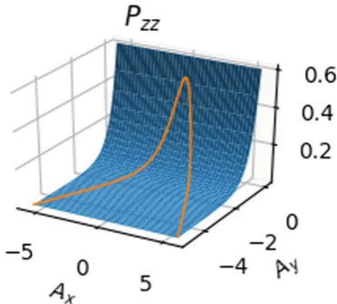
As an example we show a surface plot forP Azz( x,Ay)for

the Harris sheet(figure1). The distribution function used for the plot is F H ps( s, xs,pys)µexp[-bs(Hs-u pys ys)] which

leads to Pzzµexp 2( Ay) with Ay appropriately normalised.

Because the potential Pzzdepends only on one of the

coor-dinates Ax, Ay, the particle will be able to move in the Ax

direction at constant ‘velocity’ corresponding to a constant guidefieldBy=By0. The value of this constant is determined by the initial conditions of the particle motion.

We discuss this analogy to particle motion in a potential in so much detail because it is very useful in addressing the first of the two problems mentioned above, namely tofind out a prioriwhat types of magneticfield profiles are inconsistent with the‘inverse’approach as specified so far. As an example we will use an asymmetric current sheet without guidefield, i.e. with onlyB zx( )¹0. Then, as in the Harris sheet casePzz

will only be a function of Ay. For a particle trajectory to

represent a current sheet, i.e. for the magneticfield to reverse direction, the particle trajectory has to have a turning point where it stops and turns around. However, on a surface depending only on one single variable the return branch of the trajectory has to be the same as the inward part of the tra-jectory, hence ruling out any potential asymmetry. We remark that this changes if a guide field, even if constant, is intro-duced, because that opens up the possibility of making Pzz

dependent on Ax as well (see e.g. [27, 29, 30]). Reasoning

along the same lines one can, for example, rule out repre-senting configurations such as double current sheets with this approach.

[image:3.595.333.519.67.234.2]

The uniqueness problem can be addressed to some extent by restricting the class of distribution function under con-sideration. In his method Channell [26] uses equilibrium

Figure 1.The surface showsP Azz( x,Ay)=exp 2( Ay) 2, representing

the potential surface for the Harris sheet. The yellow line shows the solution(A zx( ),A zy( ))=(z,-ln cosh( ( )))z corresponding to a

distribution functions of the type

F H p p n

v H g p p

, ,

2 exp , , 24

s s xs ys

s s

s s s xs ys

0

th, 3

p b

=

-( )

( ) ( ) ( ) ( )

withvth,s=(bsms)-1 2andn0sa constant with the dimension

of a particle density. Here,gsis an unknown function of the

canonical momenta. Before charge neutrality is imposed,Pzz

has the form

Pzz 1 exp q N A ,A , 25

s s

s s s x y

å

_b b

= (- F) ( ) ( )

with

N A A n

v

m

v v g p p v v

,

2 exp

2 , d d .

26

s x y s s

s s

x y s xs ys x y

0

th,2

2 2

ò ò

p

b =

´ - +

-¥ ¥

-¥ ¥

⎡

⎣⎢ ⎤⎦⎥

( )

( ) ( )

( )

For the method to work one has to ensure thatF =0 which implies that N Ai( x,Ay)=N Ae( x,Ay)=N A( x,Ay) (see e.g.

[3, 31, 32]) for all possible values of Ax, Ay. This imposes

additional conditions which the parameters of the distribution function have to satisfy. The neutralPzzis then given by

P Azz x,Ay e iN A ,A . 27

e i

x y

b b

b b

= +

( ) ( ) ( )

Using the canonical momenta instead of the velocity com-ponents as integration variables and using equation(27),(26)

becomes

N A A n

m v

m p q A p q A

g p p p p

,

2

exp 2

, d d . 28

x y s s s s

s

xs s x ys s y s xs ys xs ys

0 2

th, 2

2 2

ò ò

p

b =

´ - - +

-´

-¥ ¥

-¥ ¥

⎧ ⎨ ⎩

⎫ ⎬ ⎭

( )

[( ) ( ) ]

( ) ( )

For P Azz( x,Ay) a known function of Ax and Ay, this is a

Fredholm integral equation of the first type that has to be solved for the unknown functiong p_s( _xs,p_ys).

We remark that different functional dependences of the distribution function on the Hamiltonian Hs are possible,

leading to integral equations with different kernels. As far as the authors are aware this possibility has not yet been investigated in much detail(except in[33]). One interesting possibility would be to consider an energy dependence leading to Kappa-type distribution functions as in e.g.[25]for the Harris sheet magneticfield.

3. Examples

In his paper, Channell[26] gives a number of examples of how his method could be used tofind distribution functions for given functionsN A( x,Ay). If one would like to start from

a given magnetic field profileB( )z =(B zx( ),B zy( ), 0) there is an additional step that one has to carry out, namely to determineN A( x,Ay)and henceP Azz( x,Ay)from the magnetic

field profile. Thefirst step in this process should of course be to determine the vector potential components A zx( )andA zy( )

for the given magneticfield profile. One can determine how Pzz varies with z along the given trajectory A zx( ),A zy( ) by

using macroscopic force balance which states that

z

B z B z

P z

d

d 2 0. 29

x y

zz

2 2

0 m +

+ =

⎛ ⎝

⎜⎜ ⎞

⎠ ⎟⎟

( ) ( )

( ) ( )

Integrating with respect to zand calling the integration con-stantPT, one gets

P z P B z B z

2 . 30

zz T

x y

2 2

0 m

= - +

( ) ( ) ( ) ( )

Constructing a function of two variables P Azz( x,Ay) defined

over the complete Ax–Ay-plane from knowledge of P zzz( )

along one single trajectory A zx( ),A zy( ) is sometimes

pro-blematic due to the intrinsic non-unique nature of this task, but as we will see later this can also provide opportunities for finding more convenient solutions. We see from equation(30)

that the absolute value of Pzz along the trajectory is

deter-mined only up to a constant, because the value of PT is

arbitrary apart from demanding that P zzz( )has to be positive

for all z. We remark that equations (20) and (21) are con-straints that also have to be satisfied, and imply that along the known trajectory not only Pzz is determined, but also its

gradient. Apart from these constraints the surfaceP Azz( x,Ay)

can in principle be deformed arbitrarily(obviously one needs to ensurePzz>0).

For the remainder of this section we will focus on a particular type of current sheet magnetic fields, the so-called force-free current sheets. Force-free magnetic fields have a current density that is parallel to the magnetic field (jB), i.e. m₀j=aB. Here α can be either a constant, leading to linear force-free fields, or a function of position, leading to nonlinear force-free fields. Under the assumptions made we can have at most a=a( )z . In the context of the ‘inverse’ approach as discussed above the question of what type of

P Azz( x,Ay) functions are consistent with force-free magnetic

fields has been answered in[3]. For force-freefields

z

B z B z

d

d 2 0, 31

x y

2 2

0 m +

=

⎛ ⎝

⎜⎜ ⎞

⎠ ⎟⎟

( ) ( )

( )

which together with the force balance equation(29)gives the condition

P

z

d

d 0, 32

zz ₌

( )

implying that the trajectory A zx( ),A zy( )representing a

force-free solution of Ampèreʼs law has to coincide with a contour of the Pzzsurface.

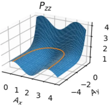
This is, for example, satisfied by Pzz surfaces that are

equivalent to attractive central potentials depending on

Ax2 +Ay2. Such potentials have circular contours and admit

arbitrary phase). Distribution functions leading to linear force-free fields have been known since the 1960ʼs (e.g. [26,

34–39]) and generally have the form F H ps s, xs pys

2 ₊ 2

( ) (see

e.g.[3]).

A distribution function leading to a nonlinear force-free field was first found by Harrison and Neukirch [31]. The magnetic field profile for that case was B( )z = B0(tanh( ) (z , cosh( ))z -1, 0), withB0the constant value of the

magnitude of the magneticfield. This magneticfield profile has been named the force-free Harris sheet, because it has the same B zx( )as the Harris sheet, but a B zy( ) which renders it

force-free. The form ofPzzfound in[31]was

P A A B A

B L

A

B L b

,

2 1 2cos

2

exp 2 , 33

zz x y x

y

02

0 0 0

m

= ⎡ + +

⎣

⎢ ⎛

⎝

⎜ ⎞

⎠

⎟ ⎛

⎝

⎜ ⎞

⎠

⎟ ⎤

⎦ ⎥

( ) ( )

withLa typical length scale(half-width)of the current sheet configuration and b representing a constant background pressure. The background pressure is needed to keep Pzz

positive(seefigure3). The form of the distribution functions for the pressure (33)can be found and is

F n

v H a u p

u p b

2 exp cos

exp . 34

s s s

s s s s xs xs s ys ys s

0

th, 3

p b b

b

=

-+ +

( ) ( )[ ( )

( ) ] ( )

Hereas,bs,uxsanduysare constant parameters of the problem

(the other parameters have been defined before). As discussed in[31,32]the parameters of the distribution functions have to satisfy a number of relations to on the one hand make the macroscopic parameters such as B0,L, andb consistent with

the kinetic parameters and on the other hand to satisfy the neutrality condition N Ae( x,Ay)=N Ai( x,Ay). One very

interesting property of the distribution functions (34)is that they can have multiple maxima in velocity space in both the vxand thevydirections. The existence of multiple maxima in

velocity space can be linked to the width of the current sheet. The condition for the distribution function(34)to have only a single maximum invxwas derived in[32]to be

b u

v u

v

1

2exp 1 . 35

s xs s

xs s

2

th, 2

2

th, 2

> ⎛ +

⎝

⎜⎜ ⎞_⎠⎟⎟⎛_⎝⎜⎜ ⎞_⎠⎟⎟ ( )

One can also show that

u

v

r

L

4 , 36

xs s

g s

2

th,2

, 2

2

= ( )

whererg s, =m vs th,s (eB0)is the thermal gyroradius of species s. If we assume that all parameters exceptLanduxsarefixed,

one sees that a decrease in the current sheet width L corre-sponds to an increase in uxs, which will eventually lead to a

violation of condition(35)and hence multiple maxima in the vxdirection(for a detailed discussion see[32]).

A number of important extensions have been made to this first nonlinear force-free collisionless current sheet equili-brium. The non-uniqueness of the ‘inverse’ approach was shown by Wilson and Neukirch[33]who showed that thePzz

given in equation (33) can be obtained with distribution functions that have a different dependence on the Hamiltonian Hs than in equation (34), but the same dependence on the

canonical momenta. It was also shown in[40]how the force-free Harris sheet distribution function(34)can be generalised to the relativistic regime.

An important extension to previous work was made by Abraham-Shrauner [41], who generalised the approach to a whole family of magneticfield profiles of the form

z B z L k z L k

B( )= 0(sn( ; ), cn( ; ), 0 ,) (37)

[image:5.595.65.265.68.234.2]

where sn ;(x k) and cn ;(x k) are Jacobian elliptic functions, with 0 k 1 the modulus. This magnetic field profile includes the previously known cases of the linear force-free field in the limitk0 and of the force-free Harris sheet in

Figure 2.The surface showsP Azz( x,Ay)µAx2+Ay2+cand the

yellow line shows the solution(A zx( ),A zy( ))=(sin( )z , cos( ))z

corresponding to a(normalised)magneticfield of the formB( )z =(sin( )z , cos( )z , 0).

[image:5.595.80.262.321.496.2]

the limitk1(see e.g.[42]). The functionPzztakes the form

P B b

k

kA

B L k

k

kA

B L

k

kA

B L

2

3 2

1

2 cos

2

1 4

1

1 exp 2

1 4

1

1 exp 2 , 38

zz x

y

y

02

0 2 0

2

0 2

0

m p

= - -

-- +

+ -

-⎜ ⎟

⎜ ⎟

⎡ ⎣

⎢ ⎛

⎝

⎜ ⎞

⎠ ⎟

⎛ ⎝ ⎞⎠

⎛ ⎝ ⎜ ⎞_⎠⎟

⎛ ⎝ ⎞⎠

⎛ ⎝

⎜ ⎞_⎠⎟⎤ ⎦

⎥ ( )

with the distribution function given by

F H p p n H

v

a a k u p k

a k u p a k u p

, , exp

2 cos

exp exp , 39

s s xs ys

s s s s s s s xs xs

s s ys ys s s ys ys

0

th, 3

0 1

2 3

b p

b p

b b

=

-´ +

-+ +

-( ) ( )

( )

[ ( )

( ) ( )] ( )

with ais constant parameters. Not surprisingly, the velocity

space structure of these distribution functions is of similar complexity to that of the force-free Harris sheet.

Another important generalisation to the case of the force-free Harris sheet was made by Kolotkov et al [43]. Dis-tribution functions of the type(34)as well as those derived in [33] not only lead to a constant Pzz along the force-free

solution, but also to a constant particle density and conse-quently to a constant temperature (if defined by the ratio of Pzzand the particle density). However, a constantPzzat the

macroscopic level could also be achieved by letting both the particle density and the temperature vary, but keeping their product constant. This is exactly what was achieved in[43]by using modified distribution functions of the form

F n

v H a u p b

H u p

2 exp cos

exp exp ,

40

s s s

s s s s xs xs s s s s ys ys

0

th, 3 3 2

p g gb gb

b b

= - +

+

-( ) { ( )[ ( ) ]

( ) ( )}

( )

with an additional parameterγintroduced to allow different parts of the distribution function to have different energy dependence (for a similar approach in a different context see e.g.[28,44]). The macroscopic form of P Azz( x,Ay) given in equation (33)

does not change, but some of the relations between microscopic and macroscopic parameters are modified due to the additional dependence of the distribution function onγ.

One of the shortcomings of all nonlinear force-free cases discussed so far is that they all have a plasma beta that is larger than unity (bpl>1; for discussion see e.g. [45]) independently of the choice of parameters, as long as the constraintFs>0 is satisfied. This is unsatisfactory, because force-freefields are usually associated withbpl<1. One can, however, make use of the fact thatP Azz( x,Ay)can be changed

along the lines described above. For force-free cases a mathematical formulation of this property has been given in [3]showing that a functionP Azz( x,Ay)that admits a force-free

solution can be transformed into other functions P A¯ (zz x,Ay)

admitting the same force-free solution by

P A A

P P A A

, 1 , , 41

zz x y

ff

zz x y

y y

= ¢

¯ ( )

( ) ( ( )) ( )

wherePffis the constant value ofPzzon the force-free contour

and y( )x is a function that is arbitrary apart from the con-straint that the expression on the right hand side of equation (41) has to be positive. As noted in [45, 46] a transformation of the form

P

P P P

exp 1 , 42

zz zz ff

0

y = ⎡

-⎣⎢

⎤ ⎦⎥

( ) ( ) ( )

with P0 a positive constant pressure, leads to (using

equation (41)) a transformed value of Pzz on the force-free

contour ofP¯ff =P0, i.e. one can in principle reducebplfor the force-free solution to any value below one. Starting from equation(33), as a function ofAxandAy,P¯zz becomes[45]

P A A P A

B L

A

B L

, exp 1

2 cos

2

2exp 2 1 . 43

zz x y

x

y

0

pl 0

0

b =

+

-⎪

⎪ ⎧ ⎨ ⎩

⎡ ⎣

⎢ ⎛_⎝⎜ ⎞_⎠⎟

⎛ ⎝

⎜ ⎞

⎠

⎟ ⎤

⎦ ⎥⎫⎬

⎭

¯ ( )

( )

This form of P¯zz leads to a much more complicated form of

equation (28) that needs to be solved, resulting in quite complex mathematical problems. In[45,46]a solution in the form of infinite series of Hermite polynomials is found. The authors also show that the series converges for all values of

pl

b , in particular bpl<1, and under which conditions posi-tivity of the resulting distribution function is to be expected. So far, in all parameter regimes accessible to numerical investigation it has been found that the distribution functions have single maxima in velocity space and are not equal to, but similar to Maxwell distributions. This is a very interesting difference to the distribution function (34). It should be emphasised, however, that only a part of all possible para-meter combinations has been explored so far.

To illustrate the transformation method, we will present a different transformation which also leads to force-free solu-tions withbpl<1, but is mathematically less demanding. The transformation we will use is simply

Pzz Pzz, 44

2

y( )= ( )

which leads to

P P

P

2 , 45

zz zz ff

2

=

¯ _{( )}

with transformed valueP¯ff along the force-free contour given by

P P

2 , 46

ff ff

=

¯ ( )

i.e. the transformedbpl will be half of the value of the original pl

equation(33)we get

P A A B

b

A B L

A

B L b

B b b A B L b A B L b A B L A B L A B L A B L , 2 1 1 2 1 2cos 2 exp 2 2 1 1 2 1 8 1 8cos 4 cos 2

2 exp 2 cos 2 exp 2

exp 4 .

47

zz x y

x y

x

x

y x y

y

02

0 0 0

2 0 2 0 2 0 0

0 0 0

0 m m = + + + = + + + + + + + ⎡ ⎣ ⎢ ⎛_⎝⎜ ⎞_⎠⎟ ⎛_⎝⎜ ⎞_⎠⎟ ⎤ ⎦ ⎥ ⎡ ⎣ ⎢ ⎛ ⎝ ⎜ ⎞_⎠⎟ ⎛ ⎝ ⎜ ⎞_⎠⎟ ⎛ ⎝ ⎜ ⎞_⎠⎟ ⎛_⎝⎜ ⎞_⎠⎟ ⎛_⎝⎜ ⎞_⎠⎟ ⎛ ⎝ ⎜ ⎞ ⎠ ⎟⎤ ⎦ ⎥ ¯ ( ) ( )

Solving equation (28) we obtain distribution functions of the form

F n

v

a u p a u p

a u p u p a u p

a u p a

2 e

cos 2 exp 2

cos exp cos

exp , 48 s s s H

s s xs xs s s ys ys

s s xs xs s ys ys s s xs xs s s ys ys s

0 th, 3 1 2 3 4 5 6 s s p b b

b b b

b = ´ + + + + + b -( ) [ ( ) ( ) ( ) ( ) ( ) ( ) ] ( ) with

e u e u

B L e u

e u u u

2

, 49

e xe i xi e ye i yi xs ys

0

b b b

b

- = = =

-=  =

∣ ∣ ∣ ∣

∣ ∣ ( )

n0e=n0i=n0, (50)

n B

b

2 1

1 2 , 51

e i e i 0 0 2 0 b b

b b m

+ ₌ + ( ) a u v a u v

exp 2 exp 2 1

8, 52

e xe th e i xi th i 1 2 , 2 1 2 , 2 - = - = ⎛ ⎝ ⎜⎜ ⎞_⎠⎟⎟ ⎛_⎝⎜⎜ ⎞_⎠⎟⎟ ( ) a u v a u v

exp 2 exp 2 1, 53

e ye th e i yi th i 2 2 , 2 2 2 , 2 = = ⎛ ⎝ ⎜⎜ ⎞_⎠⎟⎟ ⎛_⎝⎜⎜ ⎞_⎠⎟⎟ ( )

a3e=a3i=1, (54)

a u

v a

u

v b

exp

2 exp 2 , 55

e xe e i xi i 4 2 th, 2 4 2 th, 2 - = - = ⎛ ⎝ ⎜⎜ ⎞_⎠⎟⎟ ⎛_⎝⎜⎜ ⎞_⎠⎟⎟ ( ) a u v a u v b exp

2 exp 2 2 , 56

e ye e i yi i 5 2 th,2 5 2 th,2 = = ⎛ ⎝ ⎜⎜ ⎞_⎠⎟⎟ ⎛_⎝⎜⎜ ⎞_⎠⎟⎟ ( )

a a b 1

8, 57

e i

6 = 6 = 2 + ( )

so thatNe=Niand the macroscopic expression forP¯zz matches

the expression calculated from thev_z2moment of the distribution function(48).

One has to ensure that Fs>0 for all pxs, pys and that

leads to certain restrictions on the parameter values if one also wants to ensure thatPff <2. For example, one has to have

b <3 2 and uxi2 vth,2i has to be approximately smaller than

1.2. Contrary to the work by Allanson and co-workers

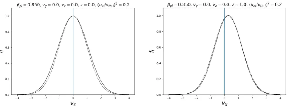
[45, 46], there is no issue with convergence of an infinite series. A preliminary study of the distribution functions for this case for bpl<1 has only found distribution functions which have a single maximum in velocity space and seem to be quite close to Maxwellian distribution functions (see figure4 for an example). Further and more detailed investi-gations will have to be carried out to see whether this is the case for all parameter combinations withbpl<1or whether there are cases withbpl<1and distributions functions with multiple maxima in velocity space. We would like to emphasise that while the transformation consists simply of squaringPzz, it is not the case that the distribution function is

simply squared as well. By trial and error, we have found some examples of multi-peaked distribution functions for transformed cases withbpl>1, but the plasma beta had to be greater than approximately 2.5. Due to the larger number of terms in the distribution function for the transformed case it is not at all clear whether an analytical criterion such as equation(35)for the original, untransformed case, can also be found for the transformed case. Also, no immediate conclu-sions for the distribution function of the transformed case can be drawn from the fact that the distribution function for the untransformed case can have multiple maxima. However, for the case shown infigure4, the parameterbsin equations(34)

and(35)corresponds toa6sin equation(48). If we choose the

same parameters as used infigure 4for the transformed case in the original distribution function(34) (settingbs=a6s), we

would find that the original distribution function would also only have a single maximum in vx. As stated above, the

possible parameter choices for the transformed case are to some extent influenced by the fact that the distribution functions have to be positive and one could speculate that this restriction might play a role in the possible velocity space structures of the distribution functions. It is definitely inter-esting that so far all equilibrium distribution functions that have been investigated for the cases of the force-free Harris sheet magnetic fields with abpl<1have a relatively simple structure in velocity space, but it is too early to conclude that this is always the case.

4. Discussion and conclusions

In this paper we have presented a general overview of rela-tively recent work on the ‘inverse’problem for collisionless current sheet equilibria, focussing on one-dimensional force-free equilibria in Cartesian coordinates. A natural question is whether this can be extended to other geometries, e.g. rota-tionally symmetric equilibria representing flux tubes and some work in this direction has been undertaken[5,6].

An important application for collisionless current sheet models are plasma and magneticfield structures in planetary magnetospheres and a large amount of work on collisionless equilibria in general has been done in this area (see e.g. [2, 8, 10, 29] for overviews and [5, 10, 47–51] for recent work).

processes such as magnetic reconnection(e.g.[52]). In many cases the Harris sheet with a constant guidefield is used as the underlying equilibrium but force-free magnetic field confi g-urations have recently been used more often as starting point for investigations, for example using particle-in-cell (PIC) simulations. PIC simulations starting with linear force-free fields and the corresponding exact equilibrium distribution functions have been carried out by a number of authors (see e.g.[39, 53–56]). Simulations have also been done for the force-free Harris sheet, but usually with initial distribution functions that are Maxwell–Boltzmann distributions shifted by the macroscopic bulk flow of the particle species (e.g. [57–63]. Other authors used the bi-Maxwellian self-consistent equilibrium distribution function for linear force-free fields (e.g [34, 35, 39]) to initialise their simulations (e.g. [64, 65]). The equilibrium distribution function for the force-free Harris sheet found in[31]has been used as initial equilibrium for PIC simulations in[66](see also [56]). It is interesting that the results of most of these simulations with regards to the properties of collisionless reconnection agree despite the differences in the simulation set-up both regarding the initial conditions and the simulation parameters.

On the other hand, the results by Allanson and co-workers[45,46] as well as the(preliminary)results for the quadratic transformation presented in this paper seem to suggest that there are equilibrium distribution functions for the force-free Harris sheet in the regime withbpl<1that do not deviate massively from shifted Maxwellian distribution functions. This could explain why a set-up using shifted Maxwellians might be justified, although this needs to be investigated in more detail in the future.

One other interesting question that would be worth addressing in the future concerns the non-uniqueness of the ‘inverse’ problem. In particular, in cases where several dis-tribution functions are known for the same magnetic field profile, it would be interesting to know which of those

distribution functions is in any way ‘preferred’. A first step would be a linear stability analysis and one would intuitively assume that, for example, multi-peaked distribution functions would be subject to micro-instabilities. However, it would also be of value to think about criteria which would help to select equilibrium distribution functions according to, for example, a (nonlinear)energy principle.

Acknowledgments

The authors acknowledge financial support by the UK Sci-ence and Technology Facilities Council Consolidated Grants ST/K000950/1 and and ST/N000609/1, as well as Doctoral Training Grant ST/K502327/1. OA also acknowledges support by the UK Natural Environment Research Council Grant NE/P017274/1.

ORCID iDs

T Neukirch https://orcid.org/0000-0002-7597-4980

References

[1] Biskamp D 2000Magnetic Reconnection in Plasmas (Cambridge, UK: Cambridge University Press) [2] Schindler K 2007Physics of Space Plasma Activity

(Cambridge: Cambridge University Press)

[3] Harrison M G and Neukirch T 2009Phys. Plasmas16022106 [4] Kocharovsky V V, Kocharovsky V V, Martyanov V Y and

Tarasov S V 2017Phys.—Usp. 591165

[image:8.595.57.548.67.250.2]

[5] Vinogradov A A, Vasko I Y, Artemyev A V, Yushkov E V, Petrukovich A A and Zelenyi L M 2016Phys. Plasmas23 072901

Figure 4.Plot of the distribution function(48)for ions againstvx(withvy=vz=0)forz=0(left panel)andz=1.0(right panel). The distribution function has been normalised so that its maximum is one. The parameter values used in these plots areb=1.2,

b

0.5 0.5 0.85

pl

b = ( + )= andu vxi2 th,-2i=0.2. For comparison the dashed line in each plot shows a Maxwellian distribution function with a

[6] Allanson O, Wilson F and Neukirch T 2016Phys. Plasmas23 092106

[7] Schindler K and Birn J 2002J. Geophys. Res.(Space Phys.)

10720-1

[8] Zelenyi L M, Malova H V, Artemyev A V, Popov V Y and Petrukovich A A 2011Plasma Phys. Rep.37118–60 [9] Mingalev O V, Mingalev I V, Mel’nik M N, Artemyev A V,

Malova H V, Popov V Y, Chao S and Zelenyi L M 2012 Plasma Phys. Rep.38300–14

[10] Artemyev A and Zelenyi L 2013Space Sci. Rev.178419–40 [11] Vasko I Y, Artemyev A V, Popov V Y and Malova H V 2013

Phys. Plasmas20022110

[12] Tasso H and Throumoulopoulos G 2014Eur. Phys. J.D

68175

[13] Catapano F, Artemyev A V, Zimbardo G and Vasko I Y 2015 Phys. Plasmas22092905

[14] Davidson R C 2001Physics of Nonneutral Plasmas (Singapore: World Scientific)

[15] Kropotkin A P and Domrin V I 1996J. Geophys. Res.101 19893–902

[16] Kropotkin A P, Malova H V and Sitnov M I 1997J. Geophys. Res.10222099–106

[17] Sitnov M I, Zelenyi L M, Malova H V and Sharma A S 2000 J. Geophys. Res.10513029–44

[18] Sitnov M I, Guzdar P N and Swisdak M 2003Geophys. Res. Lett.3045-1

[19] Artemyev A V 2011Phys. Plasmas18022104 [20] Grad H 1961Phys. Fluids41366–75

[21] Belmont G, Aunai N and Smets R 2012Phys. Plasmas19 022108

[22] Dorville N, Belmont G, Aunai N, Dargent J and Rezeau L 2015Phys. Plasmas22092904

[23] Mynick H E, Sharp W M and Kaufman A N 1979Phys. Fluids

221478–84

[24] Harris E G 1962Nuovo Cimento23115

[25] Fu W Z and Hau L N 2005Phys. Plasmas12070701 [26] Channell P J 1976Phys. Fluids191541–5

[27] Alpers W 1969Astrophys. Space Sci.5425–37 [28] Mottez F 2003Phys. Plasmas102501–8

[29] Roth M, de Keyser J and Kuznetsova M M 1996Space Sci. Rev.76251–317

[30] Allanson O, Neukirch T, Hodgson J, Wilson F and Liu Y H 2017Geophys. Res. Lett.448685–95

[31] Harrison M G and Neukirch T 2009Phys. Rev. Lett.102 135003

[32] Neukirch T, Wilson F and Harrison M G 2009Phys. Plasmas

16122102

[33] Wilson F and Neukirch T 2011Phys. Plasmas18082108 [34] Moratz E and Richter E W 1966Z. Nat.forsch.A211963 [35] Sestero A 1967Phys. Fluids10193–7

[36] Bobrova N A and SyrovatskiǐS I 1979Sov. J. Exp. Theor. Phys. Lett.30535

[37] Correa-Restrepo D and Pfirsch D 1993Phys. Rev.E47545–63 [38] Attico N and Pegoraro F 1999Phys. Plasmas6767–70 [39] Bobrova N A, Bulanov S V, Sakai J I and Sugiyama D 2001

Phys. Plasmas8759–68

[40] Stark C R and Neukirch T 2012Phys. Plasmas19012115 [41] Abraham-Shrauner B 2013Phys. Plasmas20102117

[42] NIST Digital Library of Mathematical Functionshttp://dlmf. nist.gov/, Release 1.0.9 of 2014-08-29 online companion to [67]http://dlmf.nist.gov/

[43] Kolotkov D Y, Vasko I Y and Nakariakov V M 2015Phys. Plasmas22112902

[44] Génot V, Mottez F, Fruit G, Louarn P, Sauvaud J A and Balogh A 2005Planet. Space Sci.53229–35

[45] Allanson O, Neukirch T, Wilson F and Troscheit S 2015Phys. Plasmas22102116

[46] Allanson O, Neukirch T, Troscheit S and Wilson F 2016 J. Plasma Phys.82905820306

[47] Panov E V, Artemyev A V, Nakamura R and Baumjohann W 2011J. Geophys. Res.(Space Phys.)116A12204

[48] Malova H V, Popov V Y, Mingalev O V, Mingalev I V, Mel’nik M N, Artemyev A V, Petrukovich A A,

Delcourt D C, Shen C and Zelenyi L M 2012J. Geophys. Res.(Space Phys.)117A04212

[49] Artemyev A V, Vasko I Y and Kasahara S 2014Planet. Space Sci.96133–45

[50] Vasko I Y, Artemyev A V, Petrukovich A A and Malova H V 2014Ann. Geophys.321349–60

[51] Petrukovich A, Artemyev A, Vasko I, Nakamura R and Zelenyi L 2015Space Sci. Rev.188311–37 [52] Hesse M, Neukirch T, Schindler K, Kuznetsova M and

Zenitani S 2011Space Sci. Rev.1603–23

[53] Li H, Nishimura K, Barnes D C, Gary S P and Colgate S A 2003Phys. Plasmas102763–71

[54] Nishimura K, Gary S P, Li H and Colgate S A 2003Phys. Plasmas10347–56

[55] Bowers K and Li H 2007Phys. Rev. Lett.98035002 [56] Harrison M 2009 Equilibrium and dynamics of collisionless

current sheetsPhD ThesisThe University of St Andrews (https://research-repository.st-andrews.ac.uk/bitstream/ handle/10023/705/Michael%20G.%20Harrison%20PhD% 20thesis.PDF?)

[57] Hesse M, Kuznetsova M, Schindler K and Birn J 2005Phys. Plasmas12100704

[58] Liu Y H, Daughton W, Karimabadi H, Li H and Roytershteyn V 2013Phys. Rev. Lett.110265004 [59] Guo F, Li H, Daughton W and Liu Y H 2014Phys. Rev. Lett.

113155005

[60] Guo F, Liu Y H, Daughton W and Li H 2015Astrophys. J.

806167

[61] Liu Y H, Hesse M and Kuznetsova M 2015J. Geophys. Res. (Space Phys.)1207331–41

[62] Guo F, Li X, Li H, Daughton W, Zhang B, Lloyd-Ronning N, Liu Y H, Zhang H and Deng W 2016Astrophys. J. Lett.818L9 [63] Guo F, Li H, Daughton W, Li X and Liu Y H 2016Phys.

Plasmas23055708

[64] Zhou F, Huang C, Lu Q, Xie J and Wang S 2015Phys. Plasmas22092110

[65] Fan F, Huang C, Lu Q, Xie J and Wang S 2016Phys. Plasmas

23112106

[66] Wilson F, Neukirch T, Hesse M, Harrison M G and Stark C R 2016Phys. Plasmas23032302