Replicable parallel branch and bound search

Replicable parallel branch and bound search

ARCHIBALD, Blair, MAIER, Patrick <http://orcid.org/0000-0002-7051-8169>,

MCCREESH, Ciaran, STEWART, Robert and TRINDER, Phil

Available from Sheffield Hallam University Research Archive (SHURA) at:

http://shura.shu.ac.uk/18625/

This document is the author deposited version. You are advised to consult the

publisher's version if you wish to cite from it.

Published version

ARCHIBALD, Blair, MAIER, Patrick, MCCREESH, Ciaran, STEWART, Robert and

TRINDER, Phil (2018). Replicable parallel branch and bound search. Journal of

Parallel and Distributed Computing, 113, 92-114.

Copyright and re-use policy

See

http://shura.shu.ac.uk/information.html

Contents lists available atScienceDirect

J. Parallel Distrib. Comput.

journal homepage:www.elsevier.com/locate/jpdc

Replicable parallel branch and bound search

Blair Archibald

a,

*

,

Patrick Maier

a

,

Ciaran McCreesh

a

,

Robert Stewart

b

,

Phil Trinder

a

a_{School Of Computing Science, University of Glasgow, Scotland, G12 8QQ, United Kingdom} b_{Heriot-Watt University, Edinburgh, Scotland, EH14 4AS, United Kingdom}

h i g h l i g h t s

• We consider how to gain replicable performance for parallel branch and bound searches.

• We provide a reduction-oriented formal model of parallel branch and bound.

• We present a generic branch and bound API based around higher order functions.

• We design two parallel skeletons each with different performance characteristics.

• Evaluation shows that the Ordered skeleton achieves both good and replicable parallel performance.

a r t i c l e i n f o

Article history:

Received 20 February 2017 Received in revised form 17 July 2017 Accepted 15 October 2017

Keywords:

Algorithmic skeletons Branch-and-bound Parallel algorithms Combinatorial optimisation Distributed computing Repeatability

a b s t r a c t

Combinatorial branch and bound searches are a common technique for solving global optimisation and decision problems. Their performance often depends on good search order heuristics, refined over decades of algorithms research. Parallel search necessarily deviates from the sequential search order, sometimes dramatically and unpredictably, e.g. by distributing work at random. This can disrupt effective search order heuristics and lead to unexpected and highly variable parallel performance. The variability makes it hard to reason about the parallel performance of combinatorial searches.

This paper presents a generic parallel branch and bound skeleton, implemented in Haskell, with replicable parallel performance. The skeleton aims to preserve the search order heuristic by distributing work in an ordered fashion, closely following the sequential search order. We demonstrate the generality of the approach by applying the skeleton to 40 instances of three combinatorial problems: Maximum Clique, 0/1 Knapsack and Travelling Salesperson. The overheads of our Haskell skeleton are reasonable: giving slowdown factors of between 1.9 and 6.2 compared with a class-leading, dedicated, and highly optimised C++ Maximum Clique solver. We demonstrate scaling up to 200 cores of a Beowulf cluster, achieving speedups of 100x for several Maximum Clique instances. We demonstrate low variance of parallel performance across all instances of the three combinatorial problems and at all scales up to 200 cores, with median Relative Standard Deviation (RSD) below 2%. Parallel solvers that do not follow the sequential search order exhibit far higher variance, with median RSD exceeding 85% for Knapsack.

©2017 The Author(s). Published by Elsevier Inc. This is an open access article under the CC BY license (http://creativecommons.org/licenses/by/4.0/).

1. Introduction

Branch and bound backtracking searches are a widely used class of algorithms. They are often applied to solve a range of NP-hard optimisation problems such as integer and non-linear programming problems; important applications include frequency planning in cellular networks and resource scheduling, e.g. assign-ing deliveries to routes [26].

*

Corresponding author.

E-mail addresses:[email protected](B. Archibald), [email protected](P. Maier),[email protected] (C. McCreesh),[email protected](R. Stewart),[email protected] (P. Trinder).

Branch and bound systematically explores asearch treeby sub-dividing the search space and branching recursively into each sub-space. The advantage of branch and bound over exhaus-tive enumeration stems from the way branch and boundprunes branches that cannot better theincumbent, i.e. the current best solution, potentially drastically reducing the number of branches to be explored.

The effectiveness of pruning depends on two factors: (1) the accuracy of the problem-specific heuristic to compute bounds (2) the value of optimal solutions in each branch, and on the quality of the incumbent; the closer to optimal the incumbent, the more can be pruned. As a result, branch and bound is sensitive tosearch order, i.e. to the order in which branches are explored.

https://doi.org/10.1016/j.jpdc.2017.10.010

A good search order can improve the performance of branch and bound dramatically by finding a good incumbent early on, and highly optimised sequential algorithms following the branch and bound paradigm often rely on very specific orders for performance. Branch and bound algorithms are hard to parallelise for a num-ber of reasons. Firstly, while branching creates opportunities for speculative parallelism where multiple workersi.e threads/pro-cessors search particular branches in parallel, pruning counter-acts this, limiting potential parallelism. Secondly, parallel pruning requires that processors share access to the incumbent, which limits scalability. Thirdly, parallel exploration of irregularly shaped search trees generates unpredictable numbers of parallel tasks, of highly variable duration, posing challenges for task scheduling. Finally, and most importantly, parallel exploration alters the search order, potentially impacting the effectiveness of pruning.

As a result of the last point in particular, parallel branch and bound searches can exhibit unusual performance characteristics. For instance, slowdowns can arise when the sequential search finds an optimal incumbent quickly but the parallel search delays ex-ploring the optimal branch. Alternately, super-linear speedups are possible in case the parallel search happens on an optimal branch that the sequential search does not explore until much later. In short, the perturbation of the search order caused by adding pro-cessors makes it impossible topredictparallel performance.

These unusual performance characteristics make reproducible algorithmic research into combinatorial search difficult: was it the new heuristic that improved performance, or were we just lucky with the search ordering in this instance? As the instances we wish to tackle become larger, parallelism is becoming central to algorithmic research, and it is essential to be able to reason about parallel performance.

This paper aims to develop a generic parallel branch and bound search for distributed memory architectures such as clusters. Cru-cially, the objective ispredictable parallel performance, and the key to achieving this is careful control of the parallel search order.

The paper starts by illustrating performance anomalies with parallel branch and bound by using a Maximum Clique graph search. The paper then makes the following research contribu-tions:

•

To address search order related performance anomalies, Section2postulates threeparallel search propertiesfor repli-cable performance as follows.

Sequential Bound: Parallel runtime is never higher than sequential (one worker) runtime.

Non-increasing Runtimes: Parallel runtime does not in-crease as the number of workers inin-creases.

Repeatability: Parallel runtimes of repeated searches on the same parallel configuration have low variance.

•

We define a novel formal model for general parallel branch and bound backtracking search problems (BBM) that spec-ifies both search order and parallel reduction (Section3). We show the generality of BBM by using it to define three different benchmarks with a range of application areas: Maximum Clique (Section3), 0/1 Knapsack (Appendix B) and Travelling Salesperson (Appendix D).

•

We define a new Generic Branch and Bound (GBB) search API that conforms to the BBM (Section4). The generality of the GBB is shown by using it to implement Maximum Clique (Section 2),1 _{0/1 Knapsack (Appendix C) and Travelling}

Salesperson (Appendix E).

1_{This implementation being the firstdistributed-memoryparallel}

[image:3.595.397.477.52.140.2]

implementa-tion of San Segundo’s bit parallel Maximum Clique algorithm (BBMC) [52].

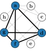
Fig. 1.A graph, with its Maximum Clique{a,d,f,g}shown.

•

To avoid the significant engineering effort required to pro-duce a parallel implementation for each search algorithm we encapsulate the search behaviours as a pair ofalgorithmic skeletons, that is, as generic polymorphic computation pat-terns [12], providing distributed memory implementations for the skeletons (Section5). Both skeletons share the same API yet differ in how they schedule parallel tasks. The Un-ordered skeletonrelies on random work stealing, a tried and tested way to scale irregular task-parallel computations. In contrast, theOrdered skeletonschedules tasks in an ordered fashion, closely following the sequential search order, so as to guarantee the parallel search properties.

•

We compare the sequential performance of the skeletons with a class leading hand tuned C++ search implementation, seeing slowdown factors of between 1.9 and 6.2. We then assess whether the Ordered skeleton preserves the parallel search properties using 40 instances of the three benchmark searches on a cluster with 17 hosts and 200 workers (Section

7). The Ordered skeleton preserves all three properties and produces replicable results. The key results are summarised and discussed in Section8.

2. The challenges of parallel branch and bound search

We start by considering a branch and bound search application, namely finding the largest clique within a graph. The Maximum Clique problem appears as part of many applications such as in bioinformatics [16], in biochemistry [9,15,18,24], for community detection [66], for document clustering [41], in computer vision, electrical engineering and communications [8], for image compar-ison [53], as an intermediate step in maximum common subgraph and graph edit distance problems [34], and for controlling flying robots [48].

To illustrate the Maximum Clique problem we use the example graph inFig. 1. In practice the graphs searched are much larger, having hundreds or thousands of vertices. A clique within a graph is a set of vertices where each vertex in the set is adjacent to every other vertex in the set. For example, inFig. 1the setV

= {

a

,

b

,

c

}

is a clique as all vertices are adjacent to one another.

{

a

,

b

,

h

}

is not a clique as there is no edge betweenbandh. In the Maximum Clique problem we wish to find a largest clique (there may be multiple of the same size) in the graph. Here we are interested in theexact solution requiring the full search space to be explored.

One approach to solving this problem would be to enumerate the power set of vertices and check the clique property on each (ordering by largest set). While this approach can work for smaller graphs, the number of combinations grows exponentially with the number of nodes in the graph making it computationally unfeasi-ble for large graphs.

vertices adjacent to all vertices in the current clique. Once there are no valid branching choices left we can record the size of the clique andbacktrack.

Finally, we can go one step further with the addition of bound-ing. The idea of bounding is that acurrent best result, known as the incumbent, is maintained. For Maximum Clique this corre-sponds to the size of the largest clique seen so far. At each step we determine, using a bounding function, whether or not the current selection of vertices and those remaining could possibly unseat the incumbent and if it is impossible then backtracking can occur, reducing the size of the search space. For the Maximum Clique example the maximum size, given a current clique, may be estimated using a greedy colouring algorithm: clearly, if we can colour the remaining vertices usingkcolours (giving adjacent vertices different colours), then the current clique cannot be grown by more thankvertices.

Practical algorithms for the Maximum Clique problem were the subject of the second DIMACS implementation challenge in 1993 [22]. In 2012, Prosser [47] performed a computational study of exact maximum clique algorithms, focusing on a series of al-gorithms using a colour bound [58–60], together with bit-parallel variants [52,55] that represent adjacency lists using bitsets to gain increased performance via vectorised instructions. Since then, ongoing research has looked at variations on these algorithms, including reordering colour classes [36], reusing colourings [40], treating certain vertices specially [56], and giving stronger (but more expensive) bounding using rules based upon MaxSAT in-ference between colour classes [27,28,54]. (A recent broader re-view [64] considers both heuristic and exact algorithms.)

There have been three thread-parallel implementations of these algorithms [15,35,37], the most recent makes use of detailed inside-search measurements to explain why parallelism works, and how to improve it. These studies have been limited to multi-core systems. A fourth study [65] attempted to use MapReduce on a similar algorithm, but only presented speedup results on three of the standard DIMACS instances, all of which possess special properties which make parallelism unusually simple [37].

For simplicity this paper uses a bit-parallel variant of the MCSa1 algorithm [47], which is BBMC [52] with a simpler initial vertex ordering. Crucially the algorithm is not straightforward, and that unlike the naïve and overly simplistic algorithms typically used to demonstrate skeletons, is both close to the state of the art and a realistic reflection of modern practical algorithms.

2.1. General branch and bound search

Although we introduced branch and bound search in relation to the Maximum Clique problem, it has much wider applications. It is commonly seen for global optimisation problems [39] where some property is either maximised or minimised within a general search space. Two other examples where branch and bound search may be used are given in Sections6.1and6.2.

The details and descriptions of these algorithms vary and we take a unifying view using terminology from constraint program-ming. In general, a constraint satisfaction or optimisation problem has a set of variables, each with a domain of values. The goal is to give each variable one of the values from its domain, whilst re-specting all of a set of constraints that restrict certain combinations of assignments. In the case of optimisation problems, we seek the best legal assignment, as determined by some objective function.

Such problems may be solved by some kind of backtracking search. Branch and bound is a particular kind of backtracking search algorithm for optimisation problems, where the best solu-tion found so far (theincumbent) is remembered, and is used to prune portions of the search space based upon an over-estimate (theboundfunction) of the best possible solution within an unex-plored portion of the search space.

For example, when searching for a Maximum Clique (a subset of vertices, where every vertex in the set is adjacent to every other in the set) in a graph, we have a ‘‘true or false’’ variable for each vertex, with true meaning ‘‘in the clique’’. We may branch on whether or not to include any given vertex, reject any undecided vertices that are not adjacent to the vertex we just accepted, and then bound the remaining search space using the colour bound mentioned above. In practice, selecting a good branching rule makes a huge differ-ence. We must select a variable, and then decide the value to assign it first. There are good general principles for variable selection, but value ordering tends to be more difficult in practice.

2.2. Parallelisation and search anomalies

Search algorithms have strong dependencies: before we can evaluate a subtree, we need to know the value of the incum-bent from all the preceding subtrees so we can determine if the bound can eliminate some work. Parallelism in these algorithms isspeculativeas it ignores the dependencies and creates tasks to explore subtrees in parallel. This approach can lead to anomalous performance, and specifically.

1. When subtrees are explored in parallel some work may be wasted, since we might be exploring a subtree that would have been pruned in a sequential run by a stronger incum-bent. As the parallel version is performing more work than the sequential version, its runtime may exceed that of the sequential version.

2. Conversely, it may be that a parallel task finds a strong incumbent more quickly than in the sequential execution, leading to less work being done. In this case we observe superlinear speedups.

3. An absolute slowdown, where the parallel version runs ex-ponentially slower than a sequential run. This can happen if introducing parallelism alters the search order, leading to it taking longer for a strong incumbent to be found.

The theoretical conditions where these three conditions can occur are well-understood [14,25,29,61]. In particular, it is possible to guarantee that absolute slowdowns will never happen, by re-quiring parallel search strategies to enforce certain properties [14].

2.3. Implementation challenges

The most obvious complicating factor when parallelising a branch and bound search tree is irregularity: it is extremely hard to decompose the problem up-front to do static work allocation, since some subproblems are exponentially more complicated than others.

To deal with irregular subproblems efficiently we require a form of dynamic load balancing that can re-assign problems to cores as they become idle. A common approach to dynamic load balancing in parallel search [42] (and general parallelism) is throughwork stealing: we start with a sequential search, but allow additional workers to ‘‘steal’’ portions of the search space and explore them in parallel. Popular off-the-shelf work stealing systems commonly employ a randomised stealing strategy, which has good theoretical properties [7].

factor in the results. We expect that as core counts increase, such factors will become even more important.

From an implementation perspective, anomalies cause serious complications, with inconsistent and hard-to-understand speedup results being common. Randomised work stealing schemes fur-ther complicate matters and recent research [11,37,38] has demonstrated a connection between value-ordering heuristic be-haviour [20] and parallel work splitting strategies that explains anomalous behaviour. We now understand why randomised work stealing behaves so erratically in practice in these settings: it in-teracts poorly with carefully designed search order strategies [37]. For consistently strong results, we cannot think of parallelism inde-pendently of the underlying algorithm, and must instead use work stealing to explicitly offset the weakest value ordering heuristic behaviour. For this reason, the best results for parallel Maximum Clique algorithms currently come from handcrafted and complex work distribution mechanisms requiring extremely intrusive mod-ifications to algorithms. It is not surprising that these implementa-tions are currently restricted to a single multi-core machine.

To conduct replicable parallel branch and bound research it is essential to avoid these anomalies. To do so we propose that parallel branch and bound search implementations should meet the following properties.2

Sequential Bound: Parallel runtime is never higher than se-quential (one worker) runtime.

Non-increasing Runtimes: Parallel runtime does not increase as the number of workers increases.

Repeatability: Parallel runtimes of repeated searches on the same parallel configuration have low variance.

Engineering a parallel implementation that ensures these prop-erties for each search algorithm is non-trivial, and hence in Section

5we develop generic algorithmic branch and bound skeletons, which greatly simplify the implementation of parallel searches.

3. A formal model of tree traversals

This section formalises parallel backtracking traversal of search trees with pruning, modelling the behaviour of a multi-threaded branch-and-bound algorithm in the reduction style of operational semantics. This formal model, for brevity referred to asBBM, ad-mits reasoning about the effects of parallel reductions, in particular how parallelism affects the potential to prune the search space.

Reduction-based operational semantics of algorithmic skele-tons has been studied previously [3] for standard stateless skele-tons like pipelines and maps. BBM does not fit this stateless framework since branch and bound skeletons maintain state in the form a globally shared incumbent. There are several theoretical analyses of parallel branch and bound search [6], often specific to a particular search algorithm. BBM is novel in encoding generic branch and bound searches as a set of parallel reduction rules.

3.1. Modelling trees and tree traversals

In practice, search trees are implicit. They are not materialised as data structures in memory but traversed in a specific order, for instance depth-first. In contrast, for the purpose of this formali-sation we assume the search tree is fully materialised. This is not a restriction as the search tree is typically generated by a tree generator. In practice, the tree generator is interleaved with the tree traversal avoiding the need to materialise the search tree in memory.

2_{We are interested in parallel searches that meet or fail to meet these properties}

due to search order effects. We ignore resource related effects such as problem size being too small or massive oversubscription.

We formalise trees as prefix-closed sets of words. To this end, we introduce some notation. LetXbe a non-empty set. By 2X_{, we}

denote the power set ofX. We denote the set of finite words over alphabetXbyX∗_{, and the empty word by}

ϵ

_{. We write}

|

w

|

_{to denote}

the length of a word

w

∈

X∗_.

We denote the prefix order onX∗_by

⪯

_{. By}

≤

lex, we denote the

lexicographic extension of the natural order

≤

onNtoN∗. Note that

≤

lexis an extension of the prefix order

⪯

, that is, being

prefix-ordered implies being prefix-ordered lexicographically on words inN∗_.

Trees. Atree T over alphabet Xis a non-empty subset ofX∗_such

that there is a least (w. r. t. the prefix-order) elementu

∈

T, andT is prefix-closed aboveu. Formally,Tis prefix-closed aboveuif for all

v, w

∈

X∗_,u

⪯

v

⪯

w

_and

w

∈

_Timplies

v

∈

_{T. WhenXandu}

are understood, we will simply callT atree. We call the elements ofT vertices. We call the least elementu

∈

T theroot; and we call

v

∈

Taleaf if it is maximal w. r. t. the prefix order, that is, if there is no

w

∈

Twith

v

≺

w

. We call two distinct vertices

w, w

′

∈

_T

siblingsif there are

v

∈

X∗_anda

,

_a′

∈

_{Xsuch that}

w

=

v

_aand

w

=

v

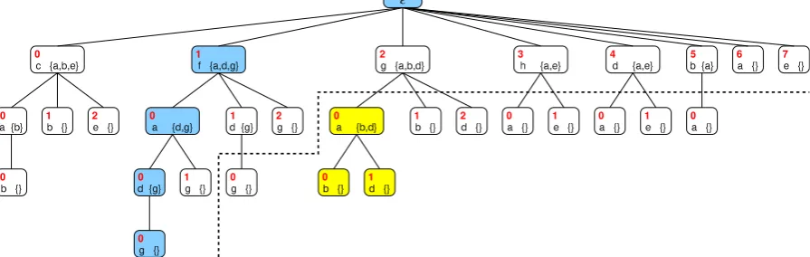
a′_.

Fig. 2depicts an example tree over the natural numbers. That is, each vertex corresponds to the unique sequence of red numbers from the root

ϵ

. For example, the blue leaf is vertex 1000, whereas the yellow non-leaf is vertex 20.

We call a functiong

:

X∗

→

₂X _{atree generator. Given such}

a tree generatorg, we definetg as the smallest subset ofX∗that

contains

ϵ

and is closed underg in the following sense: For all u

∈

tg and alla

∈

g(u),ua

∈

tg. Clearly,tg is a tree with root

ϵ

,

thetree generated byg.

Subtrees and segments. LetT be a tree. A subsetSof vertices ofT is asubtreeofT ifS is a tree. Given a vertexu

∈

T, we call the greatest (with respect to set inclusion) subtreeSofT with rootu thesegmentofTrooted atu. The yellow vertices inFig. 2depict the segment

{

20

,

200

,

201

}

, rooted at vertex 20.

Two segments of T are overlapping if they intersect non-trivially, in which case one is contained in the other. A set of segmentscoverthe treeTif the prefix-closure of their union equals T. That is, if for eachu

∈

Tthere is a segmentSand

v

∈

Ssuch that u

⪯

v

.

Ordered trees. Trees as defined above capture the parent–child relation (via the prefix order on words) but do not impose any order on siblings. Yet, many tree traversals rely on a specific order on siblings. To be able to express such an order, we generalise the notion of trees toorderedtrees. We do so by labelling trees over the natural numbers, using the usual order of the naturals (or rather, its lexicographic extension to words) to order siblings.

Formally, anordered tree

λ

over Xis a function

λ

:

dom(

λ

)

→

X∗

such that

•

dom(

λ

) is a tree overN_,

•

the image of

λ

is a tree overX, and

•

λ

is an order isomorphism between the two trees, both ordered by the prefix order

⪯

.

Since

λ

is an isomorphism of the prefix order the lengths of the wordsuand

λ

(u) coincide for allu

∈

dom(

λ

). In an abuse of notation, we write

λ

to denote both the ordered tree (i. e. the function fromdom(

λ

) toX∗_{) as well as the corresponding tree over}

X(i. e. the image of the function

λ

). WhenXis understood, we will simply call

λ

an(ordered) tree. To avoid confusion, we will call the elements of

λ

vertices, and the elements ofdom(

λ

)positions.

[image:6.595.70.518.57.199.2]

Fig. 2.Depiction of an ordered tree. The path in blue identifies the leaf 1000; the vertices in yellow make up the tree segment rooted at 20. The vertices below the dashed line are cut off by a sequential branch and bound traversal. (For interpretation of the references to colour in this figure legend, the reader is referred to the web version of this article.)

the alphabetX

= {

a

, . . . ,

h

}

, where

λ

maps each position to the string of black letters from the root to the corresponding node. For instance

λ

maps position 1000 to the stringfadgwhich happens to represent the maximum clique of the graph inFig. 1.

As

λ

is an order isomorphism the lexicographic ordering on dom(

λ

) carries over to the tree

λ

. That is, we define for allu

, v

∈

dom(

λ

),

λ

(u)

≤

lex

λ

(

v

) if and only ifu

≤

lex

v

, and

≤

lexbecomes a

total ordering on

λ

.

We call a functiong

:

X∗

→

_X∗_{anordered tree generatorif all}

images ofgare isograms, i. e. have no repeating letters. Given an ordered tree generatorg, we define

λ

_g

:

dom(

λ

_g)

→

X∗ _{as the}

function with smallest domain such that

•

dom(

λ

_g) is a tree overN,

•

λ

g(

ϵ

)

=

ϵ

, and

•

λ

_gis closed undergin the following sense: For all positions u

∈

dom(

λ

_g) and corresponding vertices

v

=

λ

_g(u), ifg(

v

)

=

a0a1

. . .

an−1andi

<

nthenuiis a position indom(

λ

g) and

λ

_g(ui)

=

v

ai.

By construction

λ

g is an order isomorphism as images ofgare

isograms, hence

λ

_g is an ordered tree,theordered tree generated byg.

Example: Tree generators for clique problems. LetG

= ⟨

V

,

E

⟩

be an undirected graph. Given a vertexu

∈

V, we denote its set of neighbours byE(u).

We defineg

:

V∗

→

₂V _byg(u

1

. . .

um)

= {

v

∈

V

| ∀

i

:

v

̸=

ui

∧

ui

∈

E(

v

)

}

. Clearly,g is a generator for the treetg

over the alphabetX

=

V, enumerating all cliques ofG. However, tg enumerates cliques as strings rather than sets and hence every

clique of sizekwill be enumeratedk

!

times.

To avoid enumerating the same clique multiple times, we need to generate an ordered tree where siblings ‘‘to the right’’ avoid vertices that have already been chosen ‘‘on the left’’. We construct an ordered tree over the alphabetX

=

V

×

2V_{, where the first}

component is the latest vertex added to the current clique and the second component is a set of candidate vertices that may extend the current clique. The candidate vertices are incident to all vertices of the current clique, but do not necessarily form a clique themselves. We define the ordered tree generatorh

:

X∗

→

_X∗_by

h(

⟨

u1

,

U1

⟩

. . .

⟨

um

,

Um

⟩

)

= ⟨

v

1

,

V1

⟩

. . .

⟨

v

n

,

Vn

⟩

such that

•

the

v

ienumerate the setU, and

•

theVi

=

(U

\ {

v

1

, . . . , v

i−1

}

)

∩

E(

v

i)

whereU

=

Umifm

>

0, andU

=

Votherwise. Typically, the

⟨

v

_i

,

Vi

⟩

are ordered such that the size ofVidecreases asiincreases;

this order is beneficial for sequential branch and bound traversals.

Clearly,his an ordered generator for an ordered tree enumer-ating all cliques ofG exactly once(ignoring the second component of the alphabet).Fig. 2shows a tree generated byhfor the graph fromFig. 1.

3.2. Maximising tree traversals

The trees defined above materialise the search space and order traversals. What is needed for modelling branch-and-bound is an objective functionto be computed during traversal that the search aims to maximise.

LetYbe a set with a total quasi-order

⊑

, that is

⊑

is a reflexive and transitive, but not necessarily anti-symmetric, total binary relation onY.

Given a treeT overXand anobjectivefunctionf

:

X∗

→

_Y,

the goal is to maximisef overT, i. e. to find someu

∈

T such that f(u)

⊒

f(

v

) for all

v

∈

T. The objective function is required to be monotonic w. r. t. the prefix order, that is for allu

,

u′

∈

_X∗_{, ifu}

⪯

_u′

thenf(u)

⊑

f(u′_{). By monotonicityf(}

ϵ

_{) is a minimal element of the}

image off.

So far, we have modelled maximising tree search. To model branch-and-bound we introduce one additional refinement: A predicatepforpruningsubtrees that cannot improve the incum-bent. More precisely, thepruningpredicatep

:

Y

×

X∗

→ {

₀

,

₁

}

is a function mapping the incumbent (i. e. the maximal value off seen so far) and the current vertex to 1 (forprune) or 0 (forexplore). The pruning predicate must satisfy the following monotonicity and compatibility conditions:

1. For ally

∈

Yandu

,

u′

∈

_X∗_{, ifu}

⪯

_u′_thenp(y

,

_u)

≤

_p(y

,

_u′_).

2. For ally

,

y′

∈

_Yandu

∈

_X∗_{, ify}

⊑

_y′_thenp(y

,

_u)

≤

_p(y′

,

_u).

3. For ally

∈

Yandu

∈

X∗_{, ifp(y}

,

_u)

=

_{1 thenf(u)}

⊑

_y.

Condition 1 implies that all descendantsu′_{of a pruned vertexu}

are also pruned. Condition 2 implies a vertex pruned by incumbent yis also pruned by any stronger incumbenty′_{. Finally, Condition 3}

states the correctness of pruning w. r. t. maximising the objective function: Vertexuis pruned by incumbentyonly iff(u) does not beaty.

Example: Objective function and pruning predicate for clique prob-lems. For maximum clique, we setY

=

N_{, and the quasi-order}

⊑

is the natural order

≤

. We define the objective functionf

:

X∗

→

_Y

byf(

w

)

= |

w

|

. That is, maximisingf means finding cliques of maximum size. We define the pruning predicatep

:

Y

×

X∗

→

{

0

,

1

}

by

p(l

,

⟨

_

,

U1

⟩

. . .

⟨

_

,

Um

⟩

)

=

{

1 ifm

>

0 andm

+ |

Um

| ≤

l

0 otherwise

That is, pruning decisions rest on the size of the current clique,m, and the size of the set of remaining candidate verticesUm; vertices

will be pruned if adding these two sizes does not exceed the current boundl.3

3.3. Modelling multi-threaded tree traversals

For this section, we fix an ordered tree

λ

overX, which we will traverse according to the order

≤

lex. We also fix an objective

functionf

:

X∗

→

_{Y, and a pruning predicatep}

:

_Y

×

_X∗

→ {

₀

,

₁

}

_,

whereYis a set with a total quasi-order

⊑

. Finally, we fix a setSEG of pairwise non-overlapping tree segments that cover the tree

λ

; we call each segmentS

∈

SEGatask.

State. Let n

≥

1 be the number of threads. The state of a backtracking tree traversal is a (n

+

2)-tuple of the form

σ

=

⟨

x

,

Tasks

, θ

₁

, . . . , θ

_n

⟩

, where

•

x

∈

λ

is theincumbent, i. e. the vertex that currently max-imisesf,

•

Tasks

∈

SEG∗_{is a queue of pending tasks, and}

•

θ

_iis the state of theith thread, where

θ

_i

= ⊥

if theith thread is idle, or

θ

_i

= ⟨

Si

, v

i

⟩

ifSi

∈

SEGis theith thread’s current

task and

v

_i

∈

Sithe currently explored vertex of that task.

We use Haskell list notation for the task queueTasks. That is,

[ ]

denotes the empty queue, andS

:

Tasksdenotes a non-empty queue with headS

∈

SEG.

The initial state is

⟨

ϵ,

Tasks

,

⊥

, . . . ,

⊥⟩

, where the list Tasks enumerates all tasks inSEG, in an arbitrary but fixed order. Afinal stateis of the form

⟨

x

,

[ ]

,

⊥

, . . . ,

⊥⟩

.

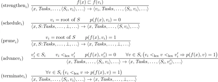
Reductions. The reduction rules inFig. 3define a binary relation

→

on states. Each rule carries a subscript indicating which thread it is operating on. Rule (strengthen_i) is applicable if theith thread is not idle and its current vertex

v

ibeats the incumbent onf. Of

the remaining four rules exactly one will be applicable to theith thread (unless a final state is reached).

Rules (schedulei) and (prunei) apply if the ith thread is idle

and the task queue is non-empty. Which of the two rules applies depends on whether the root vertex

v

iof the head taskSin the

queue is to be pruned or not. If not,S becomes theith thread’s current task and

v

_ithe current vertex, otherwise taskSis pruned and theith thread remains idle.

Rules (advancei) and (terminatei) apply if the ith thread is

not idle. Which of the two rules applies depends on whether all vertices of the current taskSibeyond the current vertex

v

i(in the

lexicographic order

<

lex) are to be pruned according to predicate

p. If so, theith thread terminates the current task and becomes idle, otherwise the thread advances to the next vertex

v

′

i that is

not pruned.

It is easy to see that no rule is applicable if and only if all threads are idle and the task queue is empty, that is, iff a final state is reached.

3_{More accurate pruning can be achieved by replacing the size ofU}

mwith the

size of the maximum clique of the subgraph induced byUm; greedily colouring this

subgraph makes for an efficient approximation of maximum clique size.

Admissible reductions.

The reduction rules inFig. 3do not specify an ordering on the rules nor stipulate any restriction on the relative speed of execu-tion of different threads. However, applying the rules in just any order is too liberal. In particular, not selecting rule (strengtheni)

when the incumbent could in fact be strengthened may result in missing the maximum. To avoid this, rule (strengthen_i) must be prioritised as follows.

We call a reduction

σ

→

σ

′ _{inadmissible if it uses rule}

(advancei) or (terminatei) even though rule (strengtheni) was

ap-plicable in state

σ

. A reduction isadmissibleif it is not inadmissi-ble. Admissible reductions prioritise rule (strengtheni) over rules

(advancei) and (terminatei).

By induction on the length of the reduction sequence, one can show that an incumbent x maximises the objective function f over the ordered tree

λ

whenever

⟨

x

,

[ ]

,

⊥

, . . . ,

⊥⟩

is a final state reachable from the initial state

⟨

ϵ,

Tasks

,

⊥

, . . . ,

⊥⟩

by a sequence of admissible reductions.

We point out that final states are generally not unique. For in-stance, a graph may contain several different cliques of maximum size, and a parallel maxclique search may non-deterministically return any of these maximum cliques. Therefore the reduction relation cannot be confluent.

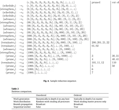
Example: Reductions for maxclique. Consider the tree inFig. 2 en-coding the graph inFig. 1. LetTasks

= [

S0

,

S1

,

S2

,

S3

,

S4

,

S5

,

S6

,

S7

]

be a queue of tasks such thatSi is the segment rooted at vertex

i; for example the segmentS2 is determined by the set of

po-sitions

{

2

,

20

,

200

,

201

,

21

,

22

}

. Clearly, theSiare pairwise

non-overlapping and cover the whole tree. In Fig. 4, we consider a sample reduction with three threads (with IDs 1 to 3) following a strict round-robin thread scheduling policy, except for selecting the strengthening ruleeagerly(that is, as soon as it is applicable). For convenience, we display the reduction rule used in the left-most column and index the reduction arrow with the number of reductions.

We observe that up to reduction 11, the three threads traverse the search tree segmentsS0,S1andS2in parallel. From reduction

12 onwards, the incumbent is strong enough to enable pruning according to the heuristic, i.e. prune if size of current clique plus number of candidates does not beat size of the incumbent. Column prunedlists the positions of the search tree where traversal stopped due to pruning; columncut off list the positions that were never reached due to pruning. The reduction illustrates that parallel traversals potentially do more work than sequential ones in the sense that fewer positions are cut off. Concretely, thread 3 tra-verses segmentS2because the incumbent is too weak; a sequential

traversal would have entered S2 with the final incumbent and

pruned immediately, as indicated by the dashed line inFig. 2. The reduction also illustrates that parallelism may reduce runtime: a sequential traversal would explore firstS0and thenS1, whereas

thread 2 locates the maximum clique inS1without traversingS0

first.

4. Generic branch and bound search

This section uses the model in Section3as the basis of a Generic Branch and Bound (GBB) API for specifying search problems. The GBB API makes extensive use of higher-order functions, i.e. func-tions that take funcfunc-tions as arguments, and hence is suitable for parallel implementation in the form of skeletons (Section5).

We introduce each of the GBB API functions, give their types and show an example of how to use them in a simple implementation of the Maximum Clique problem (Section2). Later sections show that the API is general enough to encode other branch and bound applications (Sections6.1and6.2).

[image:8.595.80.503.55.214.2]

Fig. 3.Reduction rules.

1 -- application dependent types

2 typeSpace -- data (e.g. graph) relevant to the problem

3 typePartialSolution -- partial solution of the problem

4 typeCandidates -- set of candidates for extending the partial solution

5 typeBound -- "size" of the partial solution; instance of Ord

6

7 -- type of nodes making up the search tree

8 typeNode=(PartialSolution, Bound, Candidates)

9

10 -- generates a list of candidate Nodes for extending the search tree by

11 -- extending the PartialSolution of the given Node with each of the Candidates

12 orderedGenerator :: Space →Node → [Node]

13

14 -- Returns an upper bound on the size of any solution that could result

15 -- from extending the given Node’s PartialSolution with any of the given

16 -- Candidates

17 pruningHeuristic :: Space →Node → Bound

Listing 1: Generic Branch and Bound (GBB) search API

4.1. Types

The fundamental type for a search is aNode that represents a single position within a search tree (for example inFig. 2each box represents a node). This notion of a node differs slightly from the BBM where a single type,X∗_{, is used to uniquely identify a}

particular tree node by the branches leading to it. For an effi-cient implementation, rather than store an encoding of the branch through the tree, the node type uses the partial solution to encode the branch history and the candidate set to encode potential next steps in the branch. The current bound is maintained for efficiency reasons but could alternatively be calculated from the current solution as in the BBM.

The abstract types are described below, and Table 1 shows how the abstract types map to implementation specific types for Maximum Clique (Section2), Knapsack (Section6.1) and Travelling Salesperson (Section6.2) searches.

Space: Represents the domain specific structure to be searched. Solution: Represents the current (partial) solution at this node.

The solution is an application specific representation of a branch within the tree and encodes the history of the search.

Candidates: Represents the set of candidates that may still be added to the solution to extend the search by a single step. This may be used to encode implementation specific details such as no non-adjacent nodes in a maximum clique search, or simply ensure that no variable is chosen twice. It is not required that the type of the candidates matches the type the search space.

This enables implementation-specific optimisations such as the bitset encoding found in the BBMC algorithm (Section7.1.1). Bound: Represents the bound computed from the current

so-lution. There must be an ordering on bounds, for example as provided by Haskell’s Ord typeclass instance [19] to allow a maximising tree traversal to be performed implicitly using the type.

Node: Represents a position within the search space. For effi-ciency it caches the current bound, current solution and can-didates for expansion.

4.1.1. Function usage

It is perhaps surprising that the application specific aspects of a branch and bound search can be both precisely specified, and efficiently implemented, with just two functions. The GBB API functions rely on the implicit ordering on the bound type, but could easily be extended to take an ordering function as an argument.

orderedGenerator: generates the set of candidate child nodes from a node in the space. Search heuristics can be encoded by ordering the child nodes in a list. The search ordering may use these heuristics to provide simple in-order tree traversal or more elaborate heuristics such as depth based discrepancy search (Section7.1.1).

[image:9.595.44.293.501.647.2]

Table 1

Abstract to concrete type mappings.

Abstract type Maximum Clique Knapsack TSP

Space Graph List of all Items DistanceMatrix

Solution List of chosen vertices List of chosen items Current (partial) Tour Candidates Vertices adjacent to all solution vertices All remaining items All remaining cities Bound Size of the current chosen vertices list Current profit of items Current tour length

These functions correspond to the branching and bounding functions respectively. We chose to call themorderedGeneratorand pruningHeuristicto highlight their purposes: to generate the next steps in the search and to determine if pruning should occur.

Listing2shows instances of these GBB functions that encode a simple,IntSetbased, version of the Maximum Clique search. The orderedGeneratorbuilds a set of candidate nodes based on a greedy graph colouring algorithm (colourOrder). The colourings provide a heuristic ordering and, by storing them alongside the solution’s vertices, allow effective bounding to be performed. Candidates only include vertices that are adjacent to every vertex already in the clique. ThepruningHeuristicchecks if the number of vertices in the current clique and potential colourings can possibly unseat the incumbent. See Section7.1.1for instances of the GBB API that use a more realistic bitset encoding [52,55].

4.2. General branch and bound search algorithm

The essence of a branch and bound search is a recursive function for traversing the nodes of the search space. Algorithm1shows the function expressed in terms of the GBB API (Listing1) where we assume that the incumbent and associated bound are read and written by function calls rather than being explicitly passed as arguments and returned as a result. Hence the final solution is read from the global accessor function instead of the algorithm returning an explicit value. As we are dealing with maximising tree traversals, bounds are always compared using agreater than(

>

) function defined on theBoundtype.

Parallelism may be introduced by searching the set of candi-datesspeculativelyin parallel, as illustrated in Section5. Parallel search branches allow early updates of the incumbent via (glob-ally) synchronised versions of the currentBound and updateBest functions.

expandSearch

(space, node) begin

candidates = orderedGenerator(space, node) ifnull(candidates)then

return

// Backtrack

// Parallelism may be introduced here

forc in candidatesdo

bestBound = currentBound()

localBest = pruningHeuristic(space, node) iflocalBest

>

bestBoundthen

ifbound(node)

>

bestBoundthen

updateBest(solution(node), bound(node)) expandSearch(space, c)

return

// Backtrack

Algorithm 1:General algorithm for branch and bound search using the GBB API (Listing1).

currentBound

and

updateBest

are built-in functions

4.3. Implementing the GBB API

Although GBB can encode general branch and bound searches, various modifications improve both sequential and parallel effi-ciency.

Generally the search space is immutable and fixed at the start of the search. In a distributed environment we can avoid copying the search space each time a task is stolen by storing a read only copy of the search space on each host. It is also possible to remove the space argument from the API functions and add accessor functions in the same manner as bound access. The implementations used in Section7do pass the space as a parameter.

For some applications, such as Maximum Clique, if the local bound fails to unseat the incumbent then all other candidate nodes to-the-right (assuming an ordered generator) will also fail the pruning predicate. An implementation can take advantage of this fact and break the candidate checking loop for an early backtrack. This optimisation is key in avoiding wasteful search. In the skeleton implementations used in Section7we allow this behaviour to be toggled via a runtime flag.

Finally, an implementation can exploit lazy evaluation within the node type to avoid redundant computation. Taking Maximum Clique as an example we can delay the computation of the set of candidates vertices until after the pruning heuristic has been checked (as this only depends on having the bound and colour). Similarly if we use the to-the-right pruning optimisation, described above, we want to avoid paying the cost of generating the nodes which end up being pruned.

5. Parallel skeletons for branch and bound search

Algorithmic skeletons are higher order functions that abstract over common patterns of coordination and are parameterised with specific computations [12]. For example, a parallel map function will apply a sequential function to every element of a collection in parallel. Skeletons are polymorphic, so the collection may contain elements of any type, and the function type must match the ele-ment type. The programmer’s task is greatly simplified as they do not need to specify the coordination behaviour required. The skele-ton model has been very influential, appearing in parallel standards such as MPI and OpenMP [10,57], and distributed skeletons such as Google’s MapReduce [13] are core elements of cloud computing.

Here the focus is on designing skeletons for maximising branch and bound search on distributed memory architectures. These ar-chitectures use multiple cooperating processes with distinct mem-ory spaces. The processes may be spread across multiple hosts.

Although it is possible to implement skeletons using a variety of parallelism models, we adopt a task parallel model here. The task parallel model is based around breaking down a problem into multiple units of computation (tasks) that work together to solve a particular problem. In a distributed setting, tasks (and their results) may be shared between processes. For search trees, parallel tasks generally take the form of sub-trees to be searched.

Two skeleton designs are given in this section. The first skeleton, Unordered, makes no guarantees on the search ordering and so may give the anomalous behaviours and the unpredictable parallel performance outlined in Section2.2. The second skeleton,Ordered, enforces a strict search ordering and hence avoids search anoma-lies and gives predictable performance. The unordered skeleton is used as an example of the pitfalls of using a standard random work stealing approach and provides a baseline comparison for evaluating the performance of the Ordered skeleton (Section7).

1 typeVertex=Int 2 typeVertexSet=IntSet

3 typeColour=Int 4

5 typeSpace =Graph

6 typePartialSolution=([Vertex], Colour)

7 typeCandidates=VertexSet

8 typeBound=Int

9 typeNode =(PartialSolution, Bound, Candidates)

10

11 colourOrder :: Graph→ VertexSet → [(Vertex, Colour)]

12 colourOrder=-- defined elsewhere

13

14 -- Reduce a list to a value of type b

15 foldl :: (b →a → b) → b → [a]→ b

16 foldl f accumulator [] =accumulator

17 foldl f accumulator (x:xs)=foldl (f accumulator x) xs

18

19 orderedGenerator :: Graph →Node → [Node]

20 orderedGenerator graph ((clique, colour), candidates, size)=

21 let choices=colourOrder graph candidates

22 in fst(foldl buildNodes ([], candidates) choices)

23 where

24 buildNodes :: ([Node], VertexSet) → (Vertex, Colour) → ([Node], VertexSet)

25 buildNnodes (nodes, candidates) (v, colour)=let 26 newClique=(v : clique, colour - 1)

27 newSize =size+1

28 newCandidates =VertexSet.intersection candidates (adjVertices graph v)

29 -- We delete v from candidates to avoid generating duplicate solutions

30 -- from any vertex "to-the-left" of the current

31 in (nodes++[(newClique, newSize, newCandidates)], VertexSet.delete v candidates)

32

33 pruningHeuristic :: Graph →Node → Bound

34 pruningHeuristic g ((clique, colour), bnd, candidates)=bnd+colour

Listing 2: Maximum Clique problem using the GBB API

Unordered skeleton can be constructed, and then show the mod-ifications required to transform the Unordered into the Ordered skeleton. Section5.4summarises the design choices and limita-tions of the design choices are summarised in Section5.5.

5.1. Design choices

Three main questions drive the design of branch and bound search skeletons:

1. How is work generated?

2. How is work distributed and scheduled? 3. How are the bounds propagated?

The first two choices focus on task parallel aspects of the design and are common design features for algorithmic skeletons. Bound propagation is a specific issue for branch and bound search and takes the form of a general coordination issue rather than being tied to the task parallel model.

To achieve performance in the task parallel model, tasks should be oversubscribed, that is there should be more tasks than cores, while avoiding low task granularity where communication and synchronisation overheads may outweigh the benefits of the par-allel computation. To achieve these characteristics in the skeleton designs a simple approach for work generation is used: generate parallel tasks from the root of the tree until a given depth threshold is reached. This method exploits the heuristic that tasks near the top of the tree are usually of coarse granularity than those nearer the leaves, i.e. they have more of the search space to consider. This threshold approach is commonly used in divide-and-conquer parallelism and allows a large number of tasks to be generated while avoiding low granularity tasks. The argument that tasks near

the top of the tree have coarse granularity does not necessarily hold true for all branch and bound searches as variant candidate sets and pruning can truncate some searches initiated near the root of the tree: hence task granularity may be highly irregular.

5.2. Unordered skeleton

The type signature of the Unordered skeleton is:

search :: Int -- Depth to spawn to -- Root node

→Node Sol Bnd Candidates

-- orderedGenerator

→(Space →Node Sol Bnd Candidates

→ [Node Sol Bnd Candidates])

-- pruningHeuristic

→(Space →Node Sol Bnd Candidates

→Bool)

→Par Solution

In the skeleton search tasks recursively generate work, i.e. new search tasks. If the depth of a search task does not exceed the threshold it generates new tasks on the host, otherwise the task searches the subtree sequentially.

The current incumbent, i.e. best solution, is held on every host, and managed by a distinguished master process. Bound propaga-tion proceeds in two stages. Firstly when a search task discovers a new Solution it sends both the solution and bound to the master and, if no better solution has yet been found, they replace the incumbent. Secondly the master broadcasts the new bound to all other processes, that update their local incumbent unless they have located a better solution. This is a form of eventual consistency [62] on the incumbent. Using this approach, as opposed to fully peer to peer, the new solution is sent to the master once and only bounds are broadcast. While broadcast is bandwidth intensive, broadcast-ing new bounds provides fast knowledge transfer between search tasks. Moreover experience shows that often agood, although not necessarily optimal, bound is found early in the search making bound updates rare. In many applications the bounds are range-limited, e.g. a Maximum Clique cannot be larger than the number of vertices in the graph.

5.3. Ordered skeleton

The type signature of the Ordered skeleton is as follows.

search :: Bool-- Diversify search → Int -- Depth to spawn to -- Root node

→ Node Sol Bnd Candidates

-- orderedGenerator

→ (Space → Node Sol Bnd Candidates

→ [Node Sol Bnd Candidates])

-- pruningHeuristic

→ (Space → Node Sol Bnd Candidates

→ Bool)

→ Par Solution

The additional first parameter enables discrepancy search or-dering (Section7.1.1) to be toggled; an alternative formulation would be to pass an ordering function in explicitly. The skeleton adapts the Unordered skeleton to avoid search anomalies (Section

2.2) and give predictable performance properties as shown in Sec-tion1.

The Sequential Bound property guarantees that parallel run-times do not exceed the sequential runtime. To maintain this property we enforce that at least one worker executes tasks in the exact same order as the sequential search. The other workers spec-ulatively execute other search tasks and may improve the bound earlier than in the fully sequential case, as illustrated inFig. 4. Discovering a better incumbent early enables the sequential thread to prune more aggressively and hence explore less of the tree than the entirely sequential search would, providing speedups. While there is no guarantee that the speculative workers will improve the bound, the property will still be maintained by the sequential worker.

Requiring a sequential worker is a departure from the fully random work stealing model. Instead of all workers performing random steals, the task scheduling decisions are enforced for the sequential worker. Our system achieves sequential ordering by du-plicating the task information. One set is stealable by any worker, and the other is restricted to the sequential worker. There is a chance that work will be duplicated as some worker may simulta-neously attempt to start the same task as the sequential worker. To avoid duplicating work, we use a basic locking mechanism where workers first check whether a task has already started execution before starting the task themselves.

With random scheduling adding a worker may disrupt a good parallel search order (Section 2.2), so to guarantee the non-increasing runtimesproperty we need to preserve the parallel search order, just as the sequential worker preserves the sequential search order. Preserving the parallel search order means that if withnworkers we locate an incumbent by timetpn, then with

n

+

1 workers we locate the same incumbent, or a better incum-bent, at approximatelytpn. The approximation is required as, in a

distributed setting,tpnmay vary slightly due to the speed of bound

propagation.

It transpires that preserving the parallel search order is also suf-ficient to guarantee therepeatabilityproperty as all parallel exe-cutions follow very similar search orders. The parallel search order must be globally visible for it to be preserved, and we can no longer permit random work stealing. Instead all tasks are generated on the master host and maintained in a centralpriorityqueue. In our skeleton implementation we use depth-bounded work generation to statically construct a fixed set of tasks, with set priorities, before starting the search. Alternative work generation approaches, for example dynamic generation, are possible provided all tasks are generated on the master host.

The parallel search order may have dramatic effects on search performance [11,37,38]. In our skeletonsanyfixed ordering will maintain the properties, although it may not guarantee good per-formance. The GBB API in Section4relies on the user choosing an ordering of nodes in theorderedGeneratorfunction. This ordering is generally, but not necessarily, based on some domain specific heuristic. One simple scheduling decision, and our default, is to assign priorities from left-most to right-most task in the tree. The skeleton may use any priority order rather than the default left-to-right order, for example the depth-bounded discrepancy (DDS) order [63]. This discrepancy ordering is used when evaluating the Maximum Clique benchmark (Section7.1.1).

By augmenting the Unordered skeleton with a single worker that follows the sequential ordering and a global priority ordering on tasks we arrive at the Ordered skeleton that provides reliable performance guarantees while still enabling parallelism.

5.4. Skeleton comparison

Table 2compares the key design features of the two skeletons. A key difference is where tasks are generated and stored. The Unordered skeleton adopts a dynamic approach at the cost of not giving the same performance guarantees as the Ordered skeleton due to a lack of global ordering. Many other skeleton designs are possible. An advantage of the skeleton approach that exploits a general API is that parallel coordination alternatives may be explored and evaluated without refactoring the application code.

5.5. Limitations

For most design choices we have selected a simple alternative. More elaborate alternatives might well deliver better performance. Here we discuss some of the limitations imposed by the simple alternatives selected.

[image:12.595.98.484.52.406.2]

Fig. 4.Sample reduction sequence.

Table 2

Skeleton comparison.

Unordered Ordered

Work generation Dynamically to depthdon any host Statically to depthdon master Work distribution Random work stealing all processes Work stealing master process only Bounds propagation Broadcast Broadcast

Sequential worker False True

A consequence of static work generation in the Ordered skele-ton is that the runtime for the single worker case can be larger than that of a fully sequential search implementation. With static work generation, work is generated from nodes at a depthdahead of time and the parent nodes are no longer considered (as they are already searched). This leads to the creation of additional tasks that a sequential implementation may never create due to prun-ing at the higher levels. The management and searchprun-ing of these additional tasks causes the discrepancy between the single worker Ordered skeleton and purely sequential search. While this does not effect the properties, as we phrase property 1 in terms of a single worker, it would if a purely sequential implementation in property 1 is considered. The effects of this limitation could be mitigated by treating all nodes above the depth threshold as tasks and allowing cancellation of parent/child tasks. Such an approach complicates the task coordination greatly as tasks require knowledge of both their parent and child task states.

The Ordered skeleton requires additional memory and process-ing time on the master host to maintain the global task list and respond promptly to work stealing requests. In practice we have not found this to be a significant issue as most tasks near to top of the search tree are long running and the steals occur at irregular intervals. On large distributed systems, and for some searches, it is possible that a single master might prove to be a scalability bottleneck.

5.6. Implementation

The Ordered and Unordered skeletons are implemented in Haskell distributed parallel Haskell(HdpH) embedded Domain Spe-cific Language (DSL) [30]. HdpH has been modified to use a

priority queue based scheduler to enable the strict ordering on task execution. While HdpH cannot match the performance of the state of the art branch and bound search implementations it is useful for evaluating the skeletons for the following reasons.

1. HdpH supports the higher order functions, a commonly used approach for constructing skeletons.

2. The HdpH is small and easy to modify, allowing ideas to be rapidly prototyped. For example we experimented with priority-based work stealing.

3. The properties of the Ordered skeleton depend on relative runtime values, i.e. absolute runtime is not the priority.

Although our skeletons have been implemented in a func-tional language they may be implemented in any system with the following features: task parallelism; work stealing (random/ single-source); locking; priority based work-queues/task ordering. Distributed memory skeleton implementations will also require distribution mechanisms and distributed locking.

5.7. Maximum Clique representation

To end this section we show, using the functions and types defined in Listing2, how the search skeletons are used within an application. Here we show how the skeleton is called for the Maximum Clique benchmark (Section2):

Unordered.search spawnDepth

(Node ([], 0), 0, allVertices) orderedGenerator

Ordered.search

True-- Use discrepancy search

spawnDepth

(Node ([], 0), 0, allVertices) orderedGenerator

pruningHeuristic

5.8. Other branch and bound skeletons

While algorithmic skeletons are widely used in a range of areas from processing large datasets [13] to multicore programming [49] there has been little work on branch and bound skeletons. Two no-table exceptions are MALLBA [2] and Muesli [45] that both provide distributed branch and bound implementations. Both frameworks are written in C++. Muesli uses a similar higher-order function approach to ourselves while MALLBA is designed around using classesandpolymorphismto override solver behaviour. In Muesli it is possible to choose between a centralised workpool approach, similar to the Ordered skeleton but using work-pushing rather than work stealing, or a distributed method. Unfortunately the centralised workpool model does not scale well compared with our approach (Section7). MALLBA similarly uses a single, centralised, workqueue for its branch and bound implementation. The real strength of the MALLBA framework is in the ability to encode multiple exact and inexact combinatorial skeletons as opposed to just branch and bound.

The Muesli authors further highlight the need for repro-ducible runtimes and note ‘‘the parallel algorithm behaves non-deterministically in the way the search-space tree is explored. In order to get reliable results, we have repeated each run 100 times and computed the average runtimes’’ [45]. By adopting the strictly ordered approach in this paper we avoid the need for large num-bers of repeated measurements to account for non-deterministic search ordering.

6. Model, API and skeleton generality

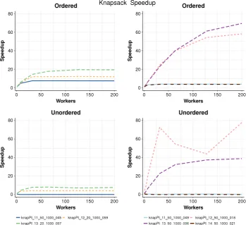
To show that the BBM model and GBB API are generic, and to provide additional evidence that the Ordered skeleton preserves the parallel search properties (Section 7) we consider two ad-ditional search benchmarks: 0/1 Knapsack, a binary assignment problem, and Travelling Salesperson, a permutation problem.

6.1. 0/1 Knapsack

Knapsack packing is a classic optimisation problem. Given a container of some finite size and a set of items, each with some size and value, which items should be added to the container in order to maximise its value? Knapsack problems have important applications such as bin-packing and industrial decision making processes [51]. There are many variants of the knapsack prob-lem [32], typically changing the constraints on item choice. For example we might allow an item to be chosen multiple times, or fractional parts of items to be selected. We consider the 0/1 knapsack problem where an item may only be selected once and fractional items are not allowed.

At each step a bound may be calculated using a linear relaxation of the problem [33] where, instead of solving fori

∈ {

0

,

1

}

we instead solve fractional knapsack problem wherei

∈ [

0

,

1

]

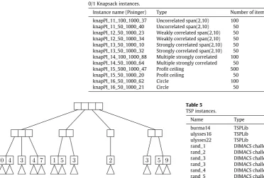
. As the greedy fractional approach is optimal and provides an upper bound on the maximum potential value. Although it is possible to compute an upper bound on the entire computation by considering the choices at the top level [31], we do not implement this here. The primary benefit of this method is to terminate the search early when a maximal solution is found. [image:13.595.312.560.72.110.2]

A formalisation of the 0/1 Knapsack problem in BBM and the corresponding GBB implementation are given in Appen-dices BandCrespectively.

Table 3

Maximum Clique instances.

brock400_1 brock800_1 MANN_a45 sanr200_0.9 brock400_2 brock800_2 p_hat1000–2 sanr400_0.7 brock400_3 brock800_3 p_hat500–3

brock400_4 brock800_4 p_hat700–3

6.2. Travelling Salesperson problem

Travelling Salesperson (TSP) is another classic optimisation problem. Given a set of cities to visit and the distance between each city find the shortest tour where each city is visited once and the salesperson returns to the starting city. We consider only symmetricinstances where the distance between two cities is the same travelling in both directions.

A formalisation of TSP in BBM and the corresponding GBB implementation are given inAppendices DandErespectively.

7. Parallel search evaluation

This section evaluates the parallel performance of the Ordered and Unordered generic skeletons. It starts by outlining the bench-mark instances (Section 7.1) and experimental platform (Sec-tion7.2). We establish a baseline for the overheads of the generic skeletons by comparing them with a state of the art C++ imple-mentation (Section7.3) of Maximum Clique. Finally we investigate the extent that the Ordered skeleton preserves the runtime and repeatability properties (Section2.3) for the three benchmarks.

The datasets supporting this evaluation are available from an open access archive [4].

7.1. Benchmark instances and configuration

This section specifies how the benchmarks are configured and the instances used. We aim for test instances with a runtime of less than an hour while avoiding short sequential runtimes that do not benefit from parallelism. These instances ensure we (a) have enough parallelism and (b) can perform repeated measurements while keeping computation times manageable.

7.1.1. Maximum Clique

The Maximum Clique implementation (Section 2) measured uses the bit set encoded algorithm of San Segundo et al.: BBMC [52,

55]. This algorithm makes use of bit-parallel operations to im-prove performance in the greedy colouring step (orderedGenerator in the GBB API), and ours is the first known distributed parallel implementation of BBMC. We do not use the additional recolouring algorithm [52]. Maxi