A 15 7 minute AM CVn binary discovered in K2

warwick.ac.uk/lib-publications

Original citation:

Green, Matthew J., Hermes, J. J., Marsh, T. R., Steeghs, D., Bell, Keaton J., Littlefair, S. P.,

Parsons, S. G., Dennihy, E., Fuchs, J. T., Reding, J. S., Kaiser, B. C., Ashley, R. P., Breedt, E.,

Dhillon, V. S., Gentile Fusillo, N. P., Kerry, P. and Sahman, D. I. (2018) A 15.7-minute AM CVn

binary discovered in K2. Monthly Notices of the Royal Astronomical Society, 477 (4). pp.

5646-5656. doi:10.1093/mnras/sty1032

Permanent WRAP URL:

http://wrap.warwick.ac.uk/104393

Copyright and reuse:

The Warwick Research Archive Portal (WRAP) makes this work by researchers of the

University of Warwick available open access under the following conditions. Copyright ©

and all moral rights to the version of the paper presented here belong to the individual

author(s) and/or other copyright owners. To the extent reasonable and practicable the

material made available in WRAP has been checked for eligibility before being made

available.

Copies of full items can be used for personal research or study, educational, or not-for-profit

purposes without prior permission or charge. Provided that the authors, title and full

bibliographic details are credited, a hyperlink and/or URL is given for the original metadata

page and the content is not changed in any way.

Publisher’s statement:

This is a pre-copyedited, author-produced PDF of an article accepted for publication in

Monthly Notices of the Royal Astronomical Society following peer review. The version of

record.

Link to final published version:

http://dx.doi.org/10.1093/mnras/sty1032

A note on versions:

The version presented here may differ from the published version or, version of record, if

you wish to cite this item you are advised to consult the publisher’s version. Please see the

‘permanent WRAP URL’ above for details on accessing the published version and note that

access may require a subscription.

A 15.7-Minute AM CVn Binary Discovered in

K2

M. J. Green

1

?

, J. J. Hermes

2

†

, T. R. Marsh

1

, D. T. H. Steeghs

1

, Keaton J. Bell

3

,

S. P. Littlefair

4

, S. G. Parsons

4

, E. Dennihy

2

, J. T. Fuchs

5

, J. S. Reding

2

,

B. C. Kaiser

2

, R. P. Ashley

1

, E. Breedt

6

, V. S. Dhillon

4,7

, N. P. Gentile Fusillo

1

,

P. Kerry

4

, and D. I. Sahman

4

.

1_{Astronomy and Astrophysics Group, Department of Physics, University of Warwick, Gibbet Hill Road, Coventry, CV4 7AL, UK} 2_{Department of Physics and Astronomy, University of North Carolina, Chapel Hill, NC 27599-3255, USA}

3_{Max-Planck-Institut f¨ur Sonnensystemforschung, Justus-von-Liebig-Weg 3, 37077 G¨ottingen, Germany} 4_{Department of Physics and Astronomy, University of Sheffield, Sheffield, S3 7RH, United Kingdom} 5_{Department of Physics, Texas Lutheran University, Seguin, TX 78155}

6_{Institute of Astronomy, University of Cambridge, Madingley Road, Cambridge, CB3 0HA, United Kingdom} 7_{Instituto de Astrof´ısica de Canarias, 38205 La Laguna, Tenerife, Spain}

Accepted XXX. Received YYY; in original form ZZZ

ABSTRACT

We present the discovery of SDSS J135154.46-064309.0, a short-period variable ob-served using 30-minute cadence photometry in K2 Campaign 6. Follow-up spec-troscopy and high-speed photometry support a classification as a new member of the rare class of ultracompact accreting binaries known as AM CVn stars. The spec-troscopic orbital period of15.65_±0.12minutes makes this system the fourth-shortest period AM CVn known, and the second system of this type to be discovered by the Ke-pler spacecraft. TheK2 data show photometric periods at 15.7306_±0.0003minutes,

16.1121_±0.0004minutes and 664.82_±0.06minutes, which we identify as the orbital period, superhump period, and disc precession period, respectively. From the super-hump and orbital periods we estimate the binary mass ratioq=M2/M1=0.111±0.005,

though this method of mass ratio determination may not be well calibrated for helium-dominated binaries. This system is likely to be a bright foreground source of gravi-tational waves in the frequency range detectable by LISA, and may be of use as a calibration source if future studies are able to constrain the masses of its stellar com-ponents.

Key words: stars: individual: SDSS J135154.46-064309.0 – stars: dwarf novae –

novae, cataclysmic variables – binaries: close – white dwarfs

1 INTRODUCTION

AM CVn-type systems are among the shortest-period bina-ries known, with orbital periods of 5–65 minutes. They are ultracompact binaries, consisting of a white dwarf accret-ing helium-dominated matter from a degenerate or semi-degenerate donor (seeSolheim 2010;Breedt 2015, for recent reviews). Their short orbital periods imply a small physical separation between the two stars. Due to these small separa-tions, AM CVns are among the brightest sources of gravita-tional waves in the frequency range that will be visible to the Laser Interferometer Space Antenna (LISA). The shortest-period AM CVns have been suggested as calibration sources

? _{E-mail: [email protected] (MJG)}

† Hubble Fellow

forLISA(Korol et al. 2017;Nelemans et al. 2004). AM CVns are probes of helium accretion physics (Kotko et al. 2012; Cannizzo & Nelemans 2015) and can be used to constrain the poorly-understood common envelope phase of compact binary evolution (Ivanova et al. 2013).

The majority of AM CVn systems are thought to be-gin mass transfer at orbital periods.15minutes and evolve to longer periods throughout their lives (Paczy´nski 1967; Savonije et al. 1986;Iben & Tutukov 1987;Deloye et al. 2007; Yungelson 2008). This evolution is driven primarily by the loss of angular momentum through gravitational wave radia-tion, which is strongest at short periods and declines steeply as the period increases. By tracking the period evolution of these binaries over timescales of years it is possible to use their gravitational wave radiation as a means to constrain

the elusive masses of the component stars (eg. de Miguel et al. 2018;Copperwheat et al. 2011b).

AM CVns span a wide range of accretion rates, from

10−7.5M yr−1 at the shortest periods to10−12 Myr−1 at long periods (Deloye et al. 2007). The behaviour of the accre-tion disc consequently changes. At short periods (.20 min-utes), the high accretion rate drives the accretion disc into a constant ‘high state’ in which the disc is optically thick and dominates the optical flux from the system, compara-ble to nova-like cataclysmic variacompara-bles (CVs). Long period, low accretion rate AM CVn stars are conversely in a con-stant ‘low state’ in which the disc is relatively faint and the white dwarf dominates the optical flux. Intermediate period AM CVn stars (20–50 minutes) alternate between low-state ‘quiescent’ periods and high-state ‘outbursts’, analogous to dwarf nova outbursts.

A fourth category of AM CVn stars exists, which con-tains the two shortest-period binaries known (HM Cnc and V407 Vul, both with orbital periods less than 10 minutes). These systems do not seem to behave according to the high state model. Several alternate models for these systems have been proposed, of which the simplest is that they are in a state in which the accreted material impacts directly onto the surface of their central white dwarfs, as the compactness of these systems prohibits the formation of accretion discs (Marsh & Steeghs 2002;Roelofs et al. 2010). A third binary, ES Cet, may also belong to this category (Espaillat et al. 2005), but this has not been confirmed. In this work we will treat ES Cet as a high-state disc system.

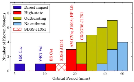
The period distribution of AM CVn stars is shown in Figure1, and their periods are summarised in TableA1. Ow-ing to the high rate of period change at short periods, high-state AM CVn stars are expected to be in the minority ( De-loye et al. 2007). Only 5 disc-accreting, high-state AM CVn-type systems are currently known (including ES Cet). There is a large gap at short periods between ES Cet (10.3 minutes) and AM CVn itself (17.1 minutes).

Although AM CVn stars often show variability on a multitude of timescales (Fontaine et al. 2011;Kupfer et al. 2015), there are three characteristic timescales that have physical motivation (Skillman et al. 1999). Firstly, the or-bital period can be measured spectroscopically, and in some systems has a photometric equivalent as well (eg. Copper-wheat et al. 2011b). Secondly, if the disc of the AM CVn is eccentric (as is possible due to their mass ratios,Whitehurst 1988), the disc will precess under the tidal field of the donor. This precession period is occasionally visible in either spec-troscopy or photometry of AM CVn systems (eg.Patterson et al. 1993;Skillman et al. 1999). Thirdly, a photometric sig-nal at a period known as the ‘superhump’ period is visible in many AM CVn stars, especially in high-state systems or systems in outburst. This signal originates from a tidal inter-action between the disc and the donor star, and is found at the beat frequency between the orbital and disc precession periods (Patterson et al. 1993)

fsh= forb±fprec. (1)

A superhump period which is longer than the orbital pe-riod (‘₋’ in Equation1) indicates that the disc precession is apsidal (precession within the plane of the system). A superhump period which is shorter than the orbital period indicates that the disc precession is nodal (precession of the

5 10 20 40 60

Orbital Period (mins)

0 2 4 6 8

Number

of

Known

Systems

HM

Cnc

V407

V

ul

ES

Cet

SDSS

J1351 AM

CVn;

J1908;

HP

Lib

CXOGBS

J1751

Direct impact High-state Outbursting No outburst SDSS J1351

Figure 1. The logarithmic orbital period distribution of all AM CVns with published orbital periods, highlighting the orbital period of J1351 presented in this work. High-state and direct-impact binaries are labelled. The periods of these systems, along with references, are given in TableA1.

axis of rotation of a tilted disc). In both AM CVn bina-ries and SU UMa binabina-ries (a class of CVs which exhibit the same phenonemon), apsidal precession is found to be more common. The orbital period and superhump period are sim-ilar in length (generally within a few percent). Therefore, even in systems which show photometric signatures on both timescales, photometry over a long baseline is often required to separate the two signals (eg.Armstrong et al. 2012).

Space-based photometry can be a powerful tool for re-solving similar signals by providing continuous, long-baseline coverage of a target.Fontaine et al.(2011) reported the dis-covery of SDSS J1908+3940, a high-state AM CVn found in theKepler field. The full 1052-dayKepler lightcurve on that system was presented inKupfer et al.(2015), in which the long baseline allowed for exquisite constraints on the system’s periods and their long-term phase evolution. In this paper, we present the discovery of SDSS J135154.46-064309.0 (henceforth J1351), a high-state AM CVn discov-ered in long-cadenceK2 photometry from Campaign 6.

In Section2, we describe the originalK2 observations as well as follow-up observations undertaken to characterise the system. In Section3, we present the data obtained dur-ing these observations. Finally in Section4, we justify the AM CVn classification and describe our interpretation of these data in the context of that classification.

2 OBSERVATIONS

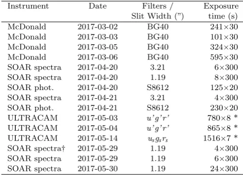
A summary of the observations obtained for this work is given in Table1.

2.1 K2 Photometry

Table 1.A summary of the follow-up observations presented in this work. Spectra are in the wavelength range 3600–5200 ˚A ex-cept where marked with a†.

Instrument Date Filters /

Slit Width (”)

Exposure time (s)

McDonald 2017-03-02 BG40 241×30

McDonald 2017-03-03 BG40 101×30

McDonald 2017-03-05 BG40 324×30

McDonald 2017-03-06 BG40 595×30

SOAR spectra 2017-04-20 3.21 6×300

SOAR spectra 2017-04-20 1.19 8×300

SOAR phot. 2017-04-20 S8612 125_×20

SOAR spectra 2017-04-21 3.21 4×300

SOAR phot. 2017-04-21 S8612 230×20

ULTRACAM 2017-05-03 u’ g’ r’ 780×8 *

ULTRACAM 2017-05-04 u’ g’ r’ 865×8 *

ULTRACAM 2017-05-14 usgsrs 1516×7 *

SOAR spectra† 2017-05-29 1.19 4×300

SOAR spectra 2017-05-29 1.19 6×300

SOAR spectra 2017-05-30 1.19 24×300

* Exposure times foru’ anduswere increased by a factor of 3 to compensate for the lower sensitivity in that band.

†Wavelength range 5200–6700˚A.

We examined several different pipeline extractions of the K2 photometry, and settled on a final light curve pro-duced from the Pre-search Data Conditioning pipeline from the Kepler Guest Observer office (Van Cleve et al. 2016), which uses a 4-pixel fixed aperture.

2.2 McDonald/ProEM Photometry

The appearance of periodic variability in the K2 data of J1351 motivated the collection of follow-up data to charac-terise the system. We obtained time series photometry on J1351 on 2017 March 2, 3, 5, and 6 with a frame-transfer Princeton Instruments ProEM camera on the 2.1m Otto Struve Telescope at McDonald Observatory. Observations were made through a broad (3300−6000˚A) BG40 filter to reduce sky noise, and each exposure was 30 s long. We dark-and flat-corrected each frame with stdark-andard IRAF tasks, us-ing calibration data from the start of each observus-ing night. We measured circular aperture photometry for the target and two bright comparison stars in the field using the IRAF scriptCCD_HSP (Kanaan et al. 2002). We correct for trans-parency variations and obtain our final relative light curves by dividing the target flux by the weighted mean of the com-parison star fluxes.

2.3 SOAR/Goodman Spectroscopy

We obtained optical spectra in April and May 2017 using the 4.1-m Southern Astrophysical Research (SOAR) telescope at Cerro Pach´on in Chile. We used the high-throughput Goodman spectrograph (Clemens et al. 2004) with a 930 line mm−1 grating, with two different grating/camera angle setups that cover roughly 3600₋5200˚A and 5200₋6700˚A. In April 2017 we used both a 3.2100and 1.1900slit, covering a wavelength range of3600₋5200˚A. In May 2017, the 1.1900 slit was used in both wavelength ranges. The 1.1900spectra have a resolution of 2.4 ˚A.

All spectra were reduced using the software packages

pamelaand molly. The data obtained with the 1.1900 slit

were wavelength calibrated using iron arc lamp spectra that were recorded before and after the spectra, as well as being interspersed every 30 minutes on 30 May. The 3.2100 spec-tra were wavelength-calibrated using a master arc that was recorded prior to observing, but these spectra suffer from large wavelength drifts and are not reliable for precision ve-locities.

The April spectra were flux-calibrated using the stan-dard star LTT 3218, observed through a 3.2100slit. No flux standard was observed in May due to poor weather condi-tions. Instead, these spectra were flux-calibrated by compar-ison with the April data. A third-order spline was fitted to averaged spectra from each night, and uncalibrated spectra were multiplied throughout by the ratio of those splines.

2.4 SOAR/Goodman Photometry

We also followed up J1351 with time-series photometry us-ing SOAR/Goodman over two consecutive nights in April 2017. Our observations were obtained through a blue, broad-bandpass, red-cutoff S8612 filter. All exposures were 20 s, with roughly 2.1 s dead time for readouts. We bias- and flat-corrected each frame with standard IRAF tasks, and per-formed circular aperture photometry.

2.5 NTT/ULTRACAM Photometry

Further follow-up photometry was obtained using ULTRA-CAM, a high-speed, triple-band photometer which uses frame-transfer CCDs to reduce the readout time overhead to negligible amounts (25 ms; seeDhillon et al. 2007, for a full description of the instrument). For these observations ULTRACAM was mounted on the 3.5 m New Technology Telescope (NTT) at the La Silla Observatory in Chile. J1351 was observed in May 2017 using Sloanu’ g’ r’filters for two nights and the custom ‘Super-SDSS’ filters usgsrs for the third night. The latter set of filters are designed to cover the same wavelength range as u’ g’ r’ filters with a higher throughput.

The ULTRACAM data were reduced using the stan-dard ULTRACAM pipeline. Images were bias- and dark-subtracted and were divided throughout by a flat field taken during the run. Due to poor weather conditions no flat field was available using theusgsrsfilters, sou’ g’ r’flats were used instead. The target was flux-calibrated using a nearby, non-variable SDSS comparison star (SDSS J135203.48-064405.1,

mu’=17.26,mg’=15.64,mr’=15.11, all error bars 0.01 mag

or less). As no flux standards exist for theusgsrsfilters the absolute flux calibration of data from those filters may not be reliable, but these data are only used for timing pur-poses. Transparency changes due to clouds or atmospheric thickness were removed using the same comparison star.

3 ANALYSIS

3.1 Spectroscopy

4000

4500

5000

5500

6000

6500

Wavelength ( ˚A)

0

.

8

1

.

0

1

.

2

1

.

4

1

.

6

1

.

8

F

(normalised)

He II

He I H I

He II

He II

He I

He II

H I

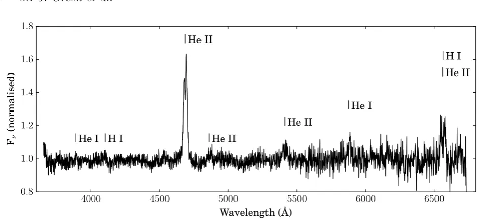
Figure 2.SOAR spectrum of J1351, showing strong, double-peaked HeII emission at 4686 ˚A and almost no emission or absorption of other elements. This spectrum is the average of 38 spectra in the 3000-5200 ˚A range (all of those with a slit width of 1.3”), and 4 spectra in the 5200-6700 ˚A range. The spectrum in the 5200-6700 ˚A range has been rebinned by a factor of 2 for visualisation purposes. The spectrum has been normalised by dividing by the continuum, which increases the apparent strength of lines at longer wavelengths where the continuum is weaker.

−4000 0 4000

0.4 0.6 0.8 1.0 1.2 1.4 1.6

Fν

(normalised)

He II

−4000 0 4000

Hα

Velocity (km/s)

Figure 3.Emission lines of J1351 at 4686 ˚A (above) and 6560 ˚A (below, offset vertically by -0.3), in both cases converted to ve-locity space. In the left panel, the 6560 ˚A line was converted as-suming it is a He II line with a central wavelength of 6560.10 ˚A. In the right panel, it is assumed to be the Hαline with a central wavelength of 6562.72 ˚A. The red line shows a double Gaussian fit to the 6560 ˚A line, described in Section3.1. In both cases this line appears to be slightly blue-shifted relative to the 4686 ˚A line, but the discrepancy is more significant when the line is treated as Hα.

and 6560 ˚A, corresponding to the Pickering series, though the latter of these occurs at a similar wavelength to Hα. Weak He I emission lines are seen at 3889 ˚A and 5876 ˚A. A weak feature is also seen at 4102 ˚A which may correspond to hydrogen, but is difficult to confirm at this S/N.

The lack of significant Hβ or Hγ suggests that the feature at 6560 ˚A can be attributed to He II rather than Hα. The strength of the 6560 ˚A line is comparable to the strengths of the other lines in the Pickering series. In order to provide an independent test of this identification, we con-verted that region of the spectrum to velocity space twice. In the first conversion we used a central wavelength

corre-0.0 0.5 1.0 1.5 2.0

BMJD (TDB) - 0

−200 −150 −100 −50 0 50 100 150 200

Radial

V

elocity

(km

s

−

1)

Figure 4.RV data for J1351, phase-folded on a frequency of 91.7 day−1_{. This figure includes RV measurements from all 38}

spectra that were observed with a 1.31” slit and which include the 4686 ˚A line.

sponding to that of the He II line, and in the second to that of Hα. These conversions can be compared to the velocity of the He II 4686 ˚A to identify the closest match (Figure3). By fitting the line profiles with a double Gaussian shape (first converged on the He II 4686 ˚A line to constrain its parameters), we measured velocity shifts of ₋20_±70km/s for the He II case and₋140_±70km/s for the Hα case. This gives a marginal preference for He II, in accordance with our identification.

80 85 90 95 100 105 110 0.0

0.2 0.4 0.6 0.8 1.0 1.2 1.4

Amplitude

(%) K2

80 85 90 95 100 105 110

0 1 2 3 4 5 6 7

Amplitude

(%) HighSpeed 2017 Mar 05+06 BG40_{2017 May 03+04 g’}

80 85 90 95 100 105 110

0 20 40 60 80 100 120

Amplitude

(km/s)

RVs 2017 May

2017 May 30

80 85 90 95 100 105 110

Frequency (cycles day−1₎

0 2 4 6 8 10

Amplitude

(%) EW 2017 May

Figure 5.Lomb-Scargle periodograms of various datasets over-plotted for comparison. Red and yellow dashed lines show the proposed superhump and orbital periods, with circle and dia-mond markers in the second panel indicating the predicted ampli-tudes of those signals (calculated from theK2 signals according to Equation2, and assuming the amplitude of variation is con-stant for all wavelengths of light). The purple dashed line shows the harmonic of theK2 Nyquist frequency. The strongK2 peaks in the top panel are Nyquist bounces of the 2.1660(2) peak, which clearly have no corresponding peak in the high-cadence data.

implemented in the Python package astropy) combining consecutive nights of RV data splits this peak into multi-ple aliases (Figure5).

The 4686 ˚A line has an equivalent width of −16.6±

0.2˚A. There is some periodicity in the equivalent widths measured (Figure 5). However, its period is closer to the observed photometric period (next section) than the spec-troscopic RV period, and we suggest that this results from variations in the continuum rather than in the spectral line.

3.2 K2 Photometry

The Nyquist frequency of the K2 data is 24.47 day−1. For any signal with a frequency higher than the Nyquist fre-quency of the data, there are several systematic effects which must be taken into account (Bell et al. 2017b). Firstly, any super-Nyquist frequency will be under-sampled, and there-fore there will be a sub-Nyquist frequency from which it is in-distinguishable. This results in the effect known as ‘Nyquist

0 20 40 60 80 100 120

Frequency (cycles day−1₎

0.0 0.5 1.0 1.5 2.0 2.5 3.0 3.5 4.0

Amplitude

(%)

Figure 6.Lomb-Scargle periodogram of K2 data, showing a clear peak at 2.162(4) day−1 along with its higher-frequency Nyquist bounces. The Nyquist frequency of 24.47 day−1and its harmonics are shown by dashed purple lines. Red circles and yellow diamonds show the predicted frequencies and intrinsic amplitudes of super-Nyquist signals that may correspond to the 8.506(2) day−1 _and

6.339(2) day−1 _{K2 signals, with frequencies reflected about the}

Nyquist frequency and its harmonics, and amplitudes corrected according to Equation2.

0.0 0.5 1.0 1.5 2.0

Phase

−0.06 −0.04 −0.02 0.00 0.02 0.04 0.06

Relative

Amplitude

Figure 7. Phase-fold of the K2 data on a frequency of 2.162 day−1_{. Individual data are shown as black circles, with red}

circles representing 20 bins of the data. Although the individual data show considerable scatter, the binned data is well-described by a sinusoid (red dashed line).

bounces’, in which a periodogram will show each signal sev-eral times, reflected off each harmonic of the Nyquist fre-quency. Secondly, as the exposure time of the observation is significant compared to the period of any super-Nyquist variability, the signal will be smeared. This causes a reduc-tion in the measured amplitude. For a sinusoidal signal, this reduction in amplitude can be described by

Ameasured/Aintrinsic=sinc(πtexp/P) (2)

wherePis the period of the signal,texpis the exposure time,

and sinc(x) =sin(x)/x.

0 10 20 30 40 50 60 70

Days (BMJD - 57216.96)

1.6 1.8 2.0 2.2 2.4 2.6 2.8

F

requency

(da

y

−

1)

0.30 0.45 0.60 0.75 0.90 1.05 1.20 1.35 1.50

Amplitude

(%)

Figure 8. A running periodogram of the K2 data, created by separating theK2 data into 20 non-overlapping subsections and calculating periodograms of each. We find no significant variation in the frequency of the 2.1660(2) day−1_signal.

Table 2.The sub-Nyquist peaks in a periodogram ofK2 data. Frequencies and amplitudes were found by fitting sine waves to theK2 data.

Frequency (day−1_{) Measured Amplitude (%)}

2.1660(2) 1.20(4)

8.506(2) 0.21(5)

6.339(2) 0.26(7)

far the highest measured amplitudes of all signals present (Figure 6). A phase fold of the K2 photometry on the 2.1660(2) day−1 frequency shows that the signal is well-approximated by a sinusoid (Figure 7). Given the smear-ing effect described in Equation 2, the intrinsic amplitude of this variability would have to be large (>25%) if the intrinsic frequency were super-Nyquist. To investigate the constancy of this signal, we separated the K2 data into 20 non-overlapping sections and produced a periodogram of each section (Figure8). When compared with a constant frequency the frequencies measured from these subdivisions haveχ2=24.1, and the phase offsets haveχ2=16.2, both for 19 degrees of freedom. We therefore do not find any evidence that the frequency of this signal is variable.

Two lower-amplitude signals are also visible in the pe-riodogram (Figure6). We summarise their sub-Nyquist fre-quencies in Table2. If these signals are super-Nyquist, their intrinsic amplitudes can be predicted by Equation 2 (see Figure6).

These three signals obey Equation1to within1σ. The same is true for any Nyquist bounce of the 8.506(2) day−1 and 6.339(2) day−1 _{signals, provided that both are} sub-ject to the same number of Nyquist bounces and that the 2.1660(2) day−1_{signal is sub-Nyquist. In order to determine} the number of Nyquist bounces which these signals are sub-ject to, it is necessary to examine higher-cadence photometry of the system.

3.3 High-cadence photometry

The McDonald, SOAR, and ULTRACAM photometric data are shown in Figure9. The mean AB magnitudes and scat-ters across both ULTRACAM nights withu’ g’ r’ filters are

mu’=18.46±0.08,mg’=18.60±0.07, andmr’=18.95±0.07,

where the quoted error bars are one standard deviation of the data so as to include the intrinsic variability of the sys-tem. The data show variability with a period of

approxi-mately 15 minutes (_≈90 day−1_{) and an amplitude on the} or-der of 4–6%, with changes to the lightcurve shape between one cycle and the next. Figure5 shows Lomb-Scargle pe-riodograms produced from the ULTRACAM and McDon-ald data, each using data from two consecutive nights. Sev-eral nights also show long-term trends in brightness (on timescales longer than the observing window of these data), which may correspond to the 2.1660(2) day−1signal, but are more likely to be due to changes in airmass as has previously been observed with the same McDonald setup (Bell et al. 2017a).

These data can be used to select between the Nyquist bounces of the signals in the K2 data discussed in Sec-tion3.2. All Nyquist reflections of the 2.1660(2) day−1_peak in theK2 data can be easily ruled out. Given the smearing effect described in Equation2, the intrinsic amplitude of this signal would have to be>25% if it were super-Nyquist, and such a signal is clearly not present in the short cadence pho-tometry. It is therefore most likely that the true frequency detected by K2 is 2.1660(2) day−1, corresponding to a pe-riod of664.82_±0.06min. This period is not measurable in the ground-based data due to the short observing windows of those data.

The≈90 day−1signal in the high-cadence data lies be-tween the third Nyquist reflections of the measured frequen-cies for both the 6.339(2) day−1_{and the 8.506(2) day}−1 sig-nals, which would give these signals intrinsic frequencies of 89.374(2) day−1_{and 91.541(2) day}−1_{. We therefore interpret} the variability seen in the high-cadence data as a combina-tion of both intrinsic signals. As shown in Figure5, nightly aliasing makes it nearly impossible to disentangle the two signals using single-site, ground-based data. The amplitude measured in the high-cadence data agrees well with the pre-diction made from the measured K2 amplitude by Equa-tion2. The strength of this agreement and the lack of other signals in the short-cadence photometry leads us to interpret 89.374(2) day−1 _{and 91.541(2) day}−1 _{as the true} frequen-cies of the signals found in theK2 data. Phase-folding the ULTRACAM and McDonald data on these two frequencies gives very similar, sawtooth-shaped lightcurves (Figure10). The amplitudes of the two signals are approximately equal at their fundamental frequencies. At their third har-monic (we use “third harhar-monic” to refer to 3f0, where f0 is the fundamental harmonic) the higher frequency signal of the two has a higher amplitude than the shorter period signal.

4 DISCUSSION

4.1 Classification as an AM CVn star

0

.

0

0

.

5

1

.

0

1

.

5

2

.

0

2

.

5

3

.

0

3

.

5

4

.

0

4

.

5

5

.

0

5

.

5

6

.

0

−

0

.

2

−

0

.

1

0

.

0

0

.

1

McDonald 2017 Mar 06

0

.

0

0

.

5

1

.

0

1

.

5

2

.

0

2

.

5

−

0

.

2

−

0

.

1

0

.

0

0

.

1

SOAR 2017 Apr 21

0

.

0

0

.

5

1

.

0

1

.

5

2

.

0

2

.

5

−

0

.

2

−

0

.

1

0

.

0

0

.

1

SOAR 2017 Apr 20

0

.

0

0

.

5

1

.

0

1

.

5

2

.

0

2

.

5

−

0

.

2

−

0

.

1

0

.

0

0

.

1

McDonald 2017 Mar 05

0

.

0

0

.

5

1

.

0

1

.

5

2

.

0

2

.

5

−

0

.

2

−

0

.

1

0

.

0

0

.

1

McDonald 2017 Mar 03

0

.

0

0

.

5

1

.

0

1

.

5

2

.

0

2

.

5

−

0

.

2

−

0

.

1

0

.

0

0

.

1

McDonald 2017 Mar 02

0

.

0

0

.

5

1

.

0

1

.

5

2

.

0

2

.

5

3

.

0

−

0

.

8

−

0

.

6

−

0

.

4

−

0

.

2

0

.

0

0

.

2

0

.

4

0

.

6

ULTRACAM 2017 May 14

0

.

0

0

.

5

1

.

0

1

.

5

2

.

0

2

.

5

3

.

0

−

0

.

8

−

0

.

6

−

0

.

4

−

0

.

2

0

.

0

0

.

2

0

.

4

0

.

6

ULTRACAM 2017 May 04

0

.

0

0

.

5

1

.

0

1

.

5

2

.

0

2

.

5

3

.

0

−

0

.

8

−

0

.

6

−

0

.

4

−

0

.

2

0

.

0

0

.

2

0

.

4

0

.

6

ULTRACAM 2017 May 03

Relative

Flux

Time (hours)

Figure 9.All short-cadence photometry of J1351 obtained for this project. For the ULTRACAM data, ther’/rs-band andu’/us-band data have been offset by +0.4 and -0.4 respectively. Most observing runs clearly show sawtooth-shaped variability on a frequency of around 90 day−1_{. On some nights (see April 21) this signal changes significantly in shape and amplitude between cycles. Some runs (see}

March 06 and May 03) also show evidence for longer-term variability in brightness. The quality of data from March 02, March 03 and May 14 data was affected by poor conditions.

AM CVn-type binary to accrete via an accretion disc (see Figure1).

He II emission lines are also seen in HM Cnc and ES Cet, which are both at shorter orbital periods than J1351. In ES Cet the 4686 ˚A line is particularly strong with an equiva-lent width of₋80˚A (Espaillat et al. 2005, cf.₋16.6˚A for the same line in J1351). High-state AM CVns at longer periods than J1351 all show absorption lines rather than emission. It may therefore be the case that J1351 lies close to a

0.0 0.5 1.0 1.5 2.0 −0.20

−0.15 −0.10 −0.05 0.00 0.05 0.10 0.15 0.20

Relative

Amplitude

0.0 0.5 1.0 1.5 2.0

Phase

−0.20 −0.15 −0.10 −0.05 0.00 0.05 0.10 0.15 0.20

Relative

Amplitude

Figure 10. Phase folds of all g’ ULTRACAM photometry and BG40 McDonald photometry of J1351 on frequencies of 91.541(2) day−1 _{(top panel) and 89.374(2) day}−1 _{(bottom panel).}

The red lines show mean values calculated from a series of 20 phase bins. Both signals have a sawtooth shape, with a steep rise and a gentle decline, which may be the result of beating between the two signals.

4.2 The Nature of the Photometric Periods

In comparison with other AM CVns that have been ob-served over a long baseline (eg.Skillman et al. 1999;Kupfer et al. 2015), J1351 is unusually well-behaved photometri-cally. Only three photometric periods have been identified in J1351, all of which appear to be stable over the baseline of observations. These three signals are in good agreement with Equation 1. In this section we will use the data presented thus far to establish the physical origin of these signals.

The high frequency signals correspond to periods of 15.7306(3) minutes and 16.1121(4) minutes. These periods are comparable to the spectroscopic orbital period of15.65_± 0.12minutes. The likely interpretation is therefore that one signal is at the orbital period and the other the superhump period, an interpretation backed up by the agreement of these periods with Equation 1. The 15.7 minute signal is clearly in closer agreement with the spectroscopic orbital period.The 16.11 minute signal disagrees with the spectro-scopic period at the 3.9σ level, and is most likely to be the superhump period. This interpretation fits with the pattern that orbital periods are generally shorter than superhump periods. We therefore consider this the most probable

inter-Table 3.Summary of properties of J1351, as derived from the

K2 data. Periods are given in minutes.

Property Value

Orbital period 15.7306±0.0003

Superhump period 16.1121±0.0004

Disc precession period 664.82±0.06

Superhump excessε 0.02425±0.00003

Estimated mass ratioq 0.111±0.005

pretation of the signals, suggesting that the disc is undergo-ing apsidal precession. However, we note that the possibility that they may be the other way around has not been con-clusively ruled out. The χ2 values of sinusoidal fits to the RV data are 56.2 and 86.0 with 35 degrees of freedom.

This interpretation means that it is the orbital period which has a strong third harmonic (3f0). This may be related to the 3:1 resonance between the orbital period of the binary and the orbital period of a region of the disc, which is crucial to the mechanism by which the disc is driven to be eccentric. The agreement with Equation1implies that the low fre-quency signal of 2.1660(2) day−1, corresponding to a period of664.82_±0.06min, originates from the precession period of the eccentric disc. The period is of the correct order for this interpretation; variability attributed to disc precession has been detected at a similar period (13.38 hours) in AM CVn itself (Patterson et al. 1993;Skillman et al. 1999). The ap-parent stability of this signal throughout theK2observation period is somewhat surprising given the variable nature of accretion discs. It suggests that the radius of the accretion disc remains approximately constant throughout the period of observation.

4.3 Mass Ratio

Taking the measurements of the orbital and superhump fre-quencies determined in Section4.2, we can estimate the mass ratio,q=M2/M1, of the binary from the empirical relation with superhump excess (Knigge 2006)

q(ε) = (0.114±0.005) + (3.97±0.41)×(ε−0.025) (3) whereε= (Psh−Porb)/Porbis the superhump excess. This

re-lation gives similar results to that ofPatterson et al.(2005), but with the inclusion of uncertainties on the fit parame-ters. When applied to J1351 these uncertainties dominate due to the small uncertainty onε. We emphasise that this relation was derived for hydrogen-dominated CVs, and has not yet been well tested for AM CVns (see eg.Roelofs et al. 2006). With this caveat, we find ε=0.02425(3)which gives an estimate ofq=0.111_±0.005.

evolution-Table 4.A summary of the AM CVn mass ratios used for Figure11. Whereqwas derived by the superhump method, we recalculate it using Equation3for the sake of consistency.

Designation ε q M2 (M) Method Reference

SDSSJ1351-0643 0.024±0.000 0.111±0.005 – Superhumps 1

AM CVna _{0.022±0.000 0.180±0.010 0.125±0.012 Spectroscopy 2}

HP Lib 0.015±0.000 0.074±0.007 – Superhumps 3

CXOGBS J1751-2940 0.014±0.001 0.070±0.007 – Superhumps 4

CR Boo 0.011±0.000 0.058±0.008 – Superhumps 3

KL Dra 0.019±0.000 0.092±0.006 – Superhumps 5,6

V803 Cen 0.011±0.003 0.058±0.014 – Superhumps 3

YZ LMib 0.009±0.000 0.041±0.002 0.035±0.003 Eclipses 7

CP Eri 0.009±0.001 0.051±0.008 – Superhumps 8

SDSSJ1240-0159 – 0.039±0.010 – Spectroscopy 9

SDSSJ0129+3842 0.009±0.005 0.051±0.023 – Superhumps 10

GP Com – 0.020±0.003 – Spectroscopy 11

SDSSJ0902+3819 0.005±0.002 0.033±0.012 – Superhumps 12

Gaia14aae – 0.029±0.002 0.025±0.001 Eclipses 13

V396 Hya – 0.014±0.004 – Spectroscopy 14

References: [1] Green in prep; [2] Roelofs et al. (2006); [3]Roelofs et al. (2007d); [4]Wevers et al.(2016); [5]Wood et al. (2002); [6]Ramsay et al.(2010); [7]Copperwheat et al.(2011a); [8]Armstrong et al.(2012); [9]Roelofs et al.(2005); [10]Kupfer et al.(2013); [11]Marsh(1999); [12]Kato et al.(2014); [13]Green et al.(2018); [14]Kupfer et al.(2016).

a _{The tabulatedqfor AM CVn itself is derived from spectroscopy; its superhump excess gives}

q=0.101±0.005by Equation3

b _{The tabulatedq for YZ LMi is derived from eclipse photometry; its superhump excess gives}

q=0.049±0.008by Equation3

−2.2 −2.0 −1.8 −1.6 −1.4 −1.2 −1.0 −0.8 log (M2/ M)

−1.7

−1.6

−1.5

−1.4

−1.3

−1.2

−1.1

log

(R2 /R

)

J1351 AM CVn

HP Lib CXOGBS J1751

J1351 (this work) Superhump-derivedq

Eclipse-derivedq

Spectroscopy-derivedq

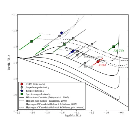
White dwarf models (Deloye et al. 2007) Helium-star models (Yungelson, 2008) Hydrogen-CV models (Goliasch & Nelson, 2015) Hydrogen-CV models (Goliasch & Nelson, priv. comm.)

Figure 11. Measured donor masses or mass ratios for a sam-ple of AM CVns, compared to predictedM–R tracks for donors in AM CVns descended from three proposed formation channels. Error bars are diagonal because of the strong constraint on mean density which comes from orbital period (Faulkner et al. 1972). The thick black line shows theM–R relation for a zero-entropy white dwarf. For systems where M1 is not known, a value of 0.7±0.1has been assumed.

ary channels which may contribute to the AM CVn popula-tion. A brief overview of these channels is as follows. In the white dwarf donor channel (Paczy´nski 1967; Deloye et al. 2007), the system evolves from a detached binary consisting of two white dwarfs. These white dwarfs inspiral due to grav-itational wave radiation until they are close enough to

be-gin mass transfer, at orbital periods of around 5–10 minutes. The white dwarf which becomes the donor may not be com-pletely degenerate. The helium star donor channel (Savonije et al. 1986;Iben & Tutukov 1987;Yungelson 2008) is sim-ilar, but in this case the progenitor system consists of one white dwarf and one core helium-burning star, the atmo-sphere of which has been stripped. In a system descended through this channel, the additional thermal support within the donor will give it a larger radius for a given mass. In the evolved CV channel (Tutukov et al. 1985;Podsiadlowski et al. 2003; Goliasch & Nelson 2015), the AM CVn is de-scended from a CV with an evolved donor. As the atmo-sphere of the donor is stripped away and its helium core is revealed, the transferred matter becomes helium-dominated. This channel predominantly forms AM CVns with long or-bital periods, and is thought to make only a negligible con-tribution to the population of AM CVns with orbital periods of less than 30 minutes (Nelemans et al. 2004;Goliasch & Nelson 2015).

From Figure11, the population as a whole appears to include only donors with a significant amount of thermal support. Given the tracks shown here, this seems to favour the helium star donor channel. This is not conclusive, how-ever: it may also be the case that the effect of irradiation of the donor star has been underestimated. It is also worth not-ing that mass ratios derived by the superhump relation may yet have an unknown bias in helium-dominated systems.

4.4 Distance and Space Density

After SDSS 1908+3940 (Fontaine et al. 2011), J1351 is the second AM CVn to be discovered in the footprints ofKepler

andK2. Given the rarity of AM CVns, this is worthy of note. A survey of AM CVns in 11663 square degrees of SDSS DR7 that was complete to a magnitude g’<19 included only 4 AM CVns within that magnitude limit (Carter et al. 2013, though note the total number of AM CVns discovered by the survey was larger). Based on this,Carter et al.(2013) esti-mated an AM CVn space density of(5±3)×10−7pc−3_{. Both} high-state systems found byKeplerandK2 are also within the g’<19 limit. Scaling the population found by Carter et al.(2013) by the ratio of that area to the totalKepler+K2

area up to and including Campaign 6 (_≈750 square de-grees) we would expect 0.25 AM CVns with g’<19 in the

Kepler+K2 footprint.Kepler andK2 have therefore found more AM CVns than would be expected, but given the small numbers involved and the large uncertainty on the space density, the discrepancy is unlikely to be significant.

Also surprising is the coincidence that both these sys-tems are high-state binaries. Including J1351, the six known high-state systems comprise only_∼12per cent of the known AM CVn population. However, the sample of all known sys-tems includes a selection bias toward outbursting syssys-tems due to transient surveys (eg.Levitan et al. 2013). If we de-fine a sample including only systems with magnitudes<19

(the magnitude limit used byGentile Fusillo et al. 2015, who selected this object as a candidate white dwarf), using qui-escent magnitudes for outbursting systems, the bias towards outbursting systems is reduced. High-state systems become ∼35–40 per cent of the sample, and finding two high-state systems then becomes somewhat more probable. Note that high-state systems are expected to make up.2per cent of the AM CVn population (Roelofs et al. 2007b), but this is countered in a magnitude-limited sample by their brighter absolute magnitudes.

An estimate of the distance to J1351 can be made from the predicted absolute magnitudes for disc-dominated AM CVns calculated by Nelemans et al. (2004). For an AM CVn with this orbital period, the predicted absolute magnitude would be _≈6–8. By comparison with our ap-parent magnitude we estimate a distance of 130–330 pc. This prediction assumes an AM CVn descended from a dou-ble white dwarf; if the donor of the system is instead de-scended from a semi-degenerate helium star, the mass trans-fer rate would be greater and hence the magnitude would be brighter, giving a larger distance. A reliable distance es-timate should be given byGaia (Gaia Collaboration et al. 2016) in the near future.

5 CONCLUSIONS

We have presented the discovery of J1351, a system with a spectroscopic period of15.65±0.12 minutes that was dis-covered using K2 data. The spectrum, orbital period, and lightcurve of this object are consistent with a classification as an AM CVn-type binary. This makes J1351 one of only a small number of known disc-accreting high-state AM CVn-type systems, and the second discovered usingKeplerorK2

photometry.

J1351 has several visible photometric periods, including a disc precession period at 664.82_±0.06minutes, a signal at 15.7306±0.0003minutes which is in agreement with its orbital period, and a signal at16.1121_±0.0004minutes which we identify as the superhump period. Using the empirical relation of Knigge (2006), we can estimate the mass ratio of the binary asq=M2/M1=0.111±0.005. This mass ratio is presented with the caveat that the relationship between superhump excess and mass ratio may not be reliable for helium-dominated binaries.

As a short-period AM CVn, J1351 is likely to be a bright emitter of low-frequency gravitational waves. Further study may provide the mass estimates required to quantify its emission. The presence of a photometric signature of the or-bital period provides an exciting opportunity to track the pe-riod evolution of the system over the next few years, provid-ing a constraint on the system component masses. However, the alignment of this period with a nightly alias of the super-hump period means such efforts will likely require multi-site observations if performed from the ground. The system has been re-observed by K2 in Campaign 17 in short-cadence (58.8 s) mode, allowing an opportunity to revisit this analy-sis and providing a longer baseline with which to constrain the period evolution.

This work highlights the fact that AM CVns have pho-tometric variability on both short and long timescales. Sus-tained, high-speed photometry can yield a great deal of in-formation on the nature of the system.

ACKNOWLEDGEMENTS

The authors are grateful to Thomas Kupfer and Gavin Ram-say for their help in assembling Table A1, as well as to Mukremin Kilic, whose Guest Observer program GO6003 ensured the discovery of J1351.

MJG acknowledges funding from an STFC studentship via grant ST/N504506/1. Support for this work was pro-vided by NASA through Hubble Fellowship grant #HST-HF2-51357.001-A, awarded by the Space Telescope Science Institute, which is operated by the Association of Universi-ties for Research in Astronomy, Incorporated, under NASA contract NAS5-26555. TRM, DTHS and EB acknowledge STFC via grants ST/L000733/1 and ST/P000495/1. KJB acknowledges support from NSF grant AST-1312983. VSD, SPL, and ULTRACAM are funded by STFC via consol-idated grant ST/J001589. The research leading to these results has received funding from the European Research Council under the European Union’s Seventh Framework Programme (FP/2007-2013) / ERC Grant Agreement n. 320964 (WDTracer).

Michigan State University (MSU). It is also based on obser-vations collected at the European Organisation for Astro-nomical Research in the Southern Hemisphere.

This publication made use of the packages pamela,

molly,numpy,matplotlib,astropy, andscipy.

REFERENCES

Armstrong E., Patterson J., Kemp J., 2012,Monthly Notices of the Royal Astronomical Society, 421, 2310

Bell K. J., et al., 2017a,The Astrophysical Journal, 835, 180 Bell K. J., Hermes J. J., Vanderbosch Z., Montgomery M. H.,

Winget D. E., Dennihy E., Fuchs J. T., Tremblay P.-E., 2017b,

The Astrophysical Journal, 851, 24

Breedt E., 2015,Proceedings of The Golden Age of Cataclysmic Variables and Related Objects - III (Golden2015), p. 25 Campbell H. C., et al., 2015, Monthly Notices of the Royal

As-tronomical Society, 452, 1060

Cannizzo J. K., Nelemans G., 2015,The Astrophysical Journal, 803, 19

Carter P. J., et al., 2013, Monthly Notices of the Royal Astro-nomical Society, 429, 2143

Carter P. J., Steeghs D., Marsh T. R., Kupfer T., Copperwheat C. M., Groot P. J., Nelemans G., 2014a,Monthly Notices of the Royal Astronomical Society, 437, 2894

Carter P. J., et al., 2014b,Monthly Notices of the Royal Astro-nomical Society, 439, 2848

Clemens J. C., Crain J. A., Anderson R., 2004, in Moor-wood A. F. M., Iye M., eds, Proc. SPIEVol. 5492, Ground-based Instrumentation for Astronomy. pp 331–340,

doi:10.1117/12.550069

Copperwheat C. M., et al., 2011a,Monthly Notices of the Royal Astronomical Society, 410, 1113

Copperwheat C. M., et al., 2011b,Monthly Notices of the Royal Astronomical Society, 413, 3068

Cropper M., Harrop-Allin M. K., Mason K. O., Mittaz J. P. D., Potter S. B., Ramsay G., 1998,Monthly Notices of the Royal Astronomical Society, 293, L57

Deloye C. J., Taam R. E., Winisdoerffer C., Chabrier G., 2007,

Monthly Notices of the Royal Astronomical Society, 381, 525 Dhillon V. S., et al., 2007,Monthly Notices of the Royal

Astro-nomical Society, 378, 825

Espaillat C., Patterson J., Warner B., Woudt P., 2005, Publica-tions of the Astronomical Society of the Pacific, 117, 189 Faulkner J., Flannery B. P., Warner B., 1972,The Astrophysical

Journal, 175, L79

Fontaine G., et al., 2011,The Astrophysical Journal, 726, 92 Gaia Collaboration et al., 2016,A&A,595, A1

Gentile Fusillo N. P., G¨ansicke B. T., Greiss S., 2015,MNRAS,

448, 2260

Goliasch J., Nelson L., 2015,The Astrophysical Journal, 809, 80 Green M. J., et al., 2018, MNRAS, 476, 1663

Iben I. J., Tutukov A. V., 1987,The Astrophysical Journal, 313, 727

Israel G. L., et al., 2002,Astronomy and Astrophysics, 386, L13 Ivanova N., et al., 2013,Astronomy and Astrophysics Review, 21,

59

Kanaan A., Kepler S. O., Winget D. E., 2002,Astronomy & As-trophysics, 389, 896

Kato T., et al., 2014,Publications of the Astronomical Society of Japan, 66, L7

Knigge C., 2006,Monthly Notices of the Royal Astronomical So-ciety, 373, 484

Korol V., Rossi E. M., Groot P. J., Nelemans G., Toonen S., Brown A. G. A., 2017,Monthly Notices of the Royal Astro-nomical Society, 470, 1894

Kotko I., Lasota J.-P., Dubus G., Hameury J.-M., 2012, Astron-omy & Astrophysics, 544, A13

Kupfer T., Groot P. J., Levitan D., Steeghs D., Marsh T. R., Rutten R. G. M., Nelemans G., 2013,Monthly Notices of the Royal Astronomical Society, 432, 2048

Kupfer T., et al., 2015,Monthly Notices of the Royal Astronom-ical Society, 453, 483

Kupfer T., Steeghs D., Groot P. J., Marsh T. R., Nelemans G., Roelofs G. H. A., 2016,Monthly Notices of the Royal Astro-nomical Society, 457, 1828

Levitan D., et al., 2011,The Astrophysical Journal, 739, 68 Levitan D., et al., 2013,Monthly Notices of the Royal

Astronom-ical Society, 430, 996

Levitan D., et al., 2014,The Astrophysical Journal, 785, 114 Levitan D., Groot P. J., Prince T. A., Kulkarni S. R., Laher R.,

Ofek E. O., Sesar B., Surace J., 2015,Monthly Notices of the Royal Astronomical Society, 446, 391

Lomb N. R., 1976,Astrophysics and Space Science, 39, 447 Marsh T. R., 1999,Monthly Notices of the Royal Astronomical

Society, 304, 443

Marsh T. R., Steeghs D., 2002,Monthly Notices of the Royal Astronomical Society, 331, L7

Motch C., Haberl F., Guillout P., Pakull M., Reinsch K., Krautter J., 1996, Astronomy and Astrophysics, 307, 459

Nather R. E., Robinson E. L., Stover R. J., 1981,The Astrophys-ical Journal, 244, 269

Nelemans G., Steeghs D., Groot P. J., 2001,Monthly Notices of the Royal Astronomical Society, 326, 621

Nelemans G., Yungelson L. R., Portegies Zwart S. F., 2004, Monthly Notices of the Royal Astronomical Society, 349, 181 Paczy´nski B., 1967, Acta Astronomica, 17, 287

Patterson J., Halpern J., Shambrook A., 1993,The Astrophysical Journal, 419, 803

Patterson J., et al., 1997,Publications of the Astronomical Soci-ety of the Pacific, 109, 1100

Patterson J., et al., 2005,The Publications of the Astronomical Society of the Pacific, 117, 1204

Podsiadlowski P., Han Z., Rappaport S., 2003,Monthly Notices of the Royal Astronomical Society, 340, 1214

Provencal J. L., 1994, PhD thesis, Texas University

Provencal J. L., et al., 1991, White Dwarfs, Proceedings of the 7th European Workshop, NATO Advanced Science Institutes (ASI) Series C, 336, 449

Ramsay G., et al., 2010,Monthly Notices of the Royal Astronom-ical Society, 407, 1819

Rau A., Roelofs G. H. A., Groot P. J., Marsh T. R., Nelemans G., Steeghs D., Salvato M., Kasliwal M. M., 2010,The Astro-physical Journal, 708, 456

Roelofs G. H. A., 2007, PhD thesis, University of Nijmegen Roelofs G. H. A., Groot P. J., Marsh T. R., Steeghs D., Barros

S. C. C., Nelemans G., 2005, Monthly Notices of the Royal Astronomical Society, 361, 487

Roelofs G. H. A., Groot P. J., Nelemans G., Marsh T. R., Steeghs D., 2006,Monthly Notices of the Royal Astronomical Society, 371, 1231

Roelofs G. H. A., Groot P. J., Nelemans G., Marsh T. R., Steeghs D., 2007a,Monthly Notices of the Royal Astronomical Soci-ety, 379, 176

Roelofs G. H. A., Nelemans G., Groot P. J., 2007b,Monthly No-tices of the Royal Astronomical Society, 382, 685

Roelofs G. H. A., Groot P. J., Steeghs D., Marsh T. R., Nele-mans G., 2007c,Monthly Notices of the Royal Astronomical Society, 382, 1643

Roelofs G. H. A., Groot P. J., Benedict G. F., McArthur B. E., Steeghs D., Morales-Rueda L., Marsh T. R., Nelemans G., 2007d,The Astrophysical Journal, 666, 1174

Roelofs G. H. A., Rau A., Marsh T. R., Steeghs D., Groot P. J., Nelemans G., 2010,The Astrophysical Journal, 711, L138 Ruiz M. T., Rojo P. M., Garay G., Maza J., 2001, The

Astro-physical Journal, 552, 679

Savonije G. J., de Kool M., van den Heuvel E. P. J., 1986, As-tronomy and Astrophysics, 155, 51

Scargle J. D., 1982,The Astrophysical Journal, 263, 835 Skillman D. R., Patterson J., Kemp J., Harvey D. A., Fried R. E.,

Retter A., Lipkin Y., Vanmunster T., 1999,PASP,111, 1281

Solheim J.-E., 2010,Publications of the Astronomical Society of the Pacific, 122, 1133

Steeghs D., Marsh T. R., Barros S. C. C., Nelemans G., Groot P. J., Roelofs G. H. A., Ramsay G., Cropper M., 2006,The Astrophysical Journal, 649, 382

Tutukov A. V., Fedorova A. V., Ergma E. V., Yungelson L. R., 1985, Soviet Astronomy Letters, 11, 52

Van Cleve J. E., et al., 2016,PASP,128, 075002

VanderPlas J. T., 2017, preprint, (arXiv:1703.09824)

Wevers T., et al., 2016,Monthly Notices of the Royal Astronom-ical Society: Letters, Volume 462, Issue 1, p.L106-L110, 462, L106

Whitehurst R., 1988,Monthly Notices of the Royal Astronomical Society, 232, 35

Wood M. A., Casey M. J., Garnavich P. M., Haag B., 2002,

Monthly Notices of the Royal Astronomical Society, 334, 87 Woudt P. A., Warner B., 2003, White Dwarfs: Galactic and

Cos-mologic Probes, 25th meeting of the IAU, 5 Yungelson L. R., 2008,Astronomy Letters, 34, 620

de Miguel E., Patterson J., Kemp J., Myers G., Rea R., Krajci T., Monard B., Cook L., 2018,The Astrophysical Journal, 852, 19

APPENDIX A: SUMMARY OF PUBLISHED AM CVN ORBITAL PERIODS

Around 50 AM CVn systems are currently known. 49 were included in the most recently published count (see Breedt 2015, and the references therein).

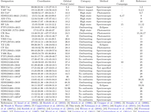
Of the known systems, we are aware of 32 which have published orbital periods (we do not include systems for which only superhump periods are known). We list these systems and their orbital periods in TableA1. We also ify whether the orbital period has been determined by spec-troscopic RVs, by eclipse timing, or by photometric mod-ulation. Those periods determined spectroscopically or by eclipse timing should be reliable. Periods which are only known through photometric modulation should be treated with caution, as such periods have been proved wrong by spectroscopic measurements in the past (eg. Roelofs et al. 2007a).

We label those systems which were visible in past K2

Campaigns and those which will be visible in the future.

This paper has been typeset from a TEX/LA_{TEX file prepared by}

Table A1.A summary of published AM CVn orbital periods. “Method” describes the method by which the orbital period was determined: either by timing of eclipses, spectroscopic RVs, or photometric variability.

Designation Coordinates Orbital

Period (min)

Category Method K2

Campaign

Reference

HM Cnc 08:06:22.84 +15:27:31.5 5.4 Direct impact Spectroscopic – 1,2

V407 Vul 19:14:26.09 +24:56:44.6 9.5 Direct impact Spectroscopic – 3,4,5

ES Ceta _{02:00:52.17 -09:24:31.7 10.3 High state Photometric – 6,7}

SDSSJ1351-0643 (J1351) 13:51:54.46 -06:43:09.0 15.7 High state Spectroscopic 6,17 8

AM CVn 12:34:54.60 +37:37:44.1 17.1 High state Spectroscopic – 9

SDSSJ1908+3940b _{19:08:17.07 +39:40:36.4 18.2 High state Spectroscopic – 10}

HP Lib 15:35:53.08 -14:13:12.2 18.4 High state Spectroscopic 15 11,12

PTF1J1919+4815 19:19:05.19 +48:15:06.2 22.5 Outbursting Eclipses – 13

CXOGBS J1751-2940 17:51:07.6 -29:40:37 22.9 High state Photometric – 14

CR Boo 13:48:55.22 +07:57:35.8 24.5 Outbursting Photometric – 15,16,17

KL Dra 19:24:38.28 +59:41:46.7 25 Outbursting Photometric – 18

V803 Cen 13:23:44.54 -41:44:29.5 26.6 Outbursting Spectroscopic – 11

PTF1J0719+4858 07:19:12.13 +48:58:34.0 26.8 Outbursting Spectroscopic – 19

YZ LMi 09:26:38.71 +36:24:02.4 28.3 Outbursting Eclipses – 20

CP Eri 03:10:32.76 -09:45:05.3 28.4 Outbursting Photometric – 21

PTF1J0943+1029 09:43:29.59 +10:29:57.6 30.4 Outbursting Spectroscopic – 22

V406 Hya 09:05:54.79 -05:36:08.6 33.8 Outbursting Spectroscopic – 23

PTF1J0435+0029 04:35:17.73 +00:29:40.7 34.3 Outbursting Spectroscopic – 22

SDSSJ1730+5545 17:30:47.59 +55:45:18.5 35.2 No outbursts Spectroscopic – 24

SDSSJ1240-0159 12:40:58.03 -01:59:19.2 37.4 Outbursting Spectroscopic 10 25

SDSSJ0129+3842 01:29:40.06 +38:42:10.5 37.6 Outbursting Spectroscopic – 26

SDSSJ1721+2733c _{17:21:02.48 +27:33:01.2 38.1 Outbursting Not specified – 27}

SDSSJ1525+3600 15:25:09.58 +36:00:54.6 44.3 Outbursting Spectroscopic – 26

SDSSJ0804+1616 08:04:49.49 +16:16:24.8 44.5 No outbursts Spectroscopic – 28

SDSSJ1411+4812d _{14:11:18.31 +48:12:57.6 46 No outbursts Spectroscopic – 29}

GP Com 13:05:42.43 +18:01:04.0 46.5 No outbursts Spectroscopic – 30,31

SDSSJ0902+3819 09:02:21.36 +38:19:41.9 48.31 Outbursting Spectroscopic – 32

Gaia14aae 16:11:33.97 +63:08:31.8 49.7 Outbursting Eclipses – 33,34

SDSSJ1208+3550 12:08:41.96 +35:50:25.2 52.96 No outbursts Spectroscopic – 26

SDSSJ1642+1934 16:42:28.08 +19:34:10.1 54.2 No outbursts Spectroscopic – 26

SDSSJ1552+3201 15:52:52.48 +32:01:50.9 56.3 No outbursts Spectroscopic – 35

SDSSJ1137+4054d _{11:37:32.32 +40:54:58.3 59.6 No outbursts Spectroscopic – 36}

V396 Hya 13:12:46.93 -23:21:31.3 65.1 No outbursts Spectroscopic – 37

References: [1]Israel et al.(2002); [2]Roelofs et al.(2010); [3] Motch et al.(1996); [4]Cropper et al.(1998); [5]Steeghs et al. (2006); [6]Woudt & Warner(2003); [7]Copperwheat et al.(2011b); [8] This work; [9]Nelemans et al.(2001); [10]Kupfer et al.(2015); [11]Roelofs et al.(2007a); [12]Roelofs et al.(2007d); [13]Levitan et al.(2014); [14]Wevers et al.(2016); [15]Provencal et al.(1991); [16]Provencal

(1994); [17] Patterson et al.(1997); [18]Wood et al. (2002); [19]Levitan et al.(2011); [20]Copperwheat et al.(2011a); [21]Armstrong et al.(2012); [22]Levitan et al.(2013); [23]Roelofs et al.(2006); [24]Carter et al.(2014a); [25]Roelofs et al.(2005); [26]Kupfer et al.

(2013); [27]Levitan et al.(2015); [28]Roelofs et al.(2009); [29]Roelofs(2007); [30]Nather et al.(1981); [31]Marsh(1999); [32]Rau et al.

(2010); [33]Campbell et al.(2015); [34]Green et al.(2018); [35]Roelofs et al.(2007c); [36]Carter et al.(2014b); [37]Ruiz et al.(2001). a _{The state of ES Cet is uncertain; it may be a direct impact (Espaillat et al. 2005) or a high state system}

b _{This system was in theKeplerfield}