warwick.ac.uk/lib-publications
Manuscript version: Author’s Accepted Manuscript
The version presented in WRAP is the author’s accepted manuscript and may differ from the
published version or Version of Record.
Persistent WRAP URL:
http://wrap.warwick.ac.uk/119433
How to cite:
Please refer to published version for the most recent bibliographic citation information.
If a published version is known of, the repository item page linked to above, will contain
details on accessing it.
Copyright and reuse:
The Warwick Research Archive Portal (WRAP) makes this work by researchers of the
University of Warwick available open access under the following conditions.
Copyright © and all moral rights to the version of the paper presented here belong to the
individual author(s) and/or other copyright owners. To the extent reasonable and
practicable the material made available in WRAP has been checked for eligibility before
being made available.
Copies of full items can be used for personal research or study, educational, or not-for-profit
purposes without prior permission or charge. Provided that the authors, title and full
bibliographic details are credited, a hyperlink and/or URL is given for the original metadata
page and the content is not changed in any way.
Publisher’s statement:
Please refer to the repository item page, publisher’s statement section, for further
information.
1
Channel Modeling for Diffusive Molecular
Communication – A Tutorial Review
Vahid Jamali,
Student Member, IEEE
, Arman Ahmadzadeh,
Student Member, IEEE
, Wayan Wicke,
Student
Member, IEEE
, Adam Noel,
Member, IEEE
, and Robert Schober,
Fellow, IEEE
Abstract—Molecular communication (MC) is a new commu-nication engineering paradigm where molecules are employed as information carriers. MC systems are expected to enable new revolutionary applications such as sensing of target substances in biotechnology, smart drug delivery in medicine, and monitoring of oil pipelines or chemical reactors in industrial settings. As for any other kind of communication, simple yet sufficiently accurate channel models are needed for the design, analysis, and efficient operation of MC systems. In this paper, we provide a tutorial review on mathematical channel modeling for diffusive MC sys-tems. The considered end-to-end MC channel models incorporate the effects of the release mechanism, the MC environment, and the reception mechanism on the observed information molecules. Thereby, the various existing models for the different components of an MC system are presented under a common framework and the underlying biological, chemical, and physical phenomena are discussed. Deterministic models characterizing the expected number of molecules observed at the receiver and statistical models characterizing the actual number of observed molecules are developed. In addition, we provide channel models for time-varying MC systems with moving transmitters and receivers, which are relevant for advanced applications such as smart drug delivery with mobile nanomachines. For complex scenarios, where simple MC channel models cannot be obtained from first principles, we investigate simulation-driven and experiment-driven channel models. Finally, we provide a detailed discussion of potential challenges, open research problems, and future directions in channel modeling for diffusive MC systems.
Index Terms—Molecular communications, diffusion, flow, re-action, end-to-end CIR, statistical model, simulation-driven mo-dels, and experiment-driven models.
I. INTRODUCTION
Wireless communication networks have permeated throug-hout modern society, but existing systems are constrained by where conventional radio frequency technologies can be deployed. There are emerging applications where wireless communication could be a vital component, but where con-ventional implementations would be unsafe or impractical. An alternative approach that has received increasing attention within the communications research community over the last decade is molecular communication (MC), where molecules are
?Co-first authors.
This work was supported in part by the German Research Foundation under Project SCHO 831/7-1, in part by the Friedrich-Alexander University Erlangen-N¨urnberg under the Emerging Fields Initiative, and in part by the STAEDTLER Foundation.
V. Jamali, A. Ahmadzadeh, W. Wicke, and R. Schober are with the Institute for Digital Communications at Friedrich-Alexander Univer-sity Erlangen-N¨urnberg (FAU), Germany (e-mail: [email protected]; [email protected]; [email protected]; [email protected]).
A. Noel is with the School of Engineering (Systems and Information Stream) at the University of Warwick, UK (e-mail: [email protected]).
employed as the information carriers1. MC was first proposed for the design of synthetic communication networks in [1]. The topic has received steady growth since the seminal survey on nanonetworks in [2], which are networks of devices with nanoscale functional components. MC is ubiquitous in natural biological systems, which lends credibility to its potential for biomedical applications such as targeting substances, smart drug delivery, and designing lab-on-a-chip systems [3]. Furthermore, MC could be deployed in industrial settings, including the monitoring of chemical reactors and nanoscale manufacturing, or for larger activities such as monitoring the emission of pollutants or the transport of oil [4]. A network of nanomachines communicating with each other via MC can help realize the Internet-of-BioNanothings and enable nanomachines to perform complex tasks [5].
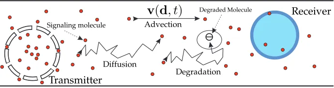
Motivated by natural MC systems, several different me-chanisms have been considered for MC in the literature including free diffusion [6]–[12], gap junctions [13]–[15], molecular motors [16], and bacterial motors [17]; see Fig. 1. In particular, diffusion is referred to as the random movement of small particles suspended in a fluid medium as a result of their collisions with other particles in the fluid. Diffusion is one of the dominant propagation mechanisms in nature including communication inside cells and between cells, e.g., in quorum sensing among bacteria and in the synaptic cleft between neurons. Gap junctions enable another form of communication between cells where the molecules pass through small channels that connect the cytosols of neighboring cells. Calcium signaling is an example of this form of MC that is used by adjacent cells to regulate a large number of cellular processes including fertilization, proliferation, and death of mammalian cells [13], [18]. Molecular motors enable a form of active transportation of large signaling molecules via a special rail-like infrastructure, e.g., actin or microtubule filaments [19]. The motor moves along the rail by using repeated cycles of coordinated binding and unbinding of its legs to the rail. This type of MC is primarily used for intracellular communication among organelles inside a cell [16]. Finally, bacterial motors enable another kind of active transport where the bacteria can pick up large signaling molecules, e.g., deoxyribonucleic acid (DNA), and move in a specific direction, e.g., due to a food concentration gradient, using their tiny propellers (known as flagella) [17].
Diffusion-based MC, sometimes in combination with ad-vection and chemical reaction networks (CRNs), has been the
1We note that, in this paper, we use the terms “molecule” and “particle”
PSfrag replacements
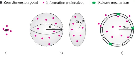
a) b)
c) d)
tx
tx
tx
tx
rx
rx
rx
rx
signaling molecules gap junction channel
rail (e.g. microtubule) molecular motor
food gradient
[image:3.612.101.508.54.260.2]bacterial motor adjacent cells
Fig. 1. Bio-inspired mechanisms for MC between a transmitter (tx) and a receiver (rx); a) Free diffusion, b) gap junctions, c) molecular motors, and d) bacterial motors.
prevalent approach considered in the literature thus far; see [3, Table 4]. The main advantages of diffusion-based MC include that, unlike gap junction-based MC, special infrastructure is not needed, and unlike motor-based MC, external energy for propagation of the signaling molecules is not required. Moreover, the simplicity of diffusion makes it an attractive propagation scheme, especially for ad hoc networks where mobile nanorobots with limited computational resources form a communication network among themselves and/or with living cells in their close proximity. Hence, in this tutorial, we focus on diffusion-based MC, where we also consider environments with advection and CRNs.
A. Scope
The physics of diffusion and characterizing expected diffu-sion in environments of different shapes have been extensively studied in the physics, biology, and chemistry literature, cf. e.g., [20], [21]. Thereby, the primary goal is to understand how natural phenomena work, e.g., to understand the natural and evolutionary MCs that exist within and among living organisms. In contrast, in the emerging field of engineered MC, the aim is to design, build, and control human-made MC systems for a specific purpose2. To this end, the communications research community has expanded the models obtained in other disciplines to account for the behavior of the end-to-end system, for the inclusion of non-diffusive phenomena that play important roles in biophysical systems, and for the statistics of molecular behavior.
Recent surveys, in particular [3], [23], have provided excellent qualitative summaries of diffusive MC and included some of the most common channel models available thus far. A more complete mathematical treatment of diffusion-based
2Different options to build MC systems exist, e.g., to genetically modify
natural cells or to design fully-synthetic MC systems [22]. Therefore, an engineered MC system may also include components that naturally developed via evolution.
modeling of MC can be found in [24]. However, there have been significant advances in channel modeling in the years since the publication of [24], and also since the most recent major survey of models in [3]. In particular, non-diffusive effects that can be coupled with diffusion, such as advective flow and chemical reaction kinetics, have been integrated in many channel models to make them more practical and more accurate.
Due to the rapid growth in channel models, it has become difficult for an interested researcher to enter the MC field and become familiar with the state-of-the-art in diffusion-based channel modeling. It has also become more challenging for practitioners in this field to stay up to date. The aim of this tutorial review is to satisfy both audiences. We present a detailed and rigorous mathematical development of diffusive MC channel models. We seek to provide a useful comprehensive reference on channel models that is both approachable for an audience that is new to the field and also convenient for active practitioners to assess and select a model. To do so, we begin with a review of the underlying fundamental laws that govern diffusive MC channels and show how they are used in the literature to derive the channel impulse responses (CIRs) of different MC systems. In addition, we present different deterministic and statistical models developed for the observation signal at the receiver. We also discuss the complementary roles of simulations and physical experiments to both support analytical modeling and provide data-driven models when simple analytical models that capture the underlying complex dynamics of the system cannot be readily obtained.
B. Contributions
3
components of MC systems. Specifically, we start with Fick’s laws of diffusion and build towards the general advection-reaction-diffusion equation. We discuss the common assumptions and special cases that enable the general equation to be solved for the CIR in closed form. 2) We review the major end-to-end channel models in the diffusive MC literature including the effects of release mechanisms, the physical channel, and reception mecha-nisms. In particular, we include the relevant classical models from the physical sciences literature, as well as a comprehensive presentation of the models that have been developed and the equations that have been derived within the communications engineering community over the last few years.
3) We present a unified definition for the observed signal at a receiver. The unified definition encompasses both timing and counting receivers and helps to better understand the basic assumptions that have been made to arrive at the well-known signal models used in the MC literature and how they relate to each other. Then, we focus on counting receivers and derive signal models relevant for different time scales. We further generalize these models to account for interfering noise molecules and inter-symbol interference (ISI). Finally, we study the correlation between the received signals observed at different time scales.
4) We discuss the integral role of simulations and experi-ments, in particular to gain insight from a data-driven model when closed-form solutions for the CIR are not readily available. We also describe how to implement simple stochastic simulations as well as how to derive an example data-driven model based on experimental data.
For clarity of presentation, the focus of the channel models presented in this work is on a single communication link between one transmitter and one receiver. Many of the envisioned applications of diffusive MC systems will depend on many links within a network of devices. While there have been a number of relevant contributions that consider the propagation of signals over multiple links, such as via relaying and cooperative detection (cf. e.g., [25]–[29]), these models can often be decomposed into a superposition of individual links. In these cases, the analytical models developed in this paper (cf. Sections III and IV) still apply to the individual links. However, it is important to note that single-link analysis cannot always be applied to multi-link systems. For example, when other non-transparent entities (such as reactive receivers) are present in the system and molecules can collide or react with them, each of these entities will impact the signal received atanyreceiver. In general, the impact of other reactive entities on the received signal can be considered by modeling them via additional boundary conditions. Then, the analytical channel modeling methodologies presented in this paper can be used, cf. Sections III and IV. Nevertheless, the resulting systems of partial differential equations (PDEs) are typically too complex to solve and hence, data-driven approaches have to be used in practice, cf. Section V. For example, in [30], the CIR was presented in closed form for the special case of having two
absorbing receivers placed on either side of a transmitter, whereas in [31] a data-driven model was proposed for the more general case of having multiple absorbing receivers at arbitrary positions.
C. Organization
The rest of this tutorial review is organized as follows, and also summarized in Table I to show how the content of Sections II-V is connected. We review the fundamental physical principles that govern diffusion-based MC systems in Section II. In particular, we model diffusion, advection, and chemical reactions, which leads to a general advection-reaction-diffusion PDE to describe the spatio-temporal variation in molecule concentrations.
In Section III, we discuss the components of MC systems and their effect on the to-end CIR. Our definition of the end-to-end channel includes the physical and chemical properties of the transmitter and receiver, as well as the fluid medium in which they are located. A table to summarize the reviewed CIRs is also provided.
In Section IV, we present a unified definition for the diffusive signal observed at the receiver. We focus on counting receivers and derive deterministic and statistical signal models that are valid for different time scales.
We discuss simulation- and experiment-driven models in Section V. We describe the different physical scales for simu-lating diffusion-based systems, summarize existing simulation platforms for each scale, and discuss how to implement simple stochastic simulations. Moreover, we review a selection of experimental platforms and propose to employ either physically-motivated parametric models or neural networks, whose parameters are found using experimental data.
We end this tutorial review with a discussion of future work and open challenges in Section VI before presenting our conclusions in Section VII.
II. FUNDAMENTALGOVERNINGPHYSICALPRINCIPLES IN MC SYSTEMS
In this section, we review the fundamental laws that govern the propagation of molecules. In particular, we mathematically model the impact of diffusion, advection, and reaction on the spatio-temporal distribution of molecules. This modeling is essential for the development of channel models. A solid understanding of these phenomena is needed to develop intuition for molecule propagation in diffusive MC systems. Furthermore, in Section III, we will use the mathematical tools introduced in this section for the derivation of the CIR for several different diffusive MC systems.
A. Free Diffusion
4
TABLE I
ORGANIZATION ANDCONTENT OFSECTIONSII-VANDTHEIRCONNECTIONS.
Section II Governing Physical Principles
Diffusion Advection Reaction
Reaction- Advection-Diffusion Eq.
Section III End-to-End Channel Modeling
Transmitter Channel Receiver
Point Volume Diffusive Advective Degradative Passive Active
End-to-End CIR
Section IV Signal Modeling
Signal Type Three Scales Interference
Timing Counting Deterministic Statistical Time-Varying External ISI
Binomial Gaussian Poisson
Correlation
Sample CIR
Section V Data-Driven Modeling
Simulation Experiment
Continuum Mesoscopic Microscopic Molecular Dynamics
Parametric Model
5
a vector specifying the position of the i-th molecule in three-dimensional (3D) Cartesian coordinates at time t. Thereby, the random walk is modeled by [32, Eqs. (1.3) and (1.21)]
di(t+ ∆t) =di(t) +N(0,2D∆tI), (1)
where∆tis the time step size andDin [m2s−1] is the diffusion coefficient of thei-th molecule. Moreover,N(µ,Σ)denotes a multivariate Gaussian random variable (RV) with mean vector
µ and covariance matrix Σ, 0 represents a vector whose elements are all zeros, andIis the identity matrix. The diffusion coefficient determines how fast the molecule moves. The larger the diffusion coefficient, the larger the average displacement of the molecule in a given time interval. The value of the diffusion coefficient depends on the environment as well as the shape and the size of the particle. For spherical particles immersed in a fluid continuum, the diffusion coefficient can be determined based on the Einstein relation [33, Chapter 5.2.1]
D= kBT
6πηR, (2)
wherekB= 1.38×10⁻²³JK−
1 is the Boltzmann constant,T
is the temperature in kelvin,η is the (dynamic) viscosity of the fluid (η= 10−3 kg m−1s−1 for water at 20◦C), andRis the
radius of the particle. Note that larger particles have a smaller diffusion coefficient and are hence less affected by diffusion. Remark 1:From [33, Chapter 5.2.1], the diffusion coefficient can be determined from (2) as long as the surrounding liquid can be modeled as a continuum. By experiment, this is an accurate assumption if the particle size is at least five times the size of the molecules of the liquid. For example, in water, (2) is applicable for particles having a diameter larger than
1.5 nm. For small particles not satisfying this condition, the diffusion coefficient tends to be larger than that predicted by (2). Nevertheless, a general formula encompassing all physical
regimes does not exist.
Remark 2: Besides the ideal free diffusion with constant diffusion coefficient discussed above, there are also other types of diffusion. For instance, in contrast to the typical free diffusion where the mean squared displacement (MSD) is linearly proportional to time, i.e., MSD ∝ D∆t, in anomalous diffusion, the MSD follows a nonlinear relation, i.e., MSD∝D∆tγ whereγ6= 1. Sub-diffusion occurs when γ <1and can be used to model diffusion inside biological cells where the presence of the organelles does not allow ideal free diffusion to take place [34]. Super-diffusion occurs whenγ >1
and can be used to model active cellular transport processes [35]. Moreover, in (1), we assumed the diffusion coefficient to beconstant. However, the diffusion coefficient may depend on the local concentration of the molecules [33]. For the constant diffusion coefficient assumption to hold, the temperature and viscosity of the environment are assumed to be uniform and constant and all solute molecules (dissolved molecules) are assumed to be locally dilute everywhere, i.e., the number of solute molecules is sufficiently small everywhere. These assumptions allow us to ignore potential collisions between solute molecules such that the diffusion coefficient does not vary with the local concentration [8], [33]. We refer the readers to [36] for the study of diffusion with non-constant diffusion
coefficients. Another example of a complex diffusion process is the diffusion of protons in water. Here, the movement of the protons is a combination of ideal free diffusion and the so-called structural diffusion where protons hop from one water molecule to the next. Nevertheless, it has been shown in [37] that proton transport can be well approximated by free diffusion
with an effective diffusion coefficient.
We letc(d, t)denote the concentration of the solute mole-cules, i.e., the average number of solute molecules per unit volume, at coordinatedand timet. The random movement of molecules due to diffusion, described by (1), leads to variation of c(d, t)across time and space that obeys Fick’s second law of diffusion3
∂c(d, t) ∂t =D∇
2c(d, t), (3)
where∇2 is the Laplace operator, e.g.,∇2= ∂2
∂x2+
∂2
∂y2+
∂2
∂z2
in Cartesian coordinates. The PDE in (3) can be solved for simple initial conditions (ICs) and simple boundary conditions (BCs). In the following, we consider a simple example, namely diffusion in an unbounded 3D environment with an impulsive point release, which has been the most widely studied case in the MC literature due to its simplicity [3], [38]–[46]. In the remainder of this paper, we denote the solutions of the considered PDEs byc∗(d, t).
Example 1 (Diffusion in an Unbounded 3D Environment with Impulsive Point Release):Consider a 3D diffusion process with instantaneous release of N solute molecules fromd0 at time t0. To obtainc∗(d, t), we have to solve (3) with the following
initial and boundary conditions
IC1: c(d0, t→t0) =N δ(d−d0) (4)
BC1: c(kdk → ∞, t) = 0, (5)
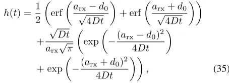
where δ(d) = δ(x)δ(y)δ(z), and δ(·) is the Dirac delta function. Solving (3) withIC1 and BC1 yields [32, Eq. (2.8)]
c∗(d, t) = N
(4πD(t−t0))3/2exp
−kd−d0k
2
4D(t−t0)
. (6)
In Fig. 2, the molecule concentration c∗(d, t)
molecules/m3
in (6) is plotted versus time [µs] at distance d = [d,0,0] with d ∈ {300,400,500} nm for an initial release ofN = 104 molecules with D= 4.5
×10−10
m2/s from the origind0= [0,0,0]at timet0= 0. From Fig. 2,
we observe that first c∗(d, t)increases with time, which is due
to the non-zero propagation time that the molecules need to reachd, before it decreases since the molecules diffuse away. Moreover, as distance increases, the peak of the concentration decreases since the molecules are spread over a larger volume. Furthermore, the time when the concentration peak occurs, denoted by tp, increases with distance.
The assumption of an unbounded environment is accurate when the actual boundaries of the system are far away from the region of interest (i.e., from transmitter and receiver), such that the impact of the boundaries on the diffusing molecules
3Fick’s first law of diffusion relates the diffusive flux, denoted byJ(d, t),
d= 500nm
d= 400nm
d= 300nm
c
∗(d
,t
)
×
10
−
21
[m
o
le
cu
le
s/
m
3]
Time [µs]
0 100 200 300 400 500
[image:7.612.59.291.72.257.2]0 5 10 15 20 25 30
Fig. 2. Molecule concentrationc∗(d, t)
molecules/m3
versus time [µs] at distanced = [d,0,0]withd∈ {300,400,500} nm for initial release of N = 104 molecules with D = 4.5×10⁻¹⁰ m2/s from the origin d0= [0,0,0]at timet0= 0.
can be neglected. In the following, we present an example where the effect of the boundaries cannot be neglected.
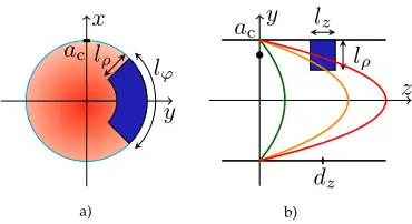
Example 2 (Diffusion in an Unbounded Straight Duct with Impulsive Release from Cross-Section):We assume a straight duct4 channel with circular cross-section and for convenience, we employ cylindrical coordinates, i.e., d = [ρ, ϕ, z] with
0≤ρ≤ac, 0≤ϕ≤2π,−∞< z <+∞, whereac denotes
the radius of the circular cross-section of the duct. We assume that, at the time of release, t0, the molecules are uniformly
distributed across the cross-section atz=z0. Therefore, we
have the following initial and boundary conditions
IC2:c(d0= [ρ, ϕ, z], t→t0) = N πa2
c
δ(z−z0) (7)
BC2: ∂c(d, t) ∂ρ
ρ=a
c
= 0 (8)
BC3:c(d= [ρ, ϕ, z→ ±∞], t) = 0, (9)
whereBC2enforces the reflection of the molecules at the wall, i.e., a fully reflective wall is assumed. Solving (3) with IC2,
BC2, andBC3 yields [47]
c∗(d, t)
= N
πa2 c
p
4πD(t−t0))exp
− (z−z0)
2
4D(t−t0)
, ρ < ac.(10)
As can be seen from (10), c∗(d, t) does not depend on
variables ρandϕdue to the symmetry of the initial condition and the environment with respect to ρandϕ. This model can be used to characterize the propagation of molecules in blood vessels as is necessary for drug delivery applications of MC in the cardiovascular system [48]–[52].
4A duct is a pipe, tube, or channel which carries a liquid or gas.
B. Advection
Besides diffusion, advection is another fundamental mecha-nism for solute particle transport in a fluid environment. In the following, we first specify how mass transport by advection affects a single solute particle. Subsequently, we distinguish between two types of advection, namely drift and fluid flow, and give the particle velocity vector for some example cases. Moreover, we present the advection equation which describes the change in molecule concentration due to advection. Finally, we introduce the advection-diffusion equation, which captures the joint impact of diffusion and advection, and characterize the relative importance of diffusion and advection.
In general, transport by advection can be described by a velocity vectorv(d, t)which generally may depend on position d and time t. When considering the movement of the i-th particle at position di due to advection, its position at time t+ ∆t can be modeled by
di(t+ ∆t) =di(t) +v(di(t), t)∆t, (11)
where∆tshould be small enough such that the velocity vector is constant betweendi(t)and di(t+ ∆t). Next, we discuss what may cause the velocity vectorv(d, t)and what form it may take.
1) Velocity Vector Field: Transport by advection can be mediated by different physical mechanisms which we categorize as force-induced drift andbulk flow[53], [54].
Force-Induced Drift:Advection can be caused by external
forces acting on the particles but not on the fluid containing the particles. An external force can be modeled by force vector F(d, t) which describes the force on a particle at position d at time t. These external forces can be electrical, e.g., if the particles are ions, or magnetic, e.g., if the particles are magnetic nanoparticles, or gravitational, e.g., if the particles have sufficient mass, or a combination of forces [54], [55]. When the force is not too large, the velocity vector can be determined from the corresponding force by Stokes’ law via [56, Eq. (2.65)]
v(d, t) =F(d, t)
ζ , (12)
whereζ is a proportionality constant referred to as the friction coefficient. The friction coefficient can be related to the diffusion coefficient via ζD = kBT. In other words, using (2), we obtainζ= 6πηR. ForceF(d, t)may vary with time (e.g., for ions if the electric field changes over time) and space (e.g., for magnetic nanoparticles, the magnetic force generally decreases rapidly with increasing distance from the magnet) [54], [55].
Bulk Flow: If the particle movement is induced by the
7
The flow may also depend on time, e.g., in a blood vessel the flow is generated by the periodic contractions of the heart.
Remark 3: Although both flow and external force cause the particles to drift, which can be modeled by (11), they may require quite different considerations. For instance, any object in the environment influences the velocity vector caused by bulk flow since the flow may not be able to penetrate the object and has to go around the object. On the other hand, the drift velocity vector caused by an external force is not necessarily
influenced by objects in the environment.
Flow can be also categorized into two classes, namely turbulent andlaminar flow. In particular, when the variations of the flow velocity, over space and/or time, are stochastic, e.g., due to rough surfaces and high flow velocities [58], we refer to the flow as turbulent. If the flow is not turbulent, it is referred to as laminar. For flow in a bounded environment of effective length deff and with an effective velocity ofveff,
the Reynolds number can be used as a criterion for predicting laminar or turbulent flow and is given by [58, Eq. (1.24)]
Re = deff ·veff
ν , (13)
where ν is the kinematic viscosity [m2/s] of the fluid5. For example, for flow in a straight pipe with circular cross-section of radius ac, the flow can be assumed to be laminar and
turbulent for Re2100andRe2100, respectively, where
deff =ac [58]. For microfluidic settings, typically Re10
and hence laminar flow can be assumed [56]. For most blood vessels,Re<500 holds and hence the blood flow is typically laminar [59], [60]. Only in large arteries such as the aorta (the largest artery in the human body), the Reynolds number can be in the range [3400,4500] and thereby blood flow exhibits turbulent behavior [60].
Generally, for a given environment, the flow velocity vector v(d, t)as a function of space and time can be determined by solving the so-called Navier-Stokes equation with appropriate boundary conditions, see e.g. [56, Eq. (5.22)]. Let us review two special cases of v(d, t), which have been widely studied in the MC literature [3], [44], [53], [61], [62] and are also considered in Section III.
Example 3 (Uniform and/or Constant Advection): For
uniform advection, the velocity vector is constant across space but can be time-dependent, i.e., v(d, t) = v(t) [62]. For advection by flow in an unbounded environment, uniform flow solves the Navier-Stokes equation and hence can be physically plausible. Moreover, for advection by drift, uniform drift is applicable when the corresponding force vector does not depend on space, see (12). As a special case, the velocity vector may be constant across both space and time, i.e., v(d, t) =v. Due to its simplicity, advection with constant velocity is the most widely-studied advection model in the MC literature [3], [44],
[53].
Example 4 (Steady Flow in an Infinite Straight Duct with Circular Cross-Section): For this example, we concentrate on advection by fluid flow because force-induced drift is completely specified by (12). In particular, in this case, the
5Kinematic viscosityν is related to (dynamic) viscosityη according to
ν=η/ρdwhereρd[kg m−3] is the fluid density.
flow velocity vector in cylindrical coordinates[ρ, ϕ, z] can be obtained as [58, Eq. (4.134)]
v(ρ) =
0,0, v0
1−ρ 2
a2 c
, 0≤ρ≤ac, (14)
where v0 is the center velocity. The flow described in (14)
is laminar and can be interpreted as follows. For a given ρ, the flow velocity in (14) is constant but increases from the boundary where v(ac) = [0,0,0] towards the center where
v(0) = [0,0, v0], i.e., for each ρ, we can think of a circular layer within the duct that slides along its neighboring layers with a constant velocity. The velocity vector in (14) is known as the Poiseuille flow profile and is a common model for the
flow in blood capillaries [61].
While for other environments and boundary conditions the velocity vector can still in principle be obtained from the Navier-Stokes equation, it is often not possible to do so analytically. In these cases, the Navier-Stokes equation can be solved by numerical algorithms that are well-established in computational fluid dynamics [58].
2) Advection Equation: Givenv(d, t), the change in con-centration with respect to time due to advective transport is modeled by the following PDE, which is referred to as the advection equation or continuity equation [56, Eq. (4.14)]
∂c(d, t)
∂t =−∇ ·(v(d, t)c(d, t)), (15)
where∇= [∂x∂ ,∂y∂ ,∂z∂ ]denotes the gradient operator andx·y denotes the inner product of two vectorsxandy. In general, (15) cannot be readily solved for a given velocity vector and numerical methods have to be employed [63]. Nevertheless, for the velocity vectors in Examples 3 and 4, (15) can be solved as shown in the following.
Example 5:Assuming initial conditionc(d,0)att= 0, the advection equation (15) has the following solution for t >0
c∗(d, t)
=
c
d−
Z t
0
v(τ) dτ,0
, Uniform Flow
c(d−vt,0), Constant Uniform Flow
c(d−v(ρ)t,0), Poiseuille Flow.
(16)
We note that while the solutions in (16) appear similar, they are actually fundamentally different. In particular, for constant uniform flow and uniform flow (space-independent flow profiles), the initial concentration is simply translated to a different position without changing its shape. However, for Poiseuille flow (space-dependent flow profile), the concentra-tion generally spreads in space over time depending on the initial concentration.
3) Advection-Diffusion Equation: In many application scena-rios, such as drug delivery via the capillary networks [48]–[52], advection and diffusion are both present in the MC environment. Thereby, the combined effect of both advection and diffusion is characterized by the following PDE known as the advection-diffusion equation
∂c(d, t) ∂t =D∇
2c(d, t)
v= 5×10⁻³m/s v= 2×10⁻³m/s v= 0
c
∗(d
,t
)
×
10
−
21
[m
o
le
cu
le
s/
m
3]
Time [µs]
0 100 200 300 400 500
[image:9.612.59.291.71.256.2]0 10 20 30 40 50 60
Fig. 3. Molecule concentrationc∗(d, t)[molecules/m3] versus time [µs] at
d= [400,0,0]nm for initial release ofN= 104molecules withD= 4.5×
10−10m2/s fromd
0= [0,0,0]att0= 0, and flow velocityv= [v,0,0]
withv∈ {0,2,5} ×10−3m/s.
Similar to diffusion equation (3), (17) cannot be solved analytically for general velocity vectors v(d, t)and general boundary and initial conditions. In the following, we first provide the solution of (17) for constant uniform flow in an unbounded environment. Subsequently, we quantify the relative impact of diffusion over advection by introducing the notions of P´eclet number and dispersion factor.
Example 6: Consider an unbounded 3D environment with instantaneous release of N solute molecules at d0 at time t0. Solving (17) with initial condition IC1 in (4), boundary
condition BC1 in (5), and constant uniform velocity vectorv yields [44, Eq. (18)]
c∗(d, t) = N (4πD(t−t0))3/2
×exp
−kd−(t−t0)v−d0k
2
4D(t−t0)
, t > t0.(18)
In Fig. 3, we show molecule concentration c∗(d, t)
[molecules/m3] in (18) versus time [µs] atd= [400,0,0]nm for initial release ofN = 104molecules withD= 4.5×10⁻¹⁰
m2/s from d0= [0,0,0] att0= 0, and flow velocity vector
v= [v,0,0]with v∈ {0,2,5} ×10−3 m/s. From Fig. 3, we
observe that as the flow velocity increases, the concentration peak increases andtpdecreases. This is mainly due to the fact
that the flow is in the same direction as the point where the concentration is measured, i.e., parallel flow is considered. Parallel flow can considerably enhance the coverage of a diffusion-based MC system, e.g., in blood vessels. Moreover, by increasing v, the tail of c∗(d, t) over time is decreased,
which is useful for ISI reduction in MC systems [44], [64]. Relative Importance of Advection over Diffusion for
Mo-lecule Transport:Advection and diffusion can both displace
and transport molecules, albeit in different ways. An important
question is under what conditions is one more effective than the other. The P´eclet number, denoted byPe, can be used to answer this question. Let us assume a velocity vector with strengthv and transport over a distancedc which is referred to as the characteristic length. The P´eclet number quantifies the ratio of time required for particles to be transported by diffusion over distancedc(which is proportional tod2c/D) with the time required for particles to be transported by advection over distancedc (given by dc/v). This ratio is given by [56, Eq. (4.44)]
Pe =
d2
c
D dc
v
= v·dc
D . (19)
Note that Pe is a dimensionless number. If Pe 1 holds, diffusion dominates advection and the spreading of molecules is almost isotropic despite a weak biased transport in the direction of the flow. In this case, the solution of the diffusion equation (3) provides an accurate estimate of the molecule concentration. On the other hand, if Pe 1 holds, advection dominates diffusion and is the main cause for molecule transport. In this case, the advection equation (15) can be solved to obtain an accurate estimate of the molecule concentration. Finally, for
Pe≈1, molecule transport is sensitive to both diffusion and advection and the advection-diffusion equation in (17) should be solved.
Relative Importance of Advection over Diffusion for
Dispersion: Let us consider a straight duct with a circular
cross-section, see Examples 2 and 4, where advection is the main transport mechanism along the duct. In other words,
Pez, veffDdz 1holds where Pez denotes the P´eclet number for transport along the z-axis, veff = v0/2 is the effective
flow velocity in the duct (see (14)), and dz is the desired transport length along thez-axis. In this case, we are interested in studying the dispersion (spatial spreading) of individual particles across the cross-section over the time when transport along the z-axis occurs. In particular, one may distinguish between the following two extreme regimes, namely the non-dispersive and non-dispersive regimes:
i) Non-dispersive regime:Here, particles do not considerably diffuse across the cross-section while being transported by advection. Therefore, each particle is simply transported along the z-axis by advection with a velocity strength that depends on the radial position of the particle, ρ, according to (14). We note that although the dispersion of individual particles is negligible in this regime, the shape of the concentration profile varies over time since the flow has a different effect at different radial positions, i.e., particles closer to the center of the duct travel faster.
ii) Dispersive regime:In the dispersive regime, particles fully diffuse across the cross-section while also being transported along the z-axis by advection. In addition to the dispersion across the cross-section, there is also dispersion along thez -axis, due to the combined impact of diffusion and advection with space-dependent flow profile (14).
9
(usually a fraction of ac). Moreover, we defined¯z ,dz/dc as the corresponding dimensionless normalized distance with respect to characteristic distance dc. Then, we can compare the characteristic time required for particles to be transported by advection over distancedz (given bydz/veff) with the time
required for diffusion over distancedc (which is proportional to d2
c/D). To compare these two time scales, we can define a dispersion factor αd as
αd= dz
veff
d2
c
D
= Ddz veffd2c
= d¯ 2
z
Pez
. (20)
Here, αd 1 signifies that there is not enough time for particles to diffuse across the cross-section while being transported by advection over distance dz, i.e., we are in the non-dispersive regime. On the other hand, forαd1, diffusion causes considerable dispersion across the cross-section, which in turn causes significant dispersion along the z-axis due to space-dependent flow velocity (14), i.e., we are in the dispersive regime. In other words, in terms of the P´eclet numberPez, we have non-dispersive and dispersive regimes if Pezd¯2z and
Pezd¯2z hold, respectively.
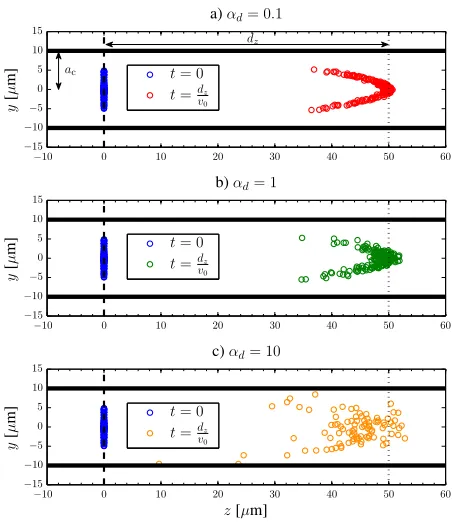
Fig. 4 illustrates different dispersion regimes for a 3D straight duct. For clarity of presentation, we only show those particles for which the x-component of their position lies in interval
[−0.1ac,0.1ac]. As can be seen from Fig. 4, for αd = 0.1, the positions of the particles simply follow the velocity profile in (14) whereas for αd = 10, the particles are significantly dispersed in the environment.
C. Chemical Reactions
Another important phenomenon affecting the propagation of signaling molecules in diffusive MC systems is chemical reactions. On the one hand, chemical reactions may occur naturally in MC environments and their impact must be taken into account for communication design. On the other hand, chemical reactions have been exploited in the MC literature to achieve certain objectives, such as ISI reduction [43], [44], [65], [66] and ligand-based reception modeling [67], [68]. Therefore, in the following, we first review general chemical reactions, the corresponding reaction equations, and examples of reactions widely considered in the MC literature. Subsequently, we study the joint impact of all three phenomena discussed in this section, namely diffusion, advection, and reaction, on the propagation of the molecules and solve the corresponding advection-reaction-diffusion equation for a simple example.
1) Reaction Equation: Consider a general reaction of the form [69, Eq. (13)]
X
I∈I nII
κ
→ X
J∈J
nJJ, (21)
where I∈ I are reactant molecules,I is the set of reactant molecules, J ∈ J are product molecules, J is the set of product molecules, nI and nJ are non-negative integers, and κis the reaction rate constant. Let cI(d, t)and cJ(d, t) denote the concentration of type-I and type-J molecules at coordinatedand timet, respectively. Reactions locally change
PSfrag replacements
dz
ac
t=dz
v0 t= 0
c)αd= 10
y
[
µ
m
]
z[µm] t=dz
v0 t= 0
b)αd= 1
y
[
µ
m
]
t=dz
v0 t= 0
a)αd= 0.1
y
[
µ
m
]
−10 0 10 20 30 40 50 60
−10 0 10 20 30 40 50 60
−10 0 10 20 30 40 50 60
[image:10.612.324.550.70.331.2]−15 −10 −5 0 5 10 15 −15 −10 −5 0 5 10 15 −15 −10 −5 0 5 10 15
Fig. 4. Illustration of different dispersion regimes in a 3D straight duct with reflective walls,D= 10−11m2/s,a
c= 10µm,dc = 0.1ac,dz = 50µm,
the flow velocity profile in (14), andv0= 10−2,10−3,10−4m/s which leads
toαd= 0.1,1,10, respectively. For clarity of presentation, we only show
particles whosex-component of the position lies in interval[−0.1ac,0.1ac].
The particles are initially placed atz = 0and uniformly distributed in a disk with radius5µm centered at(x, y) = (0,0). The solid horizontal lines represent the duct walls, the dashed vertical lines denote the initial positions of the particles on thez-axis, and the dotted vertical lines denote the distance of interest on thez-axis, i.e.,dz.
the concentration of particles over time which is described by the following PDEs, known as reaction equations
∂cI(d, t)
∂t =−nIf(κ, cI,∀I∈ I), ∀I∈ I (22a) ∂cJ(d, t)
∂t =nJf(κ, cI,∀I∈ I), ∀J ∈ J, (22b)
where f(κ, cI,∀I ∈ I) denotes the reaction rate function, which depends on the reaction rate constant and the concen-trations of the reactant molecules. The reaction rate function has the following general form, known as the rate law [70, Eq. (9.2)]
f(κ, cI,∀I∈ I) =κ Y
I∈I cεI
I (d, t), (23)
where εI is the order of the reaction with respect to type-I reactant molecules and typically takes an integer value (but in principle may also assume real values). The overall reaction order is defined asP
I∈IεI [47], [70]. Note that the units of reaction rate functionf(κ, cA, cB)and reaction rate constant κare molecules·m3 and
1
s molecule
m3
1−PI∈IεI
, respectively.
is a natural characteristic of some types of molecules and its effect has to be accounted for in communication design, see Section III-D and [44], [71]. Bimolecular reactions can be used to analayze ligand-receptor binding [67], [68] and reactive signaling [66], [74]. Enzymatic reactions have been studied in the MC literature for the purpose of ISI reduction [65], [73]. Example 7 (Unimolecular Degradation): This reaction is used to describe the degradation of a desired type of molecule, e.g., type A, into a new type of molecule, denoted by φ, which is of no interest for the considered communications. In fact, unimolecular degradation is often used as a first-order approximation of more complex reactions such as bimolecular and enzymatic reactions, see Examples 8 and 9. Unimolecular degradation is modeled by [70, Ch. 9]
A→κ φ, (24)
where κ [1s moleculem3
1−εA
] is the reaction rate constant,
f(κ, cA) =κcAεA(d, t)is the reaction rate function, andεA is the reaction order. In the MC literature, first-order reactions are used to model degradation, i.e., εA= 1 [44], [71]. However, depending on the speed of reaction, higher and lower order reactions may be relevant, e.g., zero-order (εA= 0) or second-order (Type-I) (εA = 2) reactions [70, Ch. 9]. Assuming an initial conditioncA(d, t0)att0, (22) has the following solution
for t > t0
c∗A(d, t) =
[cA(d, t0)−κ(t−t0)]+, if εA= 0 cA(d, t0) exp(−κ(t−t0)), if εA= 1
1/(κ(t−t0) + 1/cA(d, t0)), if εA= 2, (25)
where [x]+ = max
{0, x}. Note that the speed of molecule concentration decay is hyperbolic for second-order degrada-tions, which is faster than the exponential decay for first-order degradations, which in turn is faster than the linear decay for zero-order degradations. Nevertheless, for sufficiently large t,c∗A(d, t)for second-order degradations is larger than that for first-order degradations, whereas c∗A(d, t) = 0, t≥ t0+cA(d,tκ 0), holds for zero-order degradations.
Example 8 (Bimolecular Reactions): Some reactions may involve the interaction of two reactant chemical species, e.g.,A
andB, to produce product molecule(s), e.g.,C. For instance, in [67], the activation of ligand receptors via signaling molecules was modeled by a second-order bimolecular reaction. Moreover, in [66] and [74], acids and bases were used as reactive signaling molecules to reduce ISI. Acids and bases cancel each other out to produce salt and water. This process is modeled by a order bimolecular reaction. In particular, the second-order (Type-II) bimolecular reaction is given by [75]
A+B κf
κb
C, (26)
whereκf is the forward reaction rate constant m3
s·molecule
,κb 1
s
is the backward reaction rate constant, andf(κ, cA, cB) = κfcA(d, t)cB(d, t) is the reaction rate function. The PDEs corresponding to (26) are nonlinear and challenging to solve. However, after introducing some approximations, in Section III, we use (26) to derive the CIRs of MC systems affected by bimolecular reactions. Moreover, let us assumeκb→0and that
the concentration of type-Bmolecules is sufficiently large such that the reaction in (26) does not considerably changecB(d, t) over time, i.e.,cB(d, t)≈cB(d, t= 0),cB(d). In this case, the bimolecular reaction in (26) can be approximated by the first-order unimolecular reaction in (24) with κ= κfcB(d)
[67].
Example 9 (Enzymatic Reactions):For typical scenarios, the speed of natural degradation might be too slow compared to the desired time scale of communication. In this case, enzymes can be used to accelerate the reaction process. Enzymes, denoted byE, are specific proteins that bind to the desired molecule
A(also referred to as the substrate), and lower the activation energy needed for a reaction to occur. Enzymatic degradations are modeled by the following reactions [65, Eq. (1)]
A+Eκf
κb
AE κd
→E+φ, (27)
where AE is an intermediate chemical species and φ is the product molecule. Moreover,κf m
3
s·molecule
,κb1s, andκd1s denote the reaction rate constants of the forward, backward6, and degradation reactions, respectively. As can be seen from (27), the enzyme molecules are notconsumed in the reaction process. The following set of PDEs, known as Michaelis-Menten kinetics, describe the evolution of the concentrations of the participating molecules
∂cA(d, t)
∂t =−κfcA(d, t)cE(d, t) +κbcAE(d, t) (28a) ∂cE(d, t)
∂t =−κfcA(d, t)cE(d, t) + (κb+κd)cAE(d, t)(28b) ∂cAE(d, t)
∂t =κfcA(d, t)cE(d, t)−(κb+κd)cAE(d, t).(28c)
Solving the above system ofcoupledandnonlinear PDEs is challenging. Let us consider very fast degradation reactions, i.e., κd → ∞, slow backward reactions, i.e., κb → 0, and that the concentration of enzyme molecules is much larger than the concentration of type-A molecules. In this case, the formation of intermediateAEmolecules does not last long and hence, we obtaincE(d, t)≈cE(d, t= 0),cE(d). In [65], it was shown that under the aforementioned assumptions, the enzymatic reaction in (27) can be approximated by the first-order unimolecular reaction in (24) with reaction rate constant
κ= κfκd
κb+κdcE(d)≈κfcE(d).
2) Advection-Reaction-Diffusion Equation: Next, we con-sider the joint effects of diffusion, drift, and reactions. For simplicity, we focus on a single molecule type and drop the corresponding subscript. In this case, the general advection-reaction-diffusion equation is given by the following PDE [32], [76]
∂c(d, t) ∂t =D∇
2c(d, t)
−∇ ·(v(d, t)c(d, t)) +qf(κ, c(d, t)), (29)
where q = 1 and q = −1 hold if the considered molecule is the product and the reactant of the reaction, respectively. Solving (29) for general initial and boundary conditions is
6The forward and backward reaction rate constants are also referred to as
11 PSfrag replacements
κ= 2×1041/s κ= 1041/s κ= 0
c
∗(d
,t
)
×
10
−
21
[m
o
le
cu
le
s/
m
3]
Time [µs]
0 100 200 300 400 500
0 2 4 6 8 10 12 14 16 18 20
Fig. 5. Molecule concentration c∗(d, t)[molecules/m3] versus time [µs]
atd = [400,0,0]nm for an initial release of N = 104 molecules from
d0 = [0,0,0] and at t0 = 0, D = 4.5×10⁻¹⁰ m2/s, flow velocity
v= [10−3,0,0]m/s, andκ∈ {0,1,2} ×1041/s.
again difficult for most practical MC environments. Hence, in the following, we make some simplifying assumptions that enable us to solve (29) in closed form for one example scenario [65].
Example 10: Let us assume the impulsive release of N
molecules at time t0 by a point source located atd0 into an
unbounded 3D environment, i.e., initial condition IC1 in (4) and boundary conditionBC1in (5) hold. Moreover, we assume uniform flow v(d, t) = v and the first-order degradation reaction in (24), i.e., q = −1 and f(κ, c(d, t)) = κc(d, t). Based on these assumptions, (29) has the following closed-form solution [77], [78]
c∗(d, t) = N (4πD(t−t0))3/2
×exp
−κ(t−t0)−kd−(t−t0)v−d0k 2
4D(t−t0)
, t > t0.(30)
In Fig. 5, the molecule concentrationc∗(d, t)[molecules/m3]
is shown versus time [µs] at d= [400,0,0]nm for an initial release of N= 104 molecules fromd
0= [0,0,0]and att0= 0,D= 4.5×10⁻¹⁰ m2/s, flow velocityv= [10−3,0,0]m/s,
and κ ∈ {0,1,2} ×104 1/s. This figure shows that as the
degradation rate constant increases, the concentration peak decreases, which is not desirable for an MC system, in general. However, the tail of the concentration for larget fades away much faster for larger degradation rates, which was exploited for ISI reduction in [65].
III. COMPONENTMODELING
In this section, we review the existing component models for the transmitter, receiver, and physical channel of diffusive MC systems. To this end, in Section III-A, we first define the end-to-end CIR of single-link diffusive MC systems, and
discuss the relevant mechanisms of each component and their impact on the end-to-end CIR. We use the CIR to characterize the components of MC systems, since the impulse response fully characterizes the behavior of linear systems, and linearity is commonly assumed in the MC literature7. Subsequently, in Sections III-B, III-C, and III-D, we review the existing models that have been developed by taking into account the impact of the receiver, transmitter, and physical channel on the end-to-end CIR, respectively. Finally, in Section III-E, we provide a summary table of all reviewed end-to-end CIR models.
A. Channel Impulse Response
In this subsection, we first briefly discuss the relevant me-chanisms that characterize the functionalities of the transmitter and receiver, and the phenomena and impairments that occur in the physical channel of diffusive MC systems. Then, we provide a formal definition of what we refer to as the end-to-end channel of diffusive MC systems and we show how the CIR corresponding to the end-to-end channel can be obtained using the tools introduced in Section II.
Similar to traditional communication systems, the end-to-end chain of diffusive MC systems consists of three components, namely the transmitter, the physical channel, and the receiver; see Fig. 6. Each of these components has unique features and responsibilities, which are outlined below; see also Fig. 7.
• Transmitter: The transmitter is responsible for the
en-coding and modulation of information bits. In MC, the information is typically encoded in the number, type, or time of release of signaling molecules. Furthermore, the transmitter has to generate the signaling molecules (e.g. by CRNs inside the transmitter), store the signaling molecules (e.g. in vesicles), and control their release into the physical channel.
• Physical Channel: The physical channel is the
envi-ronment in which the signaling molecules move and propagate once they leave the transmitter. In diffusive MC systems, the movement of signaling molecules, at its most basic level, is described by the diffusion process. However, during the course of diffusion, the random walk of signaling molecules may be affected by several other factors and noise sources such as advection, CRNs degrading the signaling molecules, environment geometry, and obstacles inside the physical channel, see Section II.
• Receiver:Signaling particles that reach the vicinity of the
receiver can be observed and processed by the receiver to extract the information that is necessary for performing detection and decoding. The reception mechanism of the receiver may include the following functionalities, depending on its structure: i)external sensory units for detecting the presence of signaling molecules, membrane receptors of cells in nature, or sensing component(s) of macro-scale receivers such as the alcohol sensor in
7Linear models of MC systems provide first-order approximations of the
[image:12.612.59.292.73.256.2]Fig. 6. Schematic presentation of the end-to-end chain of communication in typical diffusive MC systems.
Fig. 7. Example of a physical system model including a transmitter, physical channel, and receiver.
[64] and the magnetic coils of the susceptometer in [79]; ii) internal relaying and interface components to convey and convert the measurements of the sensory unit into quantitites suitable for detection and decoding of the information bits. For instance, in nature, this task is performed by the CRNs insidecells, which are referred to as downstream signaling pathways [18]. Downstream signaling pathways may be driven by activated receptors or directly by signaling molecules that passively enter the cells.
In the following, we formally define the end-to-end channel to study the reviewed CIR models in a unified manner.
Definition 1 (End-to-end Channel): We define the end-to-end channel as the effective channel that not only includes the physical channel but also the impact of the physical and chemical properties of the transmitter and receiver, including the effects of signaling molecule generation, release mechanisms, sensory units, and internal receiver components. Note that our definition of the end-to-end channel does not include the coding, modulation, detection, and decoding operations that the transmitter and receiver may perform; see also Fig. 6. This definition of the end-to-end channel is analogous to that in traditional wireless communication systems, where the antennas, power amplifiers, and filters of the transmitter and receiver are also included in the model for the wireless end-to-end channel. The input to the end-to-end channel is the signal representing the modulated information symbol, which we also refer to as the stimulation signal. The stimulation signal can be an electrical (voltage or current), magnetic, mechanical, optical, chemical, or temperature signal. The output of the end-to-end channel is referred to as the observed signal and should be in a form that is suitable for the subsequent detection and decoding operations. Depending on the structure of the receiver, the observed signal can be either a number ofoutput molecules or any secondary signal derived
from the output molecules. In particular, output molecules may represent:i) signaling molecules that can passively enter the receiver;ii)absorbed molecules that hit the receiver surface; oriii)activated receptors. Furthermore, the secondary signal derived from output molecules may be an electrical signal, e.g., the output voltage or output current of the alcohol sensor in [64]. In the following, for the definition of the CIR of the end-to-end channel, we emphasize that we consider the number of output molecules as the observed signal, as it is commonly assumed in the MC literature, although our definition can be easily extended to other forms of the observed signal.
Definition 2 (Channel Impulse Response): We define the CIR of the end-to-end channel, denoted by h(t), as the probability ofobservationof one output molecule at timet at the receiver when the transmitter is stimulated in an impulsive
manner at timet0= 0.
We note that defining the CIR as a probability has several advantages. In particular, it facilitates the definition of the received signal in Section IV. There, we propose a general received signal model that takes into account both thearrival time and the numbers of observed output molecules. As is shown in Section IV, both of these quantities can be readily obtained from the probability of observation of one output molecule.
[image:13.612.133.478.193.284.2]13
In this section, we assume that the parameters of the considered MC system are constant, i.e., the end-to-end CIR
h(t)is time-invariant. In the following, we refer to the signaling molecules as A molecules. The following phenomena may affect the propagation of the A molecules, and as a result,
h(t):
1) Particle generation: Generation of the A molecules is
performed, e.g., by the CRNs inside the transmitter.
2) Release mechanism: The release mechanism can be
chemical, electrical, or mechanical and controls the release of the Amolecules into the physical channel.
3) Diffusion:Diffusion refers to the propagation of
molecu-les by Brownian motion.
4) Degradation and production: CRNs may degrade or
produce Amolecules in the physical channel.
5) Advection: Advection may affect the transportation of
the Amolecules in the physical channel.
6) Geometry: Potentially, the geometry of the individual
components of the end-to-end channel can influence the propagation of signaling molecules.
7) Receptor kinetics:Receptor kinetics affect the interaction
of the Amolecules with the receptors of the sensory unit at the receiver.
8) Signaling pathways:The signaling pathways transducing
the observedA molecules into a secondary signal affect the received signal.
In order to obtain h(t) for a specific MC system, one has to solve the advection-reaction-diffusion equation (29) or a simplified version thereof, depending on the MC system under consideration, with the appropriate initial and boundary conditions. The initial conditions of the system capture the initial states of the CRNs, the time of production of the A
molecules, and the location of the produced A molecules. The boundary conditions capture the physical and chemical properties of the components of the end-to-end channel. As discussed in the previous section, the solution to this system of PDEs does not exist in closed-form for many environments. However, as we will see in the remainder of this section, in the MC literature, different approximations have been developed to arrive at approximate yet meaningful solutions for h(t)
that can still capture the main effects and phenomena of the end-to-end channel. These approximate models focus on one of the components of the MC system and make simplifying assumptions about the other two. Accordingly, we will consider such receiver, transmitter, and channel centric models in the following three subsections.
B. Receiver Models
In this section, we review some of the existing end-to-end CIR models that focus particularly on the properties of the receiver, while simplifying assumptions for the transmitter and MC environment are made. The reception mechanism of the receiver can be categorized into two classes:i) passive reception, where the receiver does not impede the movement of signaling molecules; and ii) active reception, where the receiver may affect the movement of signaling molecules either by their absorption on its surface, or by chemically reacting with them
via receptors (and thereby forming ligand-receptor complexes) embedded in the receiver surface. For active reception, both mechanisms can be described by a form of chemical reaction. Moreover, the received signaling molecules may be converted via signaling pathways into secondary molecules, which can later be used for detection or decoding of the information. In nature, cells have diverse types of signaling pathways, each of which is responsible for relaying a particular type of measurement taken in the extracellular space to the organelles in the cytosol, which ultimately causes a response by the cell. For more information on the signaling pathways in natural cells, we refer the interested reader to [18].
For the CIR models considered in the following, we adopt rather simple models for the transmitter and the physical channel. Specifically, we assume that the transmitter is a point that releases one A molecule instantaneously upon stimulation at time t0 = 0 at location dtx, where dtx
denotes the location of the center of the transmitter; see Section III-C for more details on the point transmitter model. In other words, a point transmitter implicitly implies that upon stimulation, theA signaling molecule isimmediatelyproduced and enters the physical channel. We denote the location of the center of the receiver bydrx, and the distance between
the center of the transmitter and the center of the receiver by
d0=kdtx−drxk. Furthermore, for the physical channel, we
consider an unbounded environment affected only by diffusion noise; see Section III-D for more complex MC environments.
Passive receiver: Passive receivers (also referred to as
transparent receivers or perfect monitoring receivers) employ passive reception mechanisms and are commonly considered in the MC literature, see e.g. [3], [38]–[46]. In particular, signaling
Amolecules in the vicinity of the receiver can enter and leave the receiver via free diffusion; see e.g. Fig. 8a). The passive receiver model is a good approximation for the diffusion of small uncharged molecules such as ethanol, urea, and oxygen. These molecules can enter and leave a cell by passive diffusion across the plasma membrane [18]. A passive receiver model is also valid for the experimental system in [79], where the susceptometer that serves as the receiver does not impede the movement of the magnetic nanoparticles passing through it. For passive receivers, the set of all points d inside the volume of the receiver,Vrx, constitutes the sensing area, and the
number ofA molecules inVrx constitutes the observed signal.
LetNtx denote the number of molecules that the transmitter
releases. Since we are interested in computing CIRh(t), i.e., the probability that a molecule released by the transmitter att0= 0
is observed at the receiver at timet, we setNtx= 1. Moreover,
we definep(d, t) =c(d, t)|Ntx=1 which can be interpreted as
the PDF of a molecule released by the transmitter at t0= 0
with respect to dat timet. In other words,p∗(d, t)dxdydz
is the probability that the molecule is observed at time t in a rectangular cuboid of length dx, heightdy, and depth dz, centered at coordinate d. Since we focus on linear systems, solvingc∗(d, t)withNtx= 16 and solvingp∗(d, t)forNtx= 1
are related asp∗(d, t) =c∗(d, t)/Ntx. For the considered MC
Fig. 8. Schematic depiction of three common receiver models; a) passive receiver, b) fully absorbing receiver, and c) reactive receiver.
from (3) with the following initial and boundary conditions
IC3: p(d, t0) =δ(d−dtx) (31)
BC3: p(kdk → ∞, t) = 0. (32)
Given the solution of (3), p∗(d, t),h(t)can be written as
h(t) =
Z
d∈Vrx
p∗(d, t)dd. (33)
The solution of the integral in (33) can be readily obtained when the receiver is sufficiently far away from the transmitter, i.e., d0 is very large relative to the largest dimension of
the receiver. In this case, a common approach, which is referred to as the uniform concentration assumption (UCA), is to approximate p∗(d, t) everywhere inside the volume of
the receiver by its value at the center of the receiver, i.e.,
p∗(d, t)'p∗(drx, t),∀d∈ Vrx. This leads to the following
simple expression for h(t), [3], [38]–[46]
h(t) = Vrx
(4πDt)3/2exp
− d
2 0 4Dt
, (34)
where Vrx is a constant denoting the volume of the receiver.
We note that (34) is valid independent of the geometry of the receiver. Specifically, the UCA is one of the most useful approximation methods in the MC literature, since it directly relates the solution of (3), (17), and (29) to the CIR of the corresponding system. Thus, many results in the rich literature on solving PDEs, see [21], can be used to obtain the CIR in MC systems with passive receivers under the UCA.
The problem of solving (33) may become cumbersome when the receiver is close to the transmitter. In this case, the solution of the integral depends on the geometry of the receiver and the UCA does not hold. It has been shown in [40, Eq. (27)] that for a sphericalpassive receiver with radius arx, h(t) is
given by
h(t) = 1 2
erf
arx−d0
√
4Dt
+ erf
arx+d0
√
4Dt
+
√
Dt arx√π
exp
−(arx−d0)
2
4Dt
+ exp
−(arx+d0)
2
4Dt
, (35)
whereerf(·)denotes the error function. Eq. (34) provides an accurate approximation for (35) if arx<0.15d0 [40].
Remark 4: We refer the interested reader to [40] for an analytical expression for h(t) for a passive receiver with
rectangular geometry.
Fully-absorbing Receiver: For fully-absorbing receivers
[31], [71], [80]–[84] (also referred to as perfect sinks), unlike the passive receiver model, the physical and chemical properties of the receiver geometry are taken into account. In particular, the signalingAmolecules that reach the receiver via diffusion are absorbed as soon as they hit the receiver surface, see Fig. 8b). The sensing area of a fully-absorbing receiver is defined as all points d on the surface of the receiver, Srx,
and the observed signal is the number of absorbedmolecules during an infinitesimally small timedt. Here, a useful quantity that facilitates the derivation ofh(t)is the rate of absorption of theAmolecule, which we denote by k(t). Givenk(t), we haveh(t) =k(t)dt. In other words, an absorbing receiver that measures the hitting rate of molecules on its surface can be seen as a receiver that counts the number of molecules that it absorbs in each interval of length dt and divides it by dt. Now, to deriveh(t), we first have to solve (3) with IC3 (31),
BC3 (32), and the following boundary condition that models the absorption of theAmolecule on the surface of the receiver
BC4:p(d∈ Srx, t) = 0, (36)
where in a spherical coordinate system, d= [ρ, ϕ, θ], for a spherical receiver with radiusarx located at the origin of the
coordinate system, i.e.,drx= [0,0,0], we haveSrx={d|ρ= arx}. Givenp∗(d, t), i.e., the solution of (3) withIC3, BC3,
andBC4,k(t)is given by [85, Eq. (3.106)]
k(t) = 4πa2rxD
∂p∗(d, t) ∂ρ
ρ=arx
. (37)
In [80], p∗(d, t)for a spherical absorbing receiver is provided
andh(t)is calculated as [80, Eq. (22)]
h(t) =arx(d0−arx) td0
√
4πDt exp
−(d0−arx)
2
4Dt
dt. (38)
Another quantity of interest is the probability that a givenA
molecule is absorbed by timet,˜g(t), which can be obtained as
˜ g(t) =
Z t
t0=0
k(t0)dt0 =arx d0
erfc
d
0−arx
√
4Dt
, (39)
[image:15.612.72.299.638.721.2]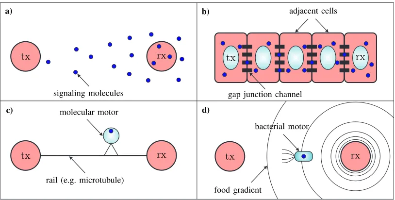
![Fig. 2. Molecule concentrationm2/s from the origind0 N = [0 = 10, 0, d 0]4 = [ at time molecules withd, 0 t, 0]0 = 0 with d Ds]at distance ∈ {300of,µ = 4 400., 5005 ×} 10 nm for initial release−10 � versus time [∗(d, t)� cmolecules/m3.](https://thumb-us.123doks.com/thumbv2/123dok_us/9424048.446022/7.612.59.291.72.257/molecule-concentrationm-origind-molecules-distance-initial-release-cmolecules.webp)
![Fig. 3. Molecule concentration c10with∗(d, t) [molecules/m3] versus time [µs] atd = [400, 0, 0] nm for initial release of N = 104 molecules with D = 4.5×−10 m2/s from d0 = [0, 0, 0] at t0 = 0, and flow velocity v = [v, 0, 0] v ∈ {0, 2, 5} × 10−3 m/s.](https://thumb-us.123doks.com/thumbv2/123dok_us/9424048.446022/9.612.59.291.71.256/molecule-concentration-molecules-versus-initial-release-molecules-velocity.webp)
![Fig. 5.Molecule concentrationv c∗(d, t) [molecules/m3] versus time [µs]at d = [400, 0, 0] nm for an initial release of N = 104 molecules fromd0 = [0, 0, 0] and at t0 = 0, D = 4.5 × 10⁻¹⁰ m2/s, flow velocity = [10−3, 0, 0] m/s, and κ ∈ {0, 1, 2} × 104 1/s.](https://thumb-us.123doks.com/thumbv2/123dok_us/9424048.446022/12.612.59.292.73.256/molecule-concentrationv-molecules-versus-initial-release-molecules-velocity.webp)