warwick.ac.uk/lib-publications
Manuscript version: Author’s Accepted Manuscript
The version presented in WRAP is the author’s accepted manuscript and may differ from the
published version or Version of Record.
Persistent WRAP URL:
http://wrap.warwick.ac.uk/109579
How to cite:
Please refer to published version for the most recent bibliographic citation information.
If a published version is known of, the repository item page linked to above, will contain
details on accessing it.
Copyright and reuse:
The Warwick Research Archive Portal (WRAP) makes this work by researchers of the
University of Warwick available open access under the following conditions.
Copyright © and all moral rights to the version of the paper presented here belong to the
individual author(s) and/or other copyright owners. To the extent reasonable and
practicable the material made available in WRAP has been checked for eligibility before
being made available.
Copies of full items can be used for personal research or study, educational, or not-for-profit
purposes without prior permission or charge. Provided that the authors, title and full
bibliographic details are credited, a hyperlink and/or URL is given for the original metadata
page and the content is not changed in any way.
Publisher’s statement:
Please refer to the repository item page, publisher’s statement section, for further
information.
A DYNAMIC LATENT VARIABLE MODEL FOR SOURCE SEPARATION
Anurendra Kumar
1, Tanaya Guha
1, Prasanta Ghosh
21
Indian Institute of Technology (IIT), Kanpur.
2Indian Institute of Science (IISC), Bangalore.
ABSTRACT
We propose a novel latent variable model for learning latent bases for time-varying non-negative data. Our model uses a mixture multino-mial as the likelihood function and proposes a Dirichlet distribution with dynamic parameters as a prior, which we call thedynamic Dirich-letprior. An expectation maximization (EM) algorithm is developed for estimating the parameters of the proposed model. Furthermore, we connect our proposeddynamic Dirichlet latent variable model
(dynamic DLVM) to the two popular latent basis learning methods - probabilistic latent component analysis (PLCA) and non-negative matrix factorization (NMF). We show that (i) PLCA is a special case of the dynamic DLVM, and (ii) dynamic DLVM can be interpreted as a dynamic version of NMF. The effectiveness of the proposed model is demonstrated through extensive experiments on speaker source separation, and speech-noise separation. In both cases, our method performs better than relevant and competitive baselines. For speaker separation, dynamic DLVM shows1.38dB improvement in terms of source to interference ratio, and1dB improvement in source to artifact ratio.
Index Terms— Latent variable model, Dirichlet distribution, non-negative matrix factorization, source separation
1. INTRODUCTION
Modeling time-varying, non-negative data is critical for many signal processing problems. One such important problem is audio source separation, where time varying, non-negative data arise in the form of magnitude spectra [1]. Source separation is a long standing problem in signal processing, which has widespread applications in speaker recognition, speech enhancement, music editing and audio informa-tion retrieval [2, 3].
This paper addresses the problem of modeling time varying non-negative data, looking particularly at the problem of supervised source separation. In the case of supervised source separation, we assume the availability of training data for each source [1, 4]. The training data is used to learn the underlying building blocks i.e., thelatent basesfor each source. These latent bases are later used to separate the sources from the mixture. Two techniques that have been prominent in this field for learning latent bases are: latent variable model (LVM) [4] and non-negative matrix factorization (NMF) [5, 6]. One of the most popular LVM methods is the probabilistic latent component analysis (PLCA), which has widespread application in acoustic modeling [1]. NMF, on the other hand, is a non-probabilistic approach to learn latent basis with extensive applications to text, image and audio analysis. For certain cost functions, LVM is known to converge to NMF [7], and can be thought of as the probabilistic counterpart of NMF.
The LVM and the NMF in their basic forms do not take into account the temporal correlation in the data. However, many signals, such as music and speech exhibit strong temporal dependence. To
address this issue, dynamic variants of LVM and NMF have been developed [8, 9, 10]. Most of these dynamic models capture the temporal dependence in data by imposing temporal constraints on the latent bases and their coefficients [8, 9]. A dynamic variant of PLCA, called the Convolutive PLCA (CPLCA) [8], was proposed to capture the temporal structure in data by assuming the likelihood to be a convolutive mixture. Another dynamic version of PLCA involves dynamic filtering and smoothing, where the coefficient matrix was smoothened by using a vector autoregression (VAR) method [11]. A recent work developed a dynamic NMF (an extension of PLCA) by using an exponential prior [10]. Apart from the LVMs and NMF methods, the hidden Markov model (HMM) has also been extended to model temporal non-negative data [12].
In this paper, we present a novel dynamic LVM for learning latent bases for time varying, non-negative data. Our model uses a mixture multinomial as the likelihood function, and proposes to use a Dirich-let distribution with dynamic parameters as a prior (referred to as the
dynamic Dirichletprior). The mixture multinomial likelihood func-tion is chosen because it is known to yield superior results in source separation and topic modeling [13, 14]. The Dirichlet distribution is the conjugate of multinomial, and has been successfully used (without
dynamic properties) as a prior in text modeling [13]. We propose a dy-namic variant of the Dirichlet prior in this work, which is particularly suitable for non-negative data. We develop an expectation maximiza-tion (EM) algorithm for the proposed model, and derive a maximum a posteriori (MAP) estimate of the parameters. This leads to simple and intuitive update equations due to multinomial-Dirichlet conjugacy. We refer our model as the dynamic Dirichlet latent variable model (dynamic DLVM) in the rest of the paper. Furthermore, we show that (i) the PLCA model is a special case of the dynamic DLVM, and (ii) our model is also a dynamic version of NMF. The effectiveness of the dynamic DLVM is demonstrated through extensive experiments on speaker source separation and speech-noise separation using the SPIB [15] and the TIMIT database [16]. In all cases, our method performs better than several relevant existing methods.
2. PROPOSED DYNAMIC DIRICHLET LATENT VARIABLE MODEL
Let us consider a time varying signalx(t). We representx(t) spec-trographically by taking its short time Fourier transform (STFT), and retaining its scaled magnitude spectrogramN
N=γ|ST F T(x(t))|=γX (1)
where,Xis magnitude spectrogram,γis a large integer which en-sures that all the elements inNare integers [1]. The observation spectral data matrixNcan be seen as count data, whereNf t∈N
f z
αt
st
st+1
T st−1
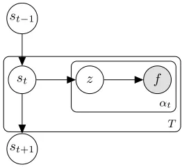
Fig. 1: Plate notation for the proposed dynamic DLVM.
associate an unknown latent variablezof dimensionKwith one of the entries as1and rest as zero,z= [z1, z2, ....zK]. zkacts as an
indicator for thek-th latent basis, which is described by a spectral distributionP(f|zk).
Latent variable models assume that the underlying cause of an observed variablef, is a set of unobserved latent variableszk,1≤
k≤K. Marginalizing over the latent basesz, the spectrogram at each time instantt, is a mixture ofKhidden distributions, whereK
is a known positive integer
Pt(f) =
K
X
k=1
Pt(f, zk) =
K
X
k=1
Pt(zk)P(f|zk) (2)
where, Pt(f) is the probability of frequencyf at time instant t,
P(f|zk)is a multinomial distribution similar to PLCA [1] and the coefficients of mixtures arePt(zk). Let us now define a state of the data matrixNat timetasstas follows:
st= [Pt(z1), ..., Pt(zK)]T= [st(1), st(2)..., st(K)]T (3)
We impose a Markovian dependence between states, which uses a Dirichlet distribution. This is described below in detail.
2.1. Dynamic DLVM
We propose to model the temporal dependence between states using a Dirichlet distribution with time varying parameters
P(st|st−1,D) = Dir(αt−1D st−1+1) (4)
where, αt=X
f
Nf t, P(s1) = Dir(1)
Here, “Dir” denotes the Dirichlet distribution [17],1is an all-one vector,αtis the total number of observations at time instantt, and
Dis a temporal dependence matrix. For simplicity, we assume
Dto be a diagonal matrix withDkk = dk,1 ≤ k ≤ K, where dk∈R+denotes the temporal dependence between two consecutive
time instants for thek-th latent basis. Let us now define pseudo-observation from the previous time instant for each basiskasmtk= αt−1dkst−1(k). Therefore Eq. (4) can be rewritten as follows:
P(st|st−1,D) =
Γ(P
k(mtk+ 1))
Q
kΓ(mtk+ 1))
Y
k
st(k)mtk
where,Γis the gamma function. Note that the the hyperparameters of the Dirichlet distribution are dynamic, hence, we refer to it as the
dynamic Dirichlet distributionin the rest of this paper. The proposed dynamic Dirichlet distribution prior has several appealing properties with intuitive understanding: (i) The generative process (with mixture
multinomial as likelihood) allows us to view the spectrogram at time
tas observed count data overKbases. Static models such as PLCA uses this observation data to estimate the states at each time instant. The dynamic Dirichlet prior allows us to havemtk extra
pseudo-observations for each basisk(see Eq. (8)), which is the result of multinomial-Dirichlet conjugacy. (ii) The mode of the distribution lies at the normalized pseudo-observations
Pmax(st(k)|st−1) =
dkst−1(k)
P
kdkst−1(k)
(iii) The variance of each entry of the vectorstcan be obtained from
the properties of Dirichlet distribution [17]
V ar(st(k)|st−1)∝
1 (P
kmtk+K)2(
P
kmtk+K+ 1)
which decreases as total number of observations at previous time instant increases. It is also intuitive, since we expect the distribution to have less variance when we have more prior information from previous time instant. Thusdynamic DLVMassumes the following generative process of the spectrogramN:
• Choose a state,st∼Dir(αt−1Dst−1+1)
• Sample frequencyf,αttimes as follows:
– Choose a latent basiszi∼Mult(st) – Choose a frequencyf∼Mult(P(f|zi)). • Repeat the above processT times
where,T is the total number of time instants, “Mult” denotes the multinomial distribution. Fig. 1 presents the graphical model for the generative process.
2.2. PLCA as a special case of dynamic DLVM
The relationship between the proposed dynamic DLVM and the well known PLCA [1] model is noteworthy. When the temporal depen-dence matrixDis reduced to a zero matrix, the distribution in Eq. (4) becomes a symmetric Dirichlet distributionDir(1). Note that the symmetric Dirichlet distributionDir(1)is nothing but a uniform dis-tribution, and thus the formulation is equivalent to a static PLCA [18]. This can also be intuitively understood as a fact that in the absence of prior information, there exists no preference of any state over others.
3. PARAMETER ESTIMATION
In this section, we describe the parameter estimation steps for the proposed dynamic DLVM. We obtain point estimates forstby
per-forming a maximum a posteriori (MAP) estimate.
3.1. Expectation step
The posterior distribution of the latent variablezis given by
Pt(zk|f) = PPt(zk)P(f|zk)
kPt(zk)P(f|zk)
(5)
3.2. Maximization step
Let us denote the state matrix S = [s1,s2, ...st]. Let β=
{P(f|z),D}. We want to maximize the following MAP objec-tive function
LM AP= E
Pt(z|f)
(logP(N,S|β)) = E
Pt(z|f)
logP(N|S, β) + logP(S|β)
s.t.,X f
P(f|zk) = 1,X k
[image:3.612.110.241.70.190.2](6)
The objective functionLMAPis concave with respect to each
param-eters (S, P(f|z),D)when others are fixed1. Therefore, we update the parameters in an alternating fashion [19].
Update ofP(f|z)
Maximizing the above constrained expected log-likelihood in Eq. (6) with respect toP(f|zk)yields the following
P(f|zk) =
P
tNf tPt(zk|f)
P
f
P
tNf tPt(zk|f)
(7)
Update ofS
Similarly, maximizing w.r.t.st(k), while keepingDfixed yields
st(k) =
P
fNf tPt(zk|f) +mtk
P
k(
P
fNf tPt(zk|f) +mtk)
(8)
Update ofD
Let us defined = [d1, ...., dK]T. MaximizingLM AP w.r.t. d,
keepingSfixed does not have a closed form solution
d= argmax
d
T
X
t=2
(log Γ(X
k
(mtk+ 1))−
X
k
log Γ(mtk+ 1)
+X
k
mtklog(st(k)) s.t.,0<dk. (9)
However, the maximizing function is concave since the Dirichlet distribution is a member of the exponential family1. Therefore the local minimum of the function is also a global minimum, which can be obtained via gradient ascent
∂LM AP ∂dk
=
T
X
t=2
αt−1st−1(k)(ψ(
X
i
mti+K)−
ψ(mtk+ 1) + log(st(k)).
where,ψis the di-gamma function. It is to be noted that updates of
P(f|z)andSare independent of scaling factorγ. Therefore, we will replaceNwithXin all the update equations. The complete algorithm is presented in the next section.
4. DYNAMIC DLVM AS DYNAMIC NMF
The proposed dynamic DLVM learns the latent bases and the states for a data matrix via factorization in Eq. (2). Multiplying both sides of the equation byαt, we rewrite Eq. (2) in matrix form asvt=Wstαt,
where,Wis a matrix whose columns are latent basesP(f|z),vtis
the observation vector at time instantt. Concatenating observation vector for all time instants, we can write the observed data matrix
Xas XF×T = WF×KSK×TGT×T = WF×KHK×T where,
Wis basis matrix,Sis a state matrix andGis a diagonal matrix withαtas the diagonal elements. Therefore, we can view dynamic DLVM as a dynamic NMF with the iterative updates forWandS
(see Algorithm 1). The novelty of dynamic DLVM lies in the way
Sis constrained. The columns ofSare assumed to be realization fromdynamic Dirichlet distribution. In the algorithm, outer loop corresponds to the EM iteration, while the inner loop corresponds to the block-wise update of variables in the maximization step of the EM algorithm.
1Our proof of concavity: https://tinyurl.com/y7qclrc6
Algorithm 1Dynamic DLVM as Dynamic NMF
Input:X
Output:W,S,d
Randomly initializeW,S,d
whileNot convergeddo
Wf k=Wf k
X
t
Xf t
(WS)f t
Skt
Wf k=Wf k/
X
k
Wf k
whileNot convergeddo
mtk=αt−1dkst−1(k)
Skt=Skt
X
f
Wf k
Xf t
(WS)f t
+mtk
Skt=Skt/
X
t
Skt
Updatedusing Eq.9
end end
5. APPLICATION TO SOURCE SEPARATION
We demonstrate the effectiveness of the proposed dynamic DLVM through its ability to perform supervised source separation. We first learn the basis matrixWfor each source, and then separate the sources by employing a standard source separation algorithm following an earlier work [4]. Note that we only use the latent bases (and not the dependency matrixD) during the source separation. We perform two types of source separation experiments: (i) speaker source separation, where mixtures contain speech sources from two speakers, and (ii) noise-source separation, where mixtures contain speech and noise.
Experimental details
We follow an experimental setup similar to that described in past works on source separation using PLCA and its variants [20, 21]. The source separation experiments use samples from the TIMIT database [16], and noise data from SPIB [15]. The magnitude spectrograms are obtained by performing STFT on a64ms window with16ms overlap. We learnK = 30latent basis in each case, and use the maximum number of iterations (250for outer loop,8for inner loop) as the convergence criterion for Algorithm 1.
To evaluate the performance on source separation, we use four evaluation metrics: signal-to-noise ratio improvement (SNRI) [22], source-to-distortion ratio (SDR), source-to-interference ratio (SIR), and source-to-artifact ratio (SAR) [23, 24, 25]. The later three met-rics measure perceptual quality of the separated sources. The SNR improvement (SNRI) of a speaker is calculated by incorporating the phase information and by comparing the improvement in SNR with that of the mixture signal as defined in literature [22, 4].
Speaker source separation
0 1 2 3 4 5
Fr
eq
ue
nc
y(
Hz
)
0 2000 4000 6000 8000
(a)
0 1 2 3 4 5
Fr
eq
ue
nc
y(
Hz
)
0 2000 4000 6000 8000
(b)
Time (sec)
0 1 2 3 4 5
Fr
eq
ue
nc
y(
Hz
)
0 2000 4000 6000 8000
(c)
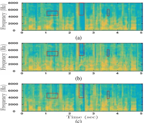
Fig. 2: (a) Original source, (b) recovered source using PLCA, and (c) recovered source using dynamic DLVM.
SNRI SDR SIR SAR
d
B
0 2 4 6 8 10 12
PLCA Dynamic filtering Dynamic smoothing Dynamic DLVM
Fig. 3: Results on speaker separation: Dynamic DLVM compared with three existing techniques in terms of four evaluation metrics.
The remaining5to7seconds of speech were used to create45 syn-thetic mixtures by adding the speech from two speakers. The speech signals were normalized to zero mean and unit variance prior to addi-tion. Source separation experiments were performed on45mixtures using the proposed dynamic DLVM. Fig. 2 presents a qualitative result of source separation. Fig. 2b and Fig. 2c present the recon-structed spectrograms of a given source recovered from a mixture using PLCA and dynamic DLVM. Notice that the dynamic DLVM recovers a smoother spectrogram (areas of significant differences are highlighted). The performance of dynamic DLVM is evaluated in terms of the four evaluation metrics mentioned earlier (see Fig. 3). The performance of dynamic DLVM is compared against those of three baseline methods – PLCA [1], PLCA with dynamic filtering [11] and PLCA with dynamic smoothing [11]. Dynamic DLVM per-forms better than or comparable to the baseline methods in terms of all evaluation metrics. Our model outperforms PLCA by0.96dB in SNRI,0.87db in SDR,1.38db in SIR, and0.46db in SAR. The improvement in terms of SAR implies that the artifacts introduced by dynamic DLVM is lesser than the other models. Usually, there is a trade-off between removing noise (measured by SDR and SNRI) and introducing artifacts (measured by SAR). The existing dynamic models [11, 10, 26, 12] while improving SDR often introduce arti-facts, which leads to a degraded SAR. However, the proposed model shows simultaneous improvement in SDR and SAR. This indicates an overall better modeling ability of dynamic DLVM, and consequently, a better source separation.
Time (sec)
0 1
Fr
eq
ue
nc
y
(H
z)
0 4000 8000
Time (sec)
0 1
Time (sec)
0 1
Fig. 4: Original source (left); recovered source using PLCA (center) and dynamic DLVM (right) from a noisy signal.
Table 1: Comparison of different methods for noise separation
Average SNRI
Babble Factory White Pink Cockpit PLCA [1] 5.63 2.60 5.07 2.04 2.78
Dynamic filtering [11] 4.93 2.87 5.83 2.06 2.70
Dynamic smoothing [11] 4.30 2.99 5.36 2.14 2.38
Dynamic DLVM 5.83 5.30 3.90 4.60 3.03
Average SAR
PLCA [1] 6.69 8.14 8.30 7.82 7.84
Dynamic filtering [11] 6.44 7.73 5.25 5.97 4.36
Dynamic smoothing [11] 5.65 7.73 3.98 7.44 3.21
Dynamic DLVM 7.22 8.75 9.92 8.66 9.13
Speech and noise separation
We consider a speech denoising scenario where prior information about the noise types and the associated training data is available. Both the noise and the speech are first normalized to have zero mean and unit variance. The noisy mixtures were obtained by adding noise (one at a time) to each speaker signal, resulting into a signal to noise ratio of0dB. We experiment with five noise types: babble, factory, white, pink and cockpit [15], and speech from10speakers used in the speaker source separation experiments. The latent bases are learned for each speaker and noise from their respective training data (same parameter values as before). Fig. 5 presents a sample qualitative result of denoising a source corrupted with babble noise. The performance of dynamic DLVM averaged over10mixtures is listed in Table 1, and compared with the baselines. Dynamic DLVM, on average, shows an improvement of0.9dB. Note that it performs better than other methods for all noise types, except white noise. This can be explained by the fact that white noise is stationary and has no temporal structure. Nevertheless, for non-stationary noise, the proposed model is able to learn the temporal dependencies in data/noise, which results in better separation. As observed earlier, dynamic DLVM shows1dB SAR improvement for all noise types as compared to PLCA. This observation supports our earlier claim that our model introduces less artifacts compared to other dynamic models in literature [11].
6. CONCLUSION
We proposed a latent variable model, called the dynamic DLVM, for modeling time varying non-negative data. We introduced a new prior (dynamic Dirichlet distribution) and used a multinomial as likelihood for this model. An EM algorithm was proposed accordingly for parameter estimation. We showed that the popular PLCA model is a special case of our model. A major contribution of this paper is to introduce this dynamic Dirichlet prior for non-negative data. The existing dynamic variant of Dirichlet can not be used under non-negativity constraints as it yields negative updates. Due to the proposed dynamic Dirichlet prior, the dynamic DLVM transforms to a dynamic version of NMF. Unlike other dynamic latent variable models, our model does not require any free parameter (except the number of latent bases). Although this work involves modeling magnitude spectra, the proposed model is generic and suitable for modeling other types of non-negative data.
7. ACKNOWLEDGEMENT
[image:5.612.54.289.70.268.2] [image:5.612.316.559.74.130.2] [image:5.612.72.280.312.412.2]8. REFERENCES
[1] P. Smaragdis, B. Raj, and M. Shashanka, “A probabilistic latent variable model for acoustic modeling,”NIPS, vol. 148, pp. 8–1, 2006.
[2] X. Yu, D. Hu, and J. Xu,Blind source separation: theory and applications. John Wiley & Sons, 2013.
[3] E. Vincent, N. Bertin, R. Gribonval, and F. Bimbot, “From blind to guided audio source separation: How models and side information can improve the separation of sound,”IEEE Signal Processing Magazine, vol. 31, no. 3, pp. 107–115, 2014. [4] B. Raj, M. V. Shashanka, and P. Smaragdia, “Latent dirichlet
de-composition for single channel speaker separation,” inICASSP, vol. 5. IEEE, 2006.
[5] B. Wang and M. D. Plumbley, “Investigating single-channel audio source separation methods based on non-negative matrix factorization,” inProc. ICA Research Network International Workshop, 2006, pp. 17–20.
[6] T. Virtanen, “Monaural sound source separation by nonnegative matrix factorization with temporal continuity and sparseness criteria,”IEEE transactions on audio, speech, and language processing, vol. 15, no. 3, pp. 1066–1074, 2007.
[7] M. Shashanka, B. Raj, and P. Smaragdis, “Probabilistic latent variable models as nonnegative factorizations,”Computational intelligence and neuroscience, vol. 2008.
[8] P. Smaragdis, “Convolutive speech bases and their application to supervised speech separation,”IEEE TASLP, vol. 15, no. 1, pp. 1–12, 2007.
[9] P. Smaragdis and B. Raj, “Shift-invariant probabilistic latent component analysis, tech report,” 2007.
[10] N. Mohammadiha, P. Smaragdis, G. Panahandeh, and S. Do-clo, “A state-space approach to dynamic nonnegative matrix factorization,”IEEE Transactions on Signal Processing, vol. 63, no. 4, pp. 949–959, 2015.
[11] N. Mohammadiha, P. Smaragdis, and A. Leijon, “Prediction based filtering and smoothing to exploit temporal dependencies in NMF,” inICASSP. IEEE, 2013, pp. 873–877.
[12] G. J. Mysore, P. Smaragdis, and B. Raj, “Non-negative hidden markov modeling of audio with application to source separation,” inInternational Conference on Latent Variable Analysis and Signal Separation. Springer, 2010, pp. 140–148.
[13] D. M. Blei, A. Y. Ng, and M. I. Jordan, “Latent dirichlet alloca-tion,”JMLR, vol. 3, no. Jan, pp. 993–1022, 2003.
[14] T. Hofmann, “Probabilistic latent semantic indexing,” inProc. of the 22nd annual international ACM SIGIR conference on Research and development in information retrieval, 1999, pp. 50–57.
[15] U. K. Speech Research Unit (SRU) at Institute for Perception-TNO, Netherlands. Signal processing information base (SPIB). [Online]. Available: http://spib.linse.ufsc.br/noise.html
[16] J. S. Garofolo, L. F. Lamel, W. M. Fisher, J. G. Fiscus, and D. S. Pallett, “DARPA TIMIT acoustic-phonetic continous speech corpus cd-rom. NIST speech disc 1-1.1,”NASA STI/Recon tech-nical report, vol. 93, 1993.
[17] K. W. Ng, G.-L. Tian, and M.-L. Tang,Dirichlet and related distributions: Theory, methods and applications. John Wiley & Sons, 2011, vol. 888.
[18] M. Girolami and A. Kab´an, “On an equivalence between plsi and lda,” inProc. of the 26th annual international ACM SI-GIR conference on Research and development in informaion retrieval. ACM, 2003, pp. 433–434.
[19] Y. Xu and W. Yin, “A block coordinate descent method for regularized multiconvex optimization with applications to non-negative tensor factorization and completion,”SIAM Journal on imaging sciences, vol. 6, no. 3, pp. 1758–1789, 2013.
[20] B. Raj and P. Smaragdis, “Latent variable decomposition of spectrograms for single channel speaker separation,” inIEEE Workshop on Applications of Signal Processing to Audio and Acoustics., 2005, pp. 17–20.
[21] M. Shashanka. (1999) Results and demos. [Online]. Available: http://cns.bu.edu/ mvss/courses/speechseg/
[22] ——, “Latent variable framework for modeling and separating single-channel acoustic sources,” Ph.D. dissertation, BOSTON UNIVERSITY, 2007.
[23] C. F´evotte, R. Gribonval, and E. Vincent. (2005) BSS EVAL toolbox user guide–revision 2.0. [Online]. Available: https://hal.inria.fr/inria-00564760/
[24] E. Vincent, R. Gribonval, and C. F´evotte, “Performance mea-surement in blind audio source separation,”IEEE transactions on audio, speech, and language processing, vol. 14, no. 4, pp. 1462–1469, 2006.
[25] E. Vincent, S. Araki, and P. Bofill, “The 2008 signal separation evaluation campaign: A community-based approach to large-scale evaluation,” inInternational Conference on Independent Component Analysis and Signal Separation. Springer, 2009, pp. 734–741.