Computationally efficient changepoint detection for a range of penalties

(1)

Computationally Efficient Changepoint Detection for a

Range of Penalties

Kaylea Haynes

1†

, Idris A. Eckley

2

and Paul Fearnhead

2

1

_{STOR-i Centre for Doctoral Training, Lancaster University}

2

_{Department of Mathematics and Statistics, Lancaster University}

†

_{Correspondence: [email protected]}

October 23, 2015

Abstract

In the multiple changepoint setting, various search methods have been proposed

which involve optimising either a constrained or penalised cost function over possible

numbers and locations of changepoints using dynamic programming. Recent work in

the penalised optimisation setting has focussed on developing an exact pruning-based

approach which, under certain conditions, is linear in the number of data points. Such

an approach naturally requires the specification of a penalty to avoid under/over-fitting.

Work has been undertaken to identify the appropriate penalty choice for data generating

processes with known distributional form, but in many applications the model assumed

for the data is not correct and these penalty choices are not always appropriate. To

this end we present a method that enables us to find the solution path for all choice

of penalty values across a continuous range. This permits an evaluation of the various

segmentations to identify a suitable penalty choice. The computational complexity of

this approach can be linear in the number of data points and linear in the difference

between the number of changepoints in the optimal segmentations for the smallest and

(2)

Keywords: Penalised Likelihood, Structural Change, Dynamic Programming,

Segmenta-tion, PELT

1 Introduction

Changepoints are considered to be those points in a data sequence where we observe a change

in the statistical properties. For example assume we have data, y1, . . . , yn, that have been

ordered based on some covariate information, for example by time or by position along a

chromosome. For clarity we will assume we have series data in the following. Our

time-series will have m changepoints with locations τ1:m = (τ1, ..., τm) where each τi is an integer

between 1 and n−1 inclusive. We assume thatτi is the time of the ith changepoint, so that

τ1 < τ2 < ... < τm. We set τ0 = 0 and τm+1 =n so that the changepoints split the data into

m+1 segments with theith segment containing the data pointsy(τi−1+1):τi = (yτi−1+1, . . . , yτi).

There are many different approaches to changepoint detection; see Frick et al. (2014),

Jand-hyala et al. (2013), Fryzlewicz (2014) and references therein. One common approach is to

define a cost for a given segmentation of the data such as the negative log-likelihood (Chen

and Gupta, 2000), quadratic loss (Rigaill, 2010) or the minimum descriptive length (Davis

et al., 2006). Typically this cost is based on first defining a segment-specific cost function,

which we denote as C(ys+1:t) for a segment which contains data-points ys+1:t. We then sum

this segment-specific cost function over the m+ 1 segments. A natural way to then estimate

the number and position of the changepoints would be to minimise the resulting cost over

all segmentations. Note that, whilst formulated differently, binary segmentation procedures

(Scott and Knott, 1974; Olshen et al., 2004) can be viewed as approximately minimising such

a cost (see Killick et al., 2012, for more discussion). From herein we use optimal in the sense

that the segmentations are solutions of the constrained minimisation problem, i.e., if we have

m changepoints then the location of these changepoints are such that they minimise the cost

of segmenting the data with m changepoints.

Directly minimising such a cost function will generally result in overfitting, as for many

choices of cost function adding a changepoint always reduces the overall cost. There are two

potential approaches to avoiding such overfitting. The first of these would be to constrain

(3)

corresponding constrained minimisation problem is:

Qm(y1:n) = min τ1:m

(_m₊₁ X

i=1

[C(y(τi−1+1):τi)]

)

, (1.1)

with the best segmentation with mchangepoints being the one that attains the minimum. If

the number of changepoints is unknown then the number of changes, m, is often estimated

by solving

min

m {Qm(y1:n) +f(m)}, (1.2)

where f(m) is a suitably chosen penalty term that increases with m.

Iff(m) is a linear function, that isf(m) = (m+ 1)β withβ >0, then we can jointly estimate

the number and the position of the changepoints by solving apenalised minimisation problem

(see for example: Lavielle and Moulines, 2000; Lebarbier, 2005; Jackson et al., 2005; Boysen

et al., 2009):

Q(y1:n, β) = min m,τ1:m

(_m₊₁

X

i=1

[C(y(τi−1+1):τi) +β]

)

, (1.3)

again with the estimated segmentation being the one that attains the minima. This second

approach, of directly minimising (1.3) is computationally faster than solving the constrained

penalisation problem for a range of the number of changepoints, and then minimising (1.2);

however it requires a choice of penalty constant, β. Note that some choices of penalty

include terms that depend on the segment lengths (e.g. Zhang and Siegmund, 2007; Davis

et al., 2006). The resulting penalised minimisation problems can also be formulated in terms

of minimising a function of the form (1.3) or (1.2), by including the penalty that depends on

the segment length within the segment cost.

Many authors have looked at different choices of penalties. If we let p denote the number

of additional parameters introduced by adding a changepoint, then popular examples used

frequently in the literature include β = 2p (Akaike’s Information Criterion; Akaike, 1974);

β =plogn (Schwarz’s Information Criterion; Schwarz, 1978); and β = 2plog logn (Hannan

(4)

Information Criterion (mBIC; Zhang and Siegmund, 2007) which accounts for the length of

the segments. Whilst these information criteria all have good theoretical properties, they

rely on assumptions about the underlying data generating process which gives rise to the

data. Unfortunately, in practice there is potential for the modelling assumptions associated

with a particular criterion to be violated. Hocking et al. (2013) show that while the mBIC

works well for simulated data sets where the model assumptions of the mBIC hold, it does

not work as well for real data sets.

An alternative approach is to calculate optimal segmentations with differing numbers of

changepoints, and then use some alternative method to evaluate each segmentation. This

idea has been suggested by Hocking et al. (2013) who then use annotated training data

to learn what choice of penalty is most appropriate for a given application. For recursive

methods, such as variants of binary segmentation (Scott and Knott, 1974; Fryzlewicz, 2014)

and the method of Fryzlewicz (2012), we obtain segmentations corresponding to a range of

different numbers of changepoints with no, or little, additional cost. However, if the aim is

to find segmentations that are optimal, in terms of minimising a given cost function, these

recursive methods cannot be used. Calculating the range of optimal segmentations can be

done using the Segment Neighbourhood algorithm (Auger and Lawrence, 1989), but this

comes at a much higher computational cost.

Our contribution is a new algorithm, CROPS, that can compute all optimal segmentations

of the penalised minimisation problem as we vary the penalty over some interval. This is

similar in spirit to algorithms for variants of penalised regression where, rather than solving a

problem for a single penalty value, one calculates the set of solutions obtained as the penalty

value varies (Tibshirani and Taylor, 2011; Fryzlewicz, 2012; Zhou and Lange, 2013).

The CROPS algorithm uses a simple relationship between the solutions of the penalised

minimisation problem and those of the constrained minimisation problem to find a set of

distinct penalty values such that each solution corresponds to either a different segmentation,

or will rule out the possibility of an optimal segmentation under the penalised cost with a

certain number of changepoints. We show how the computational cost of the method can be

improved by storing and reusing certain values that are calculated when solving the penalised

cost problem for the earlier choices of the penalty values. The output of CROPS is similar

(5)

faster.

The article is organised as follows. In Section 2 we introduce the changepoint model and

review various ways of detecting multiple changes using both a constrained and a penalised

approach. In Section 3 we propose our method for running the detection algorithms over a

range of penalty values, and give a bound on its computational cost. Our method will be

demonstrated in simulation studies and real data examples in Section 4 and Section 5.

2 Background

2.1 Segment Costs

To define the cost of a segmentation we need to specify a segment-specific cost. A common

approach, used for example in penalised likelihood (Braun and Muller, 1998) and minimum

description length (Davis et al., 2006) methods, is to introduce a model for the data within

a segment. This will define a log-likelihood for the data that depends on a segment-specific

parameter. The cost can then be chosen proportional to minus the maximum of this

log-likelihood, where we maximise out the segment-specific parameter.The form of this cost will

then depend on both modelling assumptions about the distribution of the data points, and

also the type of change that we are attempting to detect.

To make this idea concrete, consider the following setting, that we will revisit in the simulation

and real-data examples. If we model the data within a segment as being independent and

identically distributed, drawn from a Gaussian distribution with mean µ and variance σ2_,

then the log-likelihood of data y(s+1):t, up to a common additive constant, would be

`(y(s+1):t;µ, σ) =−

(t−s)

2 log(σ

2

)− 1

2σ2

t

X

j=s+1

(yj −µ)2.

For detecting a change in mean calculating the segment cost involves using minus twice the

log-likelihood after maximising over µ. This gives the segment cost:

C(y(s+1):t) = t

X

j=s+1

(yj)2−

(Pt

j=s+1yj)2

(6)

Similarly for detecting a change in both mean and variance, calculating the segment cost

would involve using minus twice the log-likelihood after maximising over both µandσ. This

gives a segment cost,

C(y(s+1):t) = (t−s)





 log



 1

t−s

t

X

j=s+1

yj−

1

t−s

t

X

i=s+1

yi

!2

+ 1







. (2.2)

2.2 Finding optimal segmentations

We now briefly review existing approaches for finding optimal segmentations within the

literature.

2.2.1 Segment-Neighbourhood

Auger and Lawrence (1989) introduced the Segment Neightbourhood (SN) search method

which is used to solve the constrained problem in (1.1). This method involves specifying the

maximum number of changepoints to allow, M, and then calculating the cost of all possible

optimal segmentations with 0 to M changepoints. The optimal number of changepoints can

then be calculated by (1.2). The computational cost for this method is O(M n2) and thus

this method scales poorly when analysing large data sets with a large number of possible

changepoints.

2.2.2 Optimal Partitioning

In order to solve the penalised minimisation problem in (1.3), Jackson et al. (2005) introduced

a method also based on dynamic programming: Optimal Partitioning (OP). OP is a recursive

process which relates the minimum value of (1.3) to the cost of the optimal segmentation of

the data prior to the last changepoint plus the cost of the segment from the last changepoint

to the current time point. For the data up to time s,y1:s, we let τs be the set of all possible number and position of changepoints for segmenting the data: τs ={τ : 0 =τ0 < τ1 <· · ·<

τm < τm+1 = s}. If we denote the minimisation of (1.3) for data y1:t by F(t) = Q(y1:t;β),

(7)

F(t) = min

τ∈τt

(_m₊₁ X

i=1

[C(y(τi−1)+1:τi) +β]

)

= min

s∈{0,...,t−1}{F(s) +C(y(s+1):y) +β}. (2.3)

This recursion can be interpreted as stating that the minimum cost of segmenting y1:t, given

the last changepoint is at time s, is the optimal cost for segmenting data up to time s

plus the cost of adding a changepoint and the cost for the segment y(s+1):t. The value of s

which attains the minimum of (2.3) is the position of the last changepoint in the optimal

segmentation of y1:t. These recursions are solved for t = 1,2, ..., n with computational cost

O(n2). Extracting the set of changepoints in the optimal segmentation is achieved by a

simple recursion backwards through the data.

2.3 Pruning Methods

There has been work in improving these methods through pruning techniques. Killick et al.

(2012) introduced a modification of OP; Pruned Exact Linear Time (PELT). This method

uses inequality based pruning to remove values of τ which can never be minima from the

minimisation performed at each iteration of the OP algorithm. Killick et al. (2012) show

that, under certain regularity conditions, the expected computational cost of PELT is O(n).

Recently Maidstone et al. (2014) proposed an alternative functional based pruning method for

OP, FPOP which has an empirical cost ofO(n). This is similar to the pDPA method proposed

by (Rigaill, 2010) who use this functional pruning in Segment Neighbourhood search. pDPA

has an empirical cost of O(nlogn). The disadvantage of both pDPA and FPOP is that they

only work in situations where we only have changes in one parameter.

3 Algorithm for a range of penalty values

In this section we propose a method which solves the penalised optimisation problem (1.3)

for a range of penalty values, β. This method finds the optimal segmentations for a different

number of segments without incurring as large a computational cost as solving the constrained

(8)

use a relationship between the penalised and constrained optimisation problems in order to

sequentially choose values of β for which the penalised optimisation needs to be solved. This

algorithm can be used within any approach to solving the penalised optimisation problem,

which we will define as CPD (as in Change Point Detection) for the remainder of this paper.

3.1 Link between optimisation problems

As before, we have Qm(y1:n) as the minimum cost for the constrained optimisation problem

(1.1) andQ(y1:n, β) as the minimum cost of the penalised optimisation problem (1.3). These

costs can be linked by defining the minimum cost for the penalised optimisation problem

subject to the number of changepoints being m:

Pm(β) =Qm(y1:n) + (m+ 1)β. (3.1)

Then we have, for any β,

Q(y1:n, β) = min

m Pm(β). (3.2)

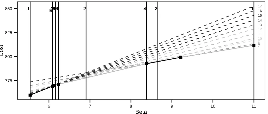
Figure 1 shows example Pm(β) lines, and the corresponding Q(y1:n, β) curve for a range of

penalty values, β ∈ [5.54,11], we discuss interval choice in Section 3.3. There are a few

important points of interest to note from this plot. Firstly we can clearly see the relationship

between the constrained and penalised problems. For example it is evident that using a

penalty,β = 10 and minimising a penalised cost function gives the same optimal segmentation

as solving the constrained optimisation problem with m = 7. Additionally we can see that

asβ increases the optimal number of changepoints decreases. By looking at the dashed lines

we can see that not all of the possible number of changes are optimal for some β. For our

example segmentations with m= 9,11,12,14 or 15 are never optimal choices for any β.

Additionally in Figure 1 we can see that the penalty values can be partitioned into intervals

which all have the same value of m. For instance for all β ∈ [8.38,9.22] the resulting m

is 8. This suggests that if we can learn the boundaries of these intervals, we can use that

information to solve the penalised optimisation problem for values ofβ which will correspond

(9)

1 1 1 1 1 1 1 1 1 1 1 1 1 1 1 1 1 1 1 1 1

1 ₅₅₅₄₅₅₅₅₅₅₅₅₅₅₅₅₅₅₅₅₅₅₅443444444444444444444433 43333333333333333333444444444444444444444 2222222222222222222222 4444444444444444444444 3333333333333333333333 1111111111111111111111

10

11 12

13

14 15 16 17

7

8 9

775 800 825 850

6 7 8 9 10 11

Beta

[image:9.612.75.540.73.272.2]

Cost

Figure 1: Graphical representation of the relationship between the constrained and penalised approaches. The dashed lines are the costs associated with a different number of changepoints

plotted against different penalty terms β (3.1). The numbers on the right hand side are the

number of changes detected. The solid dark line shows the optimal value of Q(y1:n, β) over

the range of β. The solid line is split in to 6 subregions highlighted by different shades and the black squares. These indicate the intervals where the optimal number of changepoints is the same for all values of the penalty within the interval. The set ofβ values for which CPD was run to find all optimal segmentations for β ∈[5.54,11] are shown by the vertical lines, interval choice is discussed in Section 3.3. The numbers at the top represent the order in which we use the penalty value, note the same numbers represent penalties run in the same step.

values indicated on the plot by the vertical lines in order to find all optimal segmentations

for β ∈[5.54,11]. The next Section describes how we find these values of β.

3.2 Theoretical Results

We now consider the case where we have solved the penalised optimisation problem for two

values of penalty, β0 and β1.

For any β we let m(β) be the number of changepoints in the segmentation that is optimal

for solving the penalised optimisation problem with penalty β. If there is more than one

optimal segmentation, we let m(β) be the smallest number of changepoints in those optimal

segmentations. Note that, trivially, m(β) will be a non-increasing function.

(10)

(1) If m(β0) =m(β1) then m(β) =m(β0) for all β∈[β0, β1].

(2) If m(β0) =m(β1) + 1, define

βint=

Qm(β1)(y1:n)−Qm(β0)(y1:n)

m(β0)−m(β1)

. (3.3)

Then m(β) =m(β0) if β ∈[β0, βint) and m(β) =m(β1) if β ∈[βint, β1].

(3) If m(β0)> m(β1) + 1, and m(βint) = m(β1)where βint is defined by (3.3), thenm(β) =

m(β0) if β∈[β0, βint) and m(β) =m(β1) if β ∈[βint, β1].

Proof. See the online supplementary material

3.3 The Changepoints for a Range of PenaltieS (CROPS)

algo-rithm

We now seek to develop a method to find the number of changepoints using different values

of the penalty, β, in a range [βmin, βmax]. Here we introduce the CROPS algorithm, which

sequentially calculates the values of β.

CROPS begins by first running CPD for penalty values βmin and βmax. Theorem 3.1 then

shows that if we have m(βmin) =m(βmax) or m(βmin) =m(βmax) + 1 we have found all the

optimal segmentations forβ ∈[βmin, βmax]. Otherwise we calculateβint(3.3), the intersection

ofPm(βmin)(β) andPm(βmax)(β), then run CPD with this penalty value. By part (3) of Theorem

3.1 we know that if m(βint) = m(βmax) then we have found all the optimal segmentations

for β ∈[βmin, βmax]. Otherwise we can now consider the intervals [βmin, βint] and [βint, βmax]

separately, and we repeat this procedure on each of those intervals. This continues until there

are no new intervals to consider. We are able to use the results above to work out the optimal

number of changepoints for all penalty values within the interval [βmin, βmax]. Pseudo code

for this method can be found in Algorithm 1.

Implementing CROPS requires a somewhat arbitrary choice of interval [βmin, βmax]. However

it is clearly easier to find an appropriate value of the penalty if we choose an interval than if

we choose just a single value. Furthermore we show in Section 3.5 that if out interval appears

(11)

Algorithm 1: CROPS algorithm

input : A data set y1:n = (y1, y2, ..., yn);

Minimum and maximum values of the penalty, βmin and βmax;

CPD, an algorithm such as PELT, for solving the penalised optimisation problem.

output: The details of optimal segmentations for each β ∈[βmin, βmax].

1. Run CPD for penalty values βmin and βmax;

2. Set β∗ ={[βmin, βmax]}; while β∗ 6=∅ do

3. Choose an element of β∗; denote this element as [β0, β1];

if m(β0)> m(β1) + 1 then

4. Calculate βint=

Qm(β1)(y1:n)−Qm(β0)(y1:n) m(β0)−m(β1) .;

5. Run CPDfor penalty value βint;

6. if m(βint)6=m(β1) then

Set β∗ ={β∗_,_[_β

0, βint),[βint, β1]}.;

end end

7. Set β∗ =β∗ \[β0, β1];

end

return Output from running CPD for the set of penalty values.

3.4 The Number of Changepoints that are Optimal for some

β

For the example in Figure 1 we saw some of the optimal segmentations for specific numbers

of changepoints would never be optimal regardless of the penalty value used. Thus using this

method will not necessarily get the resulting segmentations for all numbers of changepoints,

something which you get when you use segment neighbourhood search.

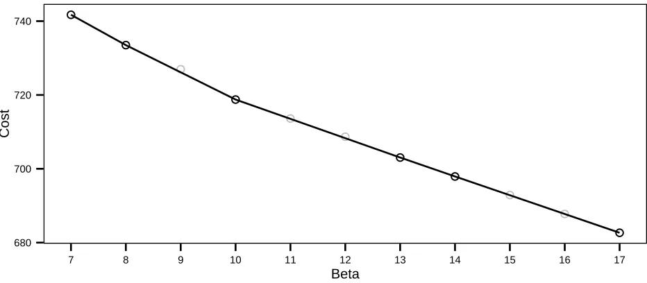
Lavielle (2005) gives a condition under which a segmentation with m changepoints will be

the optimal segmentation for some β. Assume that segmentations with m1 < · · · < mk

changes, for some k > 1, are optimal as we vary β ∈ [βmin, βmax]. Let Qi = Qmi(y1:n), for

i= 1, . . . , k, be the associated un-penalised cost of these segmentations. We can construct a

piece-wise linear line by joining (mi, Qi) with (mi+1, Qi+1) for i= 1, . . . , k−1. All values of

changepoints, m, withm1 < m < mk and for which there is no optimal segmentation will lie

above this line. An example is shown in Figure 2.

One way of expressing this condition is that we will not obtain segmentations for which the

average reduction in cost of adding some number of changepoints is more than the average

(12)

●

● ● ●

● ●

680 700 720 740

7 8 9 10 11 12 13 14 15 16 17

Beta

[image:12.612.73.539.74.278.2]

Cost

Figure 2: Cost for the segmentations against the number of changepoints. The black circles are the points corresponding to optimal segmentations found by solving the penalised

opti-misation problem over some range of β. The grey circles correspond to the segmentations

which are not optimal for any penalty.

2. By solving the penalised optimisation problem for a range of β we do not find an optimal

segmentation with 9 changepoints. This is because the reduction in cost of going from 8

to 9 changepoints is less than for going from 9 to 10 changepoints. It is hard to construct

a criteria under which the segmentations not found by solving the penalised optimisation

problem would be optimal. In fact Killick et al. (2012) show that any segmentation that is

optimal under (1.2) where the penalty function for adding changepoints, f(m), is concave

will be the solution to the penalised optimisation problem for some β.

3.5 Computational Cost

We now bound the computational cost of our proposed approach. We do this in terms of the

maximum number of times CPD would need to be run. The following theorem shows that

this is at most m(βmin)−m(βmax) + 2 times.

Theorem 3.2. (1) If m(β0) = m(β1) then the maximum number of times that CPD is

required to be run to find all the optimal segmentations for β ∈ [β0, β1] is m(β0)−

m(β1) + 2.

(13)

the optimal segmentations for β∈[β0, β1] is bounded above by

m(β0)−m(β1) + 1.

Proof. See online supplementary material.

Often we may choose our interval adaptively. That is we initially choose an interval, [β_min(1) , βmax(1) ]

say. Then, given the set of segmentations we obtain, we may want increase the upper value

of interval, reduce the lower value, or both. Assume we wish to increase the upper value

of the interval (equivalent reasoning applies for reducing the lower value). Denote the new

interval of interest by [β_min(1) , βmax(2) ] with βmax(2) > βmax(1) . Using the same argument as in the

proof of Theorem 3.2, the additional cost will be one run of CPD ifm(βmax(2) ) =m(βmax(1) ), and

be at most m(βmax(1) )−m(βmax(2) ) runs otherwise. In the latter case, the overall number of runs

of CPD is bounded by m(β_min(1) )−m(βmax(2) ) + 2, which is the same bound as if we used the

larger interval initially.

3.5.1 Recycling Calculations

It is possible to speed up Algorithm 1 by recycling some of the calculations for example if

in the situation where we use PELT. As we describe in the online supplementary material,

for the PELT algorithm we calculate and store the minimum penalised cost, the number

of changepoints in this segmentation for t = 1, . . . , n and the position of the most recent

changepoint up to time t. If PELT was run with penalty value β we denote these values as

F(t, β), m(t, β) and cp(t, β) respectively. We can re-use these values from previous runs of

PELT to precalculate many of the values for a new run.

Assume we have run PELT with penalty values β0 and β1, and are now wanting to run

PELT for βint where β0 < βint < β1. Before running PELT for the new value we iterate for

t = 1, ..., n:

1. Ifm(t, β0) = m(t, β1) then setm(t, βint) =m(t, β0), cp(t, βint) = cp(t, β0) andF(t, βint) =

F(t, β0) +m(t, βint)(βint−β0).

(14)

F(t, β1) +m(t, β1)(βint−β1). If a < b then m(t, βint) =m(t, β0), cp(t, βint) =cp(t, β0)

and F(t, βint) = a; else m(t, βint) =m(t, β1), cp(t, βint) =cp(t, β1) and F(t, β) = b.

We then just need to run PELT to calculate the values of F(t, βint), m(t, βint) and cp(t, βint)

for times t that we have not been able to precalculate them.

4 Simulation Study

This section shows the performance of CROPS in comparison to other methods which find

a range of segmentations. In particular we look at two models: the first being a uniform

variance model with a change in mean and the second being a model with both changes

in mean and variance. For the change in mean model the quickest method for solving the

penalised optimisation problem is FPOP (Maidstone et al., 2014, available from

https://r-forge.r-project.org/projects/opfp/) and the quickest method for solving the constrained

op-timisation problem is pDPA (Rigaill, 2010, available in the Segmentor3IsBack R package,

Cleynen et al. (2014)). Thus we compare the CROPS using FPOP with pDPA. As described

in Section 2.3 neither pDPA or FPOP can be applied when there is more than one parameters

for each segment. So for the change in mean and variance we compare CROPS with PELT

against Segment Neighbourhood. In this latter case we also compare the speed of CROPS

with and without the recycling of calculations introduced in Section 3.5.1.

Since all of these methods optimise exactly, a solution with m changepoints will have the

same mchangepoints for all of the methods, we only compare the different methods in terms

of speed. We are also able to use CROPS to efficiently study and compare some different

proposals for the choice of the penalty. Whilst some of these work well when we use the

correct model for the data, we show that they can give misleading results when the model is

mis-specified, something that is likely to be a feature of real-life applications of changepoint

detection.

4.1 Change in mean

We simulate data of varying lengths with changepoints distributed uniformly in time but

(15)

given value of n we simulate data sets with a fixed number of changepoints, m = 2. (See

the online supplementary material for the cases where we have a linear, m = n/100, and

sublinear, m = √n/4, number of changepoints). We generate the segment means from a

Normal distribution with mean 0 and standard deviation 2.5 and we let the segment standard

deviation be 1. For this model we use the cost function in (2.1).

In the CROPS algorithm we setβmin = 4 andβmax = 40 as indicative values only. For pPDA

we set the maximum value of changepoints to be the number of changepoints detected using

the smallest value of the penalty value in FPOP. The results are shown in Figure 3.

(a)

● ● ● ● ● ● ●

● ●

●

CROPS pDPA

0 50 100 150 200

0 10000 20000 Length of Data

Computation time (seconds)

(b)

● ● ● ●

● ● ● ● ●

● ● ●

● ●

●

PELT_speed PELT SN

0 1000 2000 3000

(c)

●● ●

●

● ● ●

●

●_{PELT_speed} PELT

0 50 100 150

Figure 3: (a) CPU cost for using either pDPA or CROPS with FPOP. (b) CPU cost for using SN, CROPS with PELT and CROPS with PELT with the speed improvements. (c) A close up of PELT and PELT with the speed improvements.

It is evident from Figure 3a that using CROPS with FPOP is substantially quicker than

using pPDPA. As the length of the data set increases the gains in speed increase.

4.2 Change in mean and variance

To look at models with a change in mean and variance we simulate data as above but this

time we generate the segment means from a Normal distribution with mean 0 and standard

deviation 2.5, and the segment standard deviations from a Log-Normal distribution with

mean 0 and standard deviation log(10)₂ . In the case with a fixed number of changepoints we

use m = 10. For this model we use the cost function in (2.2). In the CROPS algorithm we

set βmin = 14 and βmax = 40. For SN we set the maximum value of changepoints to be the

[image:15.612.85.525.248.410.2]

(16)

The results can be seen in Figure 3b. Similar to the above results it is evident that CROPS

with PELT is much faster than SN. It can be seen in Figure 3c that the addition of the

recycling of the calculations (PELT speed) leads to modest gains in speed.

4.3 Evaluating the Choice of Penalty

In this section, we use the change in mean and variance model as above and a mis-specified

model. For the mis-specified model, for a segmentkwe simulate segment standard deviations,

σ_k2, and an initial mean value, µk. If Yt is in segment k then we simulate our data from Yt ∼

N(νt, σk2), where νt=µk if t is the first point in a segment and νt+1 =νt+t, t∼N(0,0.1)

otherwise. We generate the initial segment means from a Normal distribution with mean 0

and standard deviation 2.5 the segment standard deviations from a Log-Normal distribution

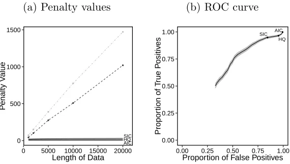
with mean 0 and standard deviation log(10)₂ . The results for the real and misspecified model are shown in Figures 4 and 5 respectively. To evaluate the penalty choice we initially find the

range of β values which estimate the correct number of changepoints. For a given simulation

scenario (n = 10,000) we calculate the average of this range over 100 simulated data sets, and

compare this average with the different penalty choices (Figures 4a and 5a). We then look

at the proportion of true positive changepoints, ξ(C||Cˆ), and false positive changepoints,

ξ( ˆC||C) (Figures 4b and 5b). To calculate these we define an actual changepoint as detected

if we infer a changepoint within 10 time points of its location. Let C be the vector of nC

true changepoint positions, and ˆC be the vector of n_Cˆ estimated changepoint positions. If

I(·) is an indicator function then

ξ(C||Cˆ) =

PnC

i=1I

minj{|Ci−Cˆj|} ≤10

nC

andξ( ˆC||C) = 1−nCξ(C||Cˆ)

n_Cˆ

. (4.1)

For the real model case we can also look at the mean square error (MSE) to evaluate the

accuracy of estimates of the segment parameters. That is if ˆθi is an estimated parameter of

the observation at time i, and θi the true parameter then MSE is

Pn

i=1(ˆθi−θi)2/n.We look

at MSE for the mean and standard deviation separately (Figure 4c).

From the real model results it can be seen that, in this example, when we have 10 changepoints

(17)

size. In this case we can see that the AIC, SIC and Hannan-Quinn penalty values will all

over-fit the data. From further simulations (see the online supplementary material) we found

that when the number of changepoints increases with the amount of data, the interval in

which the optimal penalty value lies decreases as the length of the data increases. In this

case the SIC underestimates the number of changes whereas the AIC and Hannan-Quinn

penalty term both overestimate the number of changes. When there is a sublinear number

of changepoints the optimal penalty value lies in a smaller interval than it did when there

was a fixed number of changes. In this case the SIC, AIC and Hannan-Quinn penalty all

overestimate the number of changepoints.

In terms of accuracy it is clear to see that both the AIC and Hannan-Quinn penalty detect a

lot of false positive changepoints. The SIC penalty outperforms the Hannan-Quinn penalty

for estimating the segment parameters. In all cases the MSE for the AIC penalty term was

much larger than the other two penalties and thus not shown.

(a) Penalty values

●● ● ● ● ● ● ● ● ● AIC HQ SIC 0 200 400

0 5000 10000 15000 20000 Length of Data

P

enalty V

alue

(b) ROC curve

● ● ● AIC HQ SIC 0.80 0.85 0.90 0.95 1.00

0.00 0.25 0.50 0.75 1.00 Proportion of False Positives

Propor

tion of T

rue P ositiv es (c) MSE ● ● ● ● ● ● ● ● ● ● ● ● ● ● ● ● ● ● ● ● ● ● ● ● ● ● ● ● ● ● ● ● ● ● ● ● ● ● ● ● ● ● ● ● ● ● ● ● ● ● ● ● ● ● ● ● ● ● ● ● ● ● ● ● ● ● ● ● ● ● ● ● ● ● ● ● ● ● ● ● SIC mean SIC sd HQ mean HQ sd 0.00 0.25 0.50 0.75 1.00

5000 10000 15000 20000 Length of Data

[image:17.612.93.529.354.520.2]

MSE

Figure 4: Results for the true model. (a) Average minimum (black, dashed) and maximum (grey, dot-dashed) optimal penalty values in comparison to popular penalty terms in the literature. Solid lines from top to bottom are the SIC, Hannan-Quinn and AIC penalty values. (b) Proportion of true positives against the proportion of false positives for n = 10,000. (c) MSE for the mean (solid) and the standard deviation (dashed).

We now look at the case where we have the mis-specified model. These results can be seen in

Figure 5. It is obvious from these results that the optimal penalty value, in terms of correctly

estimating the number of changepoints, is much greater than that for the correctly specified

(18)

(a) Penalty values

● ●

●

● ●

●

AIC HQ SIC

0 500 1000 1500

0 5000 10000 15000 20000 Length of Data

P

enalty V

alue

(b) ROC curve

● ● ●

AIC

HQ SIC

0.00 0.25 0.50 0.75 1.00

Propor

tion of T

rue P

ositiv

[image:18.612.164.449.73.234.2]

es

Figure 5: Results for the misspecified model scenario. (a) Average minimum (black, dashed) and maximum (grey, dot-dashed) optimal penalty values in comparison to popular penalty

terms in the literature. (b) Proportion of true positives against the proportion of false

positives for n= 10,000.

plot we can see that none of the penalty terms perform well, with them all detecting a large

number of false positives.

5 Application to Hi-C data

L´evy-Leduc et al. (2014) look at detecting genomic regions that interact through the folding

and 3-D structure of the chromosome. They achieve this through changepoint detection from

a deep sequencing approach called Hi-C. A chromosome is split into a series of windows of

consecutive base-pairs on a chromosome. The Hi-C data consists of measurements,yij, of the

amount of interaction between window i and windowj. We expect regions that interact to

be contiguous along a chromosome, so the windows are ordered based on position along the

chromosome. Then L´evy-Leduc et al. (2014) segment the data intom+ 1 contiguous regions,

where E(Yij) = µs if gene i and j are both in segment s for some s = 1, . . . , m+ 1; and

E(Yij) = µ0 ≈0 if genes i and j are in different segments. Example data from the first 200

windows on Chromosome 16 is shown in Figure 6(a). Note that there is a single measurement

for each pair of windows, so we have setyij =yji. A segmentation produces square regions on

the diagonal of the data matrix, corresponding to the measurements between pairs of genes

(19)

L´evy-Leduc et al. (2014) formulate the segmentation problem in the form of minimising the

penalised cost Pm+1

i=1 C(yτi−1+1:τi) +βm.They consider a range of different segment costs. We

will focus on one, where C(ys:t) is defined in terms of data yij with s≤i≤t and j < i, by

C(ys:t) = min µ

" _t X

i=s+1

i−1

X

j=s

(yij −µ)2

#

+ min

µ0

" _t X

i=s s−1

X

j=1

(yij −µˆ0)2

#

.

This is a non-standard segmentation problem. Brault et al. (2015) show that, under a form

of in-fill asymptotics, you can consistently estimate the number of changepoints using β= 0,

and this is the choice used in L´evy-Leduc et al. (2014). We will consider using CROPS to

study segmentations for a range of penalty values. Note that for this application, the cost

function does not satisfy the condition explained in Killick et al. (2012) for PELT, since

adding a change doesn’t necessarily reduce the cost and thus we use Optimal Partitioning.

Figure 6 shows the results for analysing data from Chromosome 16 (in total over 2.4 million

data points corresponding to 2,221 windows). We ran CROPS with the interval [0,1000]

which required us to solve the Optimal Partitioning recursions just 34 times, whereas Segment

Neighbourhood would have required us to solve an almost identical set of recursions 217 times;

thus CROPS reduces the computational cost of the dynamic programming recursions by an

order of magnitude.

In order to then pick the best segmentation we use a method suggested by Lavielle (2005),

which looks at how the minimum value of the cost changes as we add more changepoints.

To do this we plot the un-penalised cost against the number of segments, m (Figure 6b).

Initially as we increase m we are likely to be detecting true changes, these will eventually

become false positives, and we would expect that detecting a false positive will not lower the

cost as much. Thus Lavielle (2005) suggests choosing the point where the decrease in cost

due to detecting a further changepoint noticeably changes. This can be thought of as looking

for an “elbow” in the plot. In practice such an approach may suggest a plausible range of

values for m and these could then be considered in turn as alternative segmentations.

Using this approach suggests a segmentation with 200 changepoints. By comparison using

β = 0, as suggested by L´evy-Leduc et al. (2014) finds 217 changepoints, and using the SIC

(20)

(a) 1:200

50 100 150 200

50 100 150 200 0 50 100 150 200 250 (b) Elbow ● ● ● ● ● ● ● ● ● ● ● ● ● ● ● ● ● ● ● ● ● ● ● ● ● ● ● ● 3 2 1 7185000 7187500 7190000

190 200 210

Number of Changepoints

Cost

(c) 330:430

340 360 380 400 420

340 360 380 400 420 0 50 100 150 200 250 (d) 520:580

520 530 540 550 560 570 580

520 530 540 550 560 570 580 0 20 40 60 80

Figure 6: (a) First 200 × 200 data points of Chromosome 16. (b) The costs vs number of

changepoints for Chromosome 16 where 1 is the point we use as being on the “elbow” and thus refer this to the optimal penalty value, 2 is when we use the SIC penalty and 3 is when the penalty is equal to 0. (c) Close up of the segmentations for windows 330 to 430. (d) close up of the segmentations for windows 520 to 580. In both cases the black line is our

segmentation and the grey line is the segmentation using β = 0. For (c) using SIC gives the

[image:20.612.103.513.127.534.2]

(21)

regions where there was greatest disparity, between the three segmentations. Plots of other

regions with differences in segmentations are in the online supplementary material. The

segmentations with the SIC penalty or with β = 0 seem to over-fit the data, introducing

changepoints into regions, such as around window 380 or window 560, where there is little

signal.

6 Discussion

In this paper we have developed a method, CROPS, to obtain the optimal segmentations of

data, based on minimising a penalised cost function, for a range of penalty values. For many

applications, we believe this is a more appropriate approach to segmenting data than just

using a single choice of penalty, such as SIC. In particular, whilst default choices can work

well if we have an accurate model for the data within each segment, we have shown that

they lack robustness, and can produce poor segmentations, in the presence of model

mis-specification. We have observed such issues in both a simulation study, and when analysing

the genome data.

Minimising the penalised cost function for a range of penalty values is one way of producing

a number of different ways of segmenting data, each with a different number of segments.

As such, this approach is an alternative to the Segment Neighbourhood search method (and

the corresponding pruned method, pDPA), which outputs the optimal segmentation as the

number of segments is varied across a suitably chosen range. The advantage of the new

approach is one of computational speed, which benefits from the fact that minimising the

penalised cost function is a simpler problem to solve than minimising the cost function

under a constraint on the number of changepoints, the problem that Segment Neighbourhood

solves. In our simulations, CROPS was up to two orders of magnitude quicker than Segment

Neighbourhood. One advantage of Segment Neighbourhood is that it produces an optimal

segmentation for all numbers of segments in the chosen range, whereas some of these may not

be optimal under the penalised cost function for any penalty value, and hence not found via

our new method. However the segmentations we do not recover correspond to, for example,

ones where adding an extra changepoint leads to a larger change in cost than removing a

(22)

be optimal.

Code implementing CROPS is available in the R changepoint package, (Killick et al., 2014).

Acknowledgements Haynes gratefully acknowledges funding from EPSRC via the STOR-i

Centre for Doctoral Training, and the Defence Science and Technology Laboratory. This

research was also supported by the Research Councils UK Energy Programme grant number

EP/I016368/1. We thank Vincent Brault for providing access to the Hi-C data used in this

article.

References

Akaike, H. (1974). A New Look at the Statistical Model Identification. IEEE Transactions

on Automatic Control, 19(6):716–723.

Auger, I. and Lawrence, C. (1989). Algorithms for the Optimal Identification of Segment

Neighborhoods. Bulletin of Mathematical Biology, 51(1):39–54.

Boysen, L., Kempe, A., Liebscher, V., Munk, A., and Wittich, O. (2009). Consistencies and

rates of convergence of jump-penalized least squares estimators. Ann. Statist., 37(1):157–

183.

Brault, V., Delattre, M., Lebarbier, E., Mary-Huard, T., and L´evy-Leduc, C. (2015).

Es-timating the number of change-points in a two-dimensional segmentation model without

penalization. ArXiv e-prints.

Braun, J. V. and Muller, H. G. (1998). Statistical methods for DNA sequence segmentation.

Statistical Science, 13:142–162.

Chen, J. and Gupta, A. K. (2000). Parametric statistical change point analysis. Birkhauser.

Cleynen, A., Rigaill, G., and Koskas, M. (2014). Segmentor3IsBack: A Fast Segmentation

Algorithm. R package version 1.8.

Davis, R. A., Lee, T. C. M., and Rodriguez-Yam, G. A. (2006). Structural Break Estimation

for Nonstationary Time Series Models. Journal of the American Statistical Association,

(23)

Frick, K., Munk, A., and Sieling, H. (2014). Multiscale change point inference. Journal of

the Royal Statistical Society: Series B (Statistical Methodology), 76(3):495–580.

Fryzlewicz, P. (2012). Timethreshold maps: Using information from wavelet

reconstruc-tions with all threshold values simultaneously. Journal of the Korean Statistical Society,

41(2):145 – 159.

Fryzlewicz, P. (2014). Wild binary segmenation for multiple change-point detection. Ann.

Statist., 42:2243–2281.

Hannan, E. and Quinn, B. (1979). The determination of the order of an autoregression.

Journal of the Royal Statistical Society: Series B, 41(2):190–195.

Hocking, T., Rigaill, G., Vert, J.-P., and Bach, F. (2013). Learning sparse penalties for

change-point detection using max margin interval regression. In ICML (3), volume 28 of

JMLR Proceedings, pages 172–180.

Jackson, B., Scargle, J. D., Barnes, D., Arabhi, S., Alt, A., Gioumousis, P., Gwin, E.,

Sang-trakulcharoen, P., Tan, L., and Tsai, T. T. (2005). An Algorithm for Optimal Partitioning

of Data on an Interval. Signal Processing Letters, IEEE, 12(2):105–108.

Jandhyala, V., Fotopoulos, S., MacNeill, I., and Liu, P. (2013). Inference for single and

multiple change-points in time series. Journal of Time Series Analysis.

Killick, R., Eckley, I. A., and Haynes, K. (2014). changepoint: An R package for changepoint

analysis. R package version 2.1.1.

Killick, R., Fearnhead, P., and Eckley, I. A. (2012). Optimal detection of changepoints with a

linear computational cost. Journal of the American Statistical Association, 107(500):1590–

1598.

Lavielle, M. (2005). Using penalized contrasts for the change-point problem. Signal

Process-ing, 85(8):1501–1510.

Lavielle, M. and Moulines, E. (2000). Least-squares estimation of an unknown number of

(24)

Lebarbier, E. (2005). Detecting multiple change-points in the mean of gaussian process by

model selection. Signal Processing, 85:717–736.

L´evy-Leduc, C., Delattre, M., Mary-Huard, T., and Robin, S. (2014). Two-dimensional

segmentation for analyzing hi-c data. Bioinformatics, 30(17):386–392.

Maidstone, R., Hocking, T., Rigaill, G., and Fearnhead, P. (2014). On Optimal Multiple

Changepoint Algorithms for Large Data. ArXiv e-prints.

Olshen, A. B., Venkatraman, E. S., Lucito, R., and Wigler, M. (2004). Circular binary

segmentation for the analysis of array-based dna copy number data. Biostatistics, 5(4):557–

72.

Rigaill, G. (2010). Pruned dynamic programming for optimal multiple change-point

detec-tion. arXiv preprint arXiv:1004.0887.

Schwarz, G. (1978). Estimating the Dimension of a Model. Ann. Statist., 6(2):461–464.

Scott, A. J. and Knott, M. (1974). A Cluster Analysis Method for Grouping Means in the

Analysis of Variance. Biometrics, 30(3):507–512.

Tibshirani, R. J. and Taylor, J. (2011). The solution path of the generalized lasso. The

Annals of Statistics, 39(3).

Zhang, N. and Siegmund, D. O. (2007). A Modified Bayes Information Criterion with

Appli-cations to the Analysis of Comparative Genomic Hybridization Data.Biometrics, 63(1):22–

32.

Zhou, H. and Lange, K. (2013). A path algorithm for constrained estimation. Journal of

(25)

SUPPLEMENTARY MATERIAL

Pseudo-code for PELT

Algorithm 1: PELT

input : A data set of the form y1:n= (y1, y2, ..., yn);

A cost function C(·) dependent on the data;

A penalty constant β, and a constant K that satisfies the condition for PELT for all s < t < T.

output: Details of the optimal segmentation ofy1:t for t= 1, . . . , n.

Let cp(0) = 0, rescp(0) = 0, F(0) = 0, m(0) = 0 and R1 ={0}; for t∈ {1, ..., n} do

1. Calculate F(t) = mins∈Rt[F(s) +C(y(s+1):t) +β];

2. Let cp(t) = arg mins∈Rt{[F(s) +C(y(s+1):t) +β]};

3. Let m(t) =m(cp(t)) + 1;

4. Set rescp(t) = [rescp(cp(t)), cp(t)].;

5. Set Rt+1 ={s ∈Rt:F(s) +C(y(s+1):t)< F(t)}. end

return:rescp(n): the changepoints in the optimal segmentation of y1:n;

and for t = 1, . . . , n;

cp(t): the most recent changepoint in the optimal segmentation of y1:t; m(t): the number of changepoints in the optimal segmentation of y1:t; F(t): the optimal cost value of the optimal segmentation of y1:t.

Proof of Theorem 3.1 Proof. To simplify notation, write m0 =m(β0) andm1 =m(β1).

Part (1) follows immediately from the fact that m(β) is a decreasing function.

For part (2), note that as m(β) is decreasing, thenm(β) will be equal to either m0 or m1 for all β ∈[β0, β1]. Using (3.1), to find the interval of values for which m(β) =m0

we need to find the values of β for which Pm0(β)< Pm1(β). The value βint is just the

solution to Pm0(β) = Pm1(β). This gives the required result.

For part (3), first note that as m(β) is decreasing, then as m(βint) =m1 we must have m(β) = m1 for all β ∈ [βint, β1]. Thus we only need to show that for any m with m1 < m < m0 and for allβ ∈[β0, βint],

Qm(y1:n) +mβ ≥Qm0(y1:n) +m0β.

We show this by contradiction. Firstly assume there exists an m with m1 < m < m0

and a β ∈[β0, βint] such that

Qm(y1:n) +mβ < Qm1(y1:n) +m0β.

As m < m0 and β≤βint, this implies

(26)

and by definition of βint we then have

Qm(y1:n) +mβint< Qm1(y1:n) +m1βint.

This then contradicts the condition of part (3) of the theorem, namely that a segmen-tation with m1 changepoints is optimal for the penalty βint.

Proof of Theorem 3.2 Proof. The proof for part (1) is trivial since we need to run CPD

twice, using both β0 and β1.

For the proof of part (2) define N(m0, m1) as the maximum (over data sets) of the number of further runs of CPD needed to find all the optimal segmentations in an interval of β, given we have run CPD at the lower and upper endpoints of the interval and these have produced segmentations withm0 andm1 changepoints respectively. As we have run CPD twice, to prove the theorem we need to show that

N(m0, m1)≤m0−m1−1. (0.1)

Firstly, if m0−m1 = 1 then N(m0, m1) = 0, which satisfies (0.1).

Now we proceed by induction. For an integer l > 1 assume that if m0−m1 < l then (0.1) holds. We need to show that this implies that (0.1) holds for m0−m1 =l.

In this case our first step is to run PELT at the intersection, βint. In the worst case

scenario we find that m(βint) 6= m1 (and hence m(βint) 6= m0 as segmentations with m0 and m1 changepoints have the same penalised cost for penalty value βint). We

then need to consider the sub-intervals below and above βint separately. Since m(β)

decreases as β increasesm0−m(βint)< l and m(βint)−m1 < l. Therefore

N(m0, m1) = 1 +N(m0, m(βint)) +N(m(βint), m1)

≤1 + [m0−m(βint)−1] + [m(βint)−m1−1]

= 1 +m0 −m1−2

=m0−m1−1.

(27)

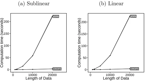
Further Simulations: Change in mean

In the main manuscript we looked at a change in mean model with a fixed number of changepoints and compared pDPA to CROPS with FPOP. Here we look at the results when the number of changepoints increases sublinearly and linearly with the number of data points.

(a) Sublinear

● ● ● ● ● ● ●

● ●

●

CROPS pDPA

0 50 100 150 200

(b) Linear

● ● ● ● ● ● ●

● ●

●

CROPS pDPA

0 50 100 150 200

[image:27.612.163.449.173.333.2]

(28)

Further Simulations: Change in mean and variance for normal model

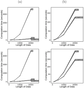
Similarly we revisit the model with a change in mean and variance to compare Segment Neighbourhood with CROPS with PELT and PELT with the recycled calculations for data sets with a sublinear and linear number of changepoints in respect to data length. Figure 2 shows the CPU cost for the 3 methods. We can then use this data and CROPS with PELT to explore penalty choice when we have a different number of changes. These results can be seen in Figure 3.

(a) ● ● ● ● ● ● ● ● ● ● ● ● ● ● ● PELT_speed PELT SN 0 1000 2000 3000

(b) ● ● ● ● ● ● ● ● ● ●_{PELT_speed} PELT 0 50 100 150

● ● ● ● ● ● ● ● ● ● ● ● ● ● ● PELT_speed PELT SN 0 1000 2000 3000

●● ● ● ● ● ● ● ● ●_{PELT_speed} PELT 0 50 100 150 200

[image:28.612.157.446.206.506.2]

(29)

● ● ● ● ● ● ● ● ● ● AIC HQ SIC 0 40 80 120 160

0 5000 10000 15000 20000 Length of Data

P enalty V alue ● ● ● ● ● ● ● ● ● ● ● ● ● ● ● ● ● ● ● ● ● ● ● ● ● ● ● ● ● ● ● ● ● ● ● ● ● ● ● ● ● ● ● ● ● ● ● ● ● ● ● ● ● ● ● ● ● ● ● ● ● ● ● ● ● ● ● ● ● ● ● ● ● ● ● ● ● ● ● ● SIC mean SIC sd HQ mean HQ sd 0.00 0.25 0.50 0.75 1.00

5000 10000 15000 20000 Length of Data

MSE ● ● ● AIC HQ SIC 0.80 0.85 0.90 0.95 1.00

Propor

tion of T

rue P ositiv es ● ● ● ● ● ● ● ● ● ● AIC HQ SIC 10 20 30 40 50

0 5000 10000 15000 20000 Length of Data

P enalty V alue ● ● ● ● ● ● ● ● ● ● ● ● ● ● ● ● ● ● ● ● ● ● ● ● ● ● ● ● ● ● ● ● ● ● ● ● ● ● ● ● ● ● ● ● ● ● ● ● ● ● ● ● ● ● ● ● ● ● ● ● ● ● ● ● ● ● ● ● ● ● ● ● ● ● ● ● ● ● ● ● SIC mean SIC sd HQ mean HQ sd 0.00 0.25 0.50 0.75 1.00

5000 10000 15000 20000 Length of Data

MSE ● ● ● AIC HQ SIC 0.80 0.85 0.90 0.95 1.00

Propor

tion of T

rue P

ositiv

[image:29.612.89.527.197.482.2]

es

(30)

Further Simulations: Change in mean and variance for the mis-specified model

We can also look at the situation where we have a mis-specified model with a sublinear and linear number of changes. The range of optimal penalty values and true and false positives found using different common penalty terms are shown in Figure 4

● ● ● ● ● ● ● ● ● ● AIC HQSIC 0 100 200 300 400

0 5000 10000 15000 20000

Length of Data

P enalty V alue ● ● ● AIC HQ SIC 0.00 0.25 0.50 0.75 1.00

0.00 0.25 0.50 0.75 1.00

Proportion of False Positives

Propor

tion of T

rue P ositiv es ● ● ● ● ● ● ● ● ● ● AIC HQ SIC 20 40 60

0 5000 10000 15000 20000

Length of Data

P enalty V alue ● ● ● AIC HQ SIC 0.00 0.25 0.50 0.75 1.00

0.00 0.25 0.50 0.75 1.00

Proportion of False Positives

Propor

tion of T

rue P

ositiv

[image:30.612.92.520.179.598.2]

es

(31)

Further regions where we have discrepancies in the Hi-C example

In the real data section of the main manuscript we showed regions of the chromosome where was have detected different segmentations with the different penalty terms. Below are a further 3 regions.

(a)

20 40 60 80 100

20

40

60

80

100

0 50 100 150 200 250

(b)

760 780 800 820 840

760

780