Coronal loop density profile estimated by forward modelling of EUV intensity

warwick.ac.uk/lib-publications

Original citation:

Pascoe, D. J. (David J.), Goddard, C. R., Anfinogentov, S. and Nakariakov, V. M. (Valery M.).

(2017) Coronal loop density profile estimated by forward modelling of EUV intensity.

Astronomy & Astrophysics, 600. L7.

Permanent WRAP URL:

http://wrap.warwick.ac.uk/86936

Copyright and reuse:

The Warwick Research Archive Portal (WRAP) makes this work by researchers of the

University of Warwick available open access under the following conditions. Copyright ©

and all moral rights to the version of the paper presented here belong to the individual

author(s) and/or other copyright owners. To the extent reasonable and practicable the

material made available in WRAP has been checked for eligibility before being made

available.

Copies of full items can be used for personal research or study, educational, or not-for-profit

purposes without prior permission or charge. Provided that the authors, title and full

bibliographic details are credited, a hyperlink and/or URL is given for the original metadata

page and the content is not changed in any way.

Publisher’s statement:

“Reproduced with permission from Astronomy & Astrophysics, © ESO”.

A note on versions:

The version presented here may differ from the published version or, version of record, if

you wish to cite this item you are advised to consult the publisher’s version. Please see the

‘permanent WRAP URL’ above for details on accessing the published version and note that

access may require a subscription.

March 5, 2017

Coronal loop density profile estimated by

forward modelling of EUV intensity

D. J. Pascoe, C. R. Goddard, S. Anfinogentov, and V. M. Nakariakov

Centre for Fusion, Space and Astrophysics, Department of Physics, University of Warwick, CV4 7AL, UK

e-mail:[email protected]

Received ¡date¿/Accepted ¡date¿

ABSTRACT

Aims.The transverse density structuring of coronal loops was recently calculated for the first time using the general damping profile for kink oscillations. This seismological method assumes a density profile with a linear transition region.We consider to what extent this density profile accounts for the observed intensity profile of the loop, and how the transverse intensity profile may be used to complement the seismological technique.

Methods.We use isothermal and optically transparent approximations for which the intensity of extreme ultraviolet (EUV) emission is proportional to the square of the plasma density integrated along the line of sight. We consider four different models for the transverse density profile; the generalised Epstein profile, the step function, the linear transition region profile, and a Gaussian profile. The effect of the point spread function is included and Bayesian analysis is used for comparison of the models.

Results.The two profiles with finite transitions are found to be preferable to the step function profile, which supports the interpretation of kink mode damping as being due to mode coupling. The estimate of the transition layer width using forward modelling is consistent with the seismological estimate.

Conclusions.For wide loops, i.e. those observed with sufficiently high spatial resolution, this method can provide an independent estimate of density profile parameters for comparison with seismological estimates. In the ill-posed case of only one of the Gaussian or exponential damping regimes being observed, it may provide additional information to allow a seismological inversion to be performed. Alternatively, it may be used to obtain structuring information for loops that do not oscillate.

Key words.Magnetohydrodynamics (MHD) – Sun: atmosphere – Sun: corona – Sun: magnetic fields – Sun: oscillations – Waves

1. Introduction

Large amplitude standing kink oscillations of coronal loops were first observed using the Transition Region And Coronal Explorer (TRACE; Aschwanden et al. 1999, 2002; Nakariakov et al. 1999). The Atmospheric Imaging Assembly (AIA;Lemen et al.

2012; Boerner et al. 2012) onboard the Solar Dynamics

Observatory (SDO) has greatly increased their detection (e.g.,

Zimovets & Nakariakov 2015;Goddard et al. 2016) and also led

to the discovery of the low amplitude decayless regime of stand-ing kink oscillations (Nistic`o et al. 2013; Anfinogentov et al. 2013, 2015). The strong damping of propagating kink waves and large amplitude standing kink waves is attributed to mode coupling or resonant absorption (e.g., reviews byPascoe 2014;

De Moortel et al. 2016), which we can also expect to

ap-ply to low amplitude decayless oscillations if the damping is compensated by some persistent driving mechanism (e.g.,

Nakariakov et al. 2016). The presence of a smooth transition

from the interior of an overdense coronal loop to the surround-ing environment provides a continuous range of local Alfv´en speeds. This condition allows mode couping to occur, which re-sults in the damping of kink oscillations as energy is tranfered to Alfv´en waves in the transition layer. The damping envelope of the kink oscillation is a continuous function (Hood et al. 2013) but may be approximated by a piecewise general damping profile

(Pascoe et al. 2013;Arregui et al. 2013) consisting of a Gaussian

stage (Pascoe et al. 2012, 2015) followed by an exponential stage (e.g., Ruderman & Roberts 2002; Goossens et al. 2002). Direct observational evidence for the Gaussian damping regime

(De Moortel et al. 2002;Pascoe et al. 2016c), the seismological

application of the general damping profile (Pascoe et al. 2016b,

2017), and the damping rates of spatially-resolved longitudi-nal harmonics (Pascoe et al. 2016a) support the interpretation of standing kink oscillations being damped by mode coupling.

The relationship between the density profile of a coronal loop and its appearance in EUV images such as those pro-duced by SDO/AIA is complicated and has motivated numerous studies (e.g.,De Moortel & Bradshaw 2008;Owen et al. 2009;

Taroyan & Bradshaw 2014; Yuan & Van Doorsselaere 2016).

The emission by plasma at a particular EUV wavelength de-pends on the density and temperature and may include con-tributions from a large number spectral lines. Coronal plasma is optically thin and so multiple structures or waves along the observational line of sight (LOS) appear superposed (e.g.,

De Moortel & Pascoe 2012). This may also include an

oscil-lating loop having a time-dependent superposition with itself

(Cooper et al. 2003a). The measured intensity also depends on

the properties of the particular instrument (e.g., Poduval et al. 2013). In this letter we consider a simple forward modelling pro-cedure that allows us to estimate the loop density profile. Our approach, described in Sect. 2, is similar to Aschwanden et al.

D. J. Pascoe et al.: Coronal loop density profile

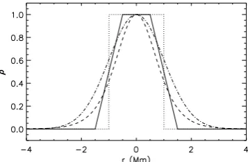
Fig. 1. Transverse loop density profiles used in our analysis; linear transition layer (Model L, solid line), Epstein profile (ModelE, dashed line), step function (ModelS, dotted line) and Gaussian (ModelG, dash-dot line).

1999;Aschwanden et al. 2000;Brooks et al. 2012;Antolin et al.

2015).

2. Method

We consider four different models for the transverse loop den-sity profile. The step function profile (Model S) describes an overdense loop in terms of an internal density ρ0, which is

greater than the external density ρe, and a minor radius R.

Analytical solutions for the behaviour of magnetohydrodynamic waves in a cylindrical loop with this profile have been derived

by Edwin & Roberts (1983). We consider the transverse

den-sity profileρprqfor a loop with a cylindrically symmetric cross-section and radial coordinaterto be

ρprq “ "

A, |r| ďR

0, |r| ąR, (1)

whereA“ρ0´ρeis the loop density enhancement.

The generalised symmetric Epstein profile (ModelE) is de-fined as

ρprq “Asech2

ˆ |r|

R ˙p

, (2)

which describes a smooth profile with a steepness determined by the parameter p. This profile has been used in many ana-lytical (e.g., Nakariakov & Roberts 1995; Cooper et al. 2003b;

Macnamara & Roberts 2011) and numerical studies (e.g.,

Nakariakov et al. 2005;Inglis et al. 2009;Pascoe & De Moortel

2014;Pascoe & Nakariakov 2016).

The linear transition layer profile (ModelL) is given by

ρprq “ $ ’ &

’ %

A, |r| ďr1 A

´

1´ r´r1 r2´r1

¯

, r1ă |r| ďr2

0, |r| ąr2

(3)

wherer1 “ Rp1´ϵ{2q,r2 “Rp1`ϵ{2q, andϵ “ l{Ris the

transition layer widthlnormalised toRand defined to be in the rangeϵ P r0,2s. The use of the linear transition layer profile in seismology is motivated by the availability of the full analytical solution for the damping envelope (Hood et al. 2013). However, the mechanism is insensitive to the details of fine structure (e.g.,

Terradas et al. 2008; Pascoe et al. 2011) and other profiles can

be considered, such as a sinusoidal (e.g.,Goossens et al. 2002;

Roberts 2008) or parabolic (Arregui et al. 2015) transition layer

profile.

We also consider a Gaussian density profile (ModelG; e.g.,

Aschwanden et al. 2007) given by

ρprq “Aexp

ˆ ´ r

2

2R2 ˙

. (4)

Examples of the four model profiles are given in Fig.1, with the magnitude of all parameters (A,R,p,ϵ) taken to be unity.

The step function density profile is a limiting case of both the generalised Epstein (pÑ 8) and linear transition layer (ϵÑ0) profiles. Since it describes the case with no continuous transition between the higher density core and lower density background, it is also the only profile for which the damping of kink oscillations cannot be accounted for by mode coupling. We use the Bayesian evidence for ModelS to be a common normalisation for our test of Models LandE (see Bayes factorKiS in Table1). We also

compare our models to Model G(using the Bayes factorKiG)

which describes a continuously varying density profile i.e. with no localisation of the transition layer.

Observations of hot coronal loops reveal them to be multi-thermal (e.g., Schmelz et al. 2010, 2014; Nistic`o et al. 2014). However,Aschwanden & Nightingale(2005) found the major-ity of cooler loops to be well-approximated as isothermal, and

Warren et al. (2008) found isolated loops typically have very

narrow temperature variation across the loop. DEM analysis of this particular loop suggests a temperature in the range 0.75– 1.25 MK (Pascoe et al. 2017). The use of the isothermal approx-imation allows the intensity profile to be calculated simply as the square of the density integrated along the LOS. For Model S, the integrated loop intensity could be readily calculated asA2_d,

where the loop depthdalong the LOS is the chord length of the circular loop cross-section. However, since equivalent expres-sions are not available for the other models we instead calculate the loop intensity numerically by constructing a 2D (Cartesian) density profile for the radial profiles given in Eqs. (1) – (4) with

r“ b

px´x0q 2

` py´y0q 2_.

Herexis the direction transverse to the loop, the loop centre is atx0, andyis the direction along the LOS. The values ofyand

y0 are arbitrary and so we take yto have the same range as x

and y0 “ xyy. In addition to the contribution from the dense

loop given by Eqs. (1)–(4), the density profile also contains a background contribution which is described by a second or-der polynomial in space. This corresponds to the emission from the background plasma (including any structures other than the loop). The intensity profile is smoothed to simulate the effect of the point spread function (PSF). We use a Gaussian kernel with

σ“1.019 pixels, corresponding to the 171Å SDO/AIA channel

(Grigis et al. 2013). The measured intensity profile consists of 44

data points while our 2D density profile is calculated at a higher resolution of 440ˆ440 pixels i.e. a multiplication factor of 10 (convergence tests indicate consistent results for factors ě 7). The model intensity profile is then interpolated onto the original transverse coordinates and compared with the observational data

Dusing the Bayesian inference and Markov Chain Monte Carlo (MCMC) methods described inPascoe et al.(2017). Calculating the Bayes factorBi j(Jeffreys 1961;Kass & Raftery 1995) allows

quantitative comparison of our four density profile models

Bi j“

PpD|Miq PpD|Mjq

, Ki j“2 lnBi j. (5)

Values ofKi jgreater than 2, 6 and 10 correspond to “positive”,

“strong”, and “very strong” evidence for model MioverMj,

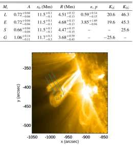
Table 1.Parameters for our density profile modelsMifor slit 10.

Mi A x0(Mm) R(Mm) ϵ,p KiS KiG

L 0.72`<sub>´</sub>0<sub>0</sub>.<sub>.</sub>04<sub>04</sub> 11.5`_´0₀._.1₁ 4.51`<sub>´0</sub>0.<sub>.</sub>12<sub>13</sub> 0.59<sub>´</sub>`₀0._.14₁₅ 20.6 46.3

E 0.72`<sub>´</sub>0<sub>0</sub>.<sub>.</sub>04<sub>04</sub> 11.5`_´0₀._.1₁ 4.68`<sub>´0</sub>0.<sub>.</sub>13<sub>13</sub> 3.85<sub>´</sub>`₀1._.69₉₄ 19.6 45.3

S 0.66`<sub>´</sub>0<sub>0</sub>.<sub>.</sub>04<sub>04</sub> 11.5<sub>´</sub>`0_0..1₁ 4.47_´`₀0._.15₁₅ – – 25.6

G 1.06`<sub>´</sub>0<sub>0</sub>.<sub>.</sub>14<sub>11</sub> 11.7<sub>´</sub>`₀0_..3₃ 3.68`_´0_0..59₄₅ – ´25.6 –

-1050 -1000 -950 -900 -850

x (arcsec) -500

-450 -400 -350

y (arcsec)

-1050 -1000 -950 -900 -850

-500 -450 -400 -350

1 6 12

Fig. 2.SDO/AIA 171 Å image of the analysed loop, observed 08:58:00 UT on 30 May 2012. The blue lines indicate the loca-tions of the 12 slits used to generate transverse intensity profiles.

3. Results

We apply the method described in Sect. 2 to Loop #3 from

Pascoe et al.(2016b,2017), chosen since it has the largest radius

(R«4 Mm) of the four coronal loops analysed and so provides the greatest spatial information. Our method did not produce well-constrained values ofϵfor the three other loops, which have

R ≲2 Mm, although instruments with higher spatial resolution than SDO/AIA would allow us to extend its applicability. This is also the loop for which the seismological estimate forϵis most narrowly constrained by its oscillation. The seismologically de-termined density profile parameters calculated in Pascoe et al.

(2017) areρ0{ρe “2.96_´0`1.<sub>.</sub>00<sub>66</sub> andϵ “0.49`0_´0._.23₁₂, where the

pa-rameter ranges correspond to the 95% credible intervals. The lower (higher) estimate for the density contrast (layer width) in comparison with those inPascoe et al.(2016b) results from tak-ing the decayless component into account when analystak-ing the kink oscillation. The loop is shown in Fig.2with the locations of 12 equally spaced slits used to generate transverse intensity profiles indicated by blue lines. The minor radiusRof the loop is observed to increase with heightz(measured along the loop axis). Consequently, slits taken higher up provide greater spatial information for the loop than those lower down. Higher slits may also benefit from fewer additional EUV sources along the LOS. On the other hand, we avoid slits too close to the apex of the loop (z„rc´R«70 Mm, wherercis the loop major radius) since

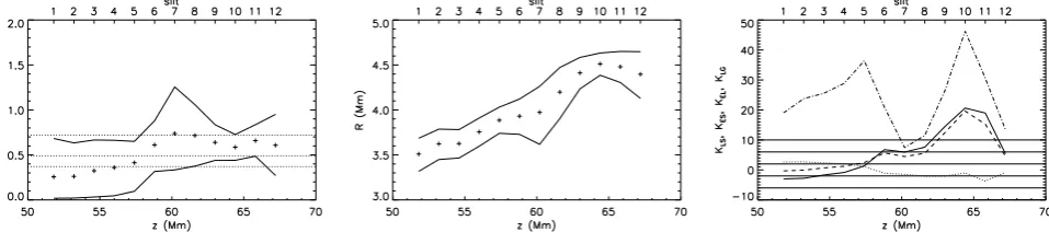
here the intensity profile is complicated by the curved geometry. Each intensity profile is analysed using the four models. Figure 3 and Table1 summarise the results for one particular slit (slit 10). The left panel of Fig.3 shows the observational intensity profile (symbols) and the profile for Model L (blue

line). The middle panel shows the histogram forϵ. The dotted and dashed lines denote the median value and the 95% credible interval, which also correspond to the values quoted in Table1. The right panel shows the loop density profiles (using median values of sampled parameters) for each of the four models and indicates that modelsEandLproduce very similar results.

Figure4shows the dependence ofϵ andRwith height for ModelL. The loop is found to expand with height, whileϵ re-mains consistent with the seismological estimate (dotted lines). Generally, the value of ϵ obtained using forward modelling is less constrained than the seismological estimate. The right panel shows Bayes factors calculated for model comparison. For lower slits (with smaller R) there is no statistical evidence to prefer Model Lor Eover ModelS, indicating the effects of LOS in-tegration over a circular cross-section and the PSF are suffi -cient to account for the smoothness of the loop intensity profile. However, the evidence in favour of the two profiles with transi-tion layers greatly increases over the step functransi-tion for higher slits with effectively higher resolution, surpassing the requirements for “strong” (Ki j ą 6) and “very strong” (Ki j ą10) evidence.

For this data, there is no statistical evidence to distinguish be-tween ModelsLandE(|KEL|≲2), consistent with these models

producing very similar results. ModelsL,E, andS all have very strong evidence over ModelG. For this loop we therefore find that a density model with a transition region (Lor E) provides a better account of the intensity profile than a profile without a transition region (S). On the other hand, the transition region is sufficiently localised that there is greater statistical evidence for ModelS than the fully inhomogeneous case of ModelG.

4. Discussion

This study presents statistical evidence for the existence of a lo-calised transition layer in the density profile of the coronal loop considered. Furthermore, the size of this layer is consistent for ModelsLandE(Fig.3), and with the independent seismological estimate using a damped kink oscillation (Fig.4).

For observations of kink oscillations for which only the Gaussian or exponential damping regime are observed, in the in-version problem is ill-posed since the damping timeτis a func-tion of the density contrast and the layer width. Due to the effect of LOS integration, forward modelling of EUV intensity cannot reveal the density contrast of coronal loops since the intensity contrast is also function of an unknown column depth. However, we have demonstrated that the structure parameterϵmay be es-timated by forward modelling of the transverse intensity pro-file, and so combining this with the measuredτcould allow the density contrast to be inferred. It may also be used to obtain structuring information for loops that do not oscillate, or to re-veal any time-dependent variations in the cross-sectional profile

(Aschwanden & Schrijver 2011) which may be associated with

non-linear effects (Goddard & Nakariakov 2016).

Acknowledgements. This work is supported by the European Research Council under theSeismoSunResearch Project No. 321141 (DJP, CRG, SA, VMN) and the STFC consolidated grant ST/L000733/1 (VMN). The data is used courtesy of the SDO/AIA team.

References

Anfinogentov, S., Nistic`o, G., & Nakariakov, V. M. 2013, A&A, 560, A107 Anfinogentov, S. A., Nakariakov, V. M., & Nistic`o, G. 2015, A&A, 583, A136 Antolin, P., Vissers, G., Pereira, T. M. D., Rouppe van der Voort, L., & Scullion,

E. 2015, ApJ, 806, 81

D. J. Pascoe et al.: Coronal loop density profile

Fig. 3.Left171 Å EUV intensity (symbols) across the loop is described by ModelL(blue line) which includes a background trend described by a second order polynomial. The shaded regions represent the 99% confidence intervals for the intensity predicted by the model, with (red) and without (blue) modelled noise. The vertical dotted and dashed lines denotex0andx0˘R, respectively.Middle

Histogram of normalised layer widthϵbased on 105_{samples. The vertical dotted and dashed lines denote the median value and the}

95% credible interval, respectively.RightLoop density profiles for ModelsL(solid),E(dashed),S (dotted), andG(dash-dot).

Fig. 4.Normalised layer width ϵ (left) and loop radiusR (middle) estimated by forward modelling. The symbols show the me-dian values while the solid curves denote the 95% credible interval. The horizontal dotted lines correspond to the seismologically estimated values. Therightpanel shows the Bayes factorsKLS (solid),KES (dashed),KEL(dotted), andKLG(dash-dot).

Arregui, I., Soler, R., & Asensio Ramos, A. 2015, ApJ, 811, 104

Aschwanden, M. J., de Pontieu, B., Schrijver, C. J., & Title, A. M. 2002, Sol. Phys., 206, 99

Aschwanden, M. J., Fletcher, L., Schrijver, C. J., & Alexander, D. 1999, ApJ, 520, 880

Aschwanden, M. J. & Nightingale, R. W. 2005, ApJ, 633, 499

Aschwanden, M. J., Nightingale, R. W., & Alexander, D. 2000, ApJ, 541, 1059 Aschwanden, M. J., Nightingale, R. W., Andries, J., Goossens, M., & Van

Doorsselaere, T. 2003, ApJ, 598, 1375

Aschwanden, M. J., Nightingale, R. W., & Boerner, P. 2007, ApJ, 656, 577 Aschwanden, M. J. & Schrijver, C. J. 2011, ApJ, 736, 102

Boerner, P., Edwards, C., Lemen, J., et al. 2012, Sol. Phys., 275, 41 Brooks, D. H., Warren, H. P., & Ugarte-Urra, I. 2012, ApJ, 755, L33 Cooper, F. C., Nakariakov, V. M., & Tsiklauri, D. 2003a, A&A, 397, 765 Cooper, F. C., Nakariakov, V. M., & Williams, D. R. 2003b, A&A, 409, 325 De Moortel, I. & Bradshaw, S. J. 2008, Sol. Phys., 252, 101

De Moortel, I., Hood, A. W., & Ireland, J. 2002, A&A, 381, 311 De Moortel, I. & Pascoe, D. J. 2012, ApJ, 746, 31

De Moortel, I., Pascoe, D. J., Wright, A. N., & Hood, A. W. 2016, Plasma Physics and Controlled Fusion, 58, 014001

Edwin, P. M. & Roberts, B. 1983, Sol. Phys., 88, 179 Goddard, C. R. & Nakariakov, V. M. 2016, A&A, 590, L5

Goddard, C. R., Nistic`o, G., Nakariakov, V. M., & Zimovets, I. V. 2016, A&A, 585, A137

Goossens, M., Andries, J., & Aschwanden, M. J. 2002, A&A, 394, L39 Grigis, P., Yingna, S., & Weber, M. 2013, Tech. Rep., AIA team Hood, A. W., Ruderman, M., Pascoe, D. J., et al. 2013, A&A, 551, A39 Inglis, A. R., van Doorsselaere, T., Brady, C. S., & Nakariakov, V. M. 2009,

A&A, 503, 569

Jeffreys, H. 1961, Theory of Probability, 3rd edn. (Oxford)

Kass, R. E. & Raftery, A. E. 1995, Journal of the American Statistical Association, 90, 773

Lemen, J. R., Title, A. M., Akin, D. J., et al. 2012, Sol. Phys., 275, 17 Lenz, D. D., Deluca, E. E., Golub, L., et al. 1999, Sol. Phys., 190, 131 Macnamara, C. K. & Roberts, B. 2011, A&A, 526, A75

Nakariakov, V. M., Anfinogentov, S. A., Nistic`o, G., & Lee, D.-H. 2016, A&A, 591, L5

Nakariakov, V. M., Ofman, L., Deluca, E. E., Roberts, B., & Davila, J. M. 1999, Science, 285, 862

Nakariakov, V. M., Pascoe, D. J., & Arber, T. D. 2005, Space Sci. Rev., 121, 115 Nakariakov, V. M. & Roberts, B. 1995, Sol. Phys., 159, 399

Nistic`o, G., Anfinogentov, S., & Nakariakov, V. M. 2014, A&A, 570, A84 Nistic`o, G., Nakariakov, V. M., & Verwichte, E. 2013, A&A, 552, A57 Owen, N. R., De Moortel, I., & Hood, A. W. 2009, A&A, 494, 339 Pascoe, D. J. 2014, Research in Astronomy and Astrophysics, 14, 805 Pascoe, D. J., Anfinogentov, S., Nistic`o, G., Goddard, C. R., & Nakariakov,

V. M. 2017, A&A

Pascoe, D. J. & De Moortel, I. 2014, ApJ, 784, 101

Pascoe, D. J., Goddard, C. R., & Nakariakov, V. M. 2016a, A&A, 593, A53 Pascoe, D. J., Goddard, C. R., Nistic`o, G., Anfinogentov, S., & Nakariakov,

V. M. 2016b, A&A, 589, A136

Pascoe, D. J., Goddard, C. R., Nistic`o, G., Anfinogentov, S., & Nakariakov, V. M. 2016c, A&A, 585, L6

Pascoe, D. J., Hood, A. W., de Moortel, I., & Wright, A. N. 2012, A&A, 539, A37

Pascoe, D. J., Hood, A. W., De Moortel, I., & Wright, A. N. 2013, A&A, 551, A40

Pascoe, D. J. & Nakariakov, V. M. 2016, A&A, 593, A52 Pascoe, D. J., Wright, A. N., & De Moortel, I. 2011, ApJ, 731, 73

Pascoe, D. J., Wright, A. N., De Moortel, I., & Hood, A. W. 2015, A&A, 578, A99

Poduval, B., DeForest, C. E., Schmelz, J. T., & Pathak, S. 2013, ApJ, 765, 144 Roberts, B. 2008, in IAU Symposium, Vol. 247, IAU Symposium, ed. R. Erd´elyi

& C. A. Mendoza-Briceno, 3–19

Ruderman, M. S. & Roberts, B. 2002, ApJ, 577, 475

Schmelz, J. T., Pathak, S., Brooks, D. H., Christian, G. M., & Dhaliwal, R. S. 2014, ApJ, 795, 171

Schmelz, J. T., Saar, S. H., Nasraoui, K., et al. 2010, ApJ, 723, 1180 Taroyan, Y. & Bradshaw, S. J. 2014, Sol. Phys., 289, 1959 Terradas, J., Arregui, I., Oliver, R., et al. 2008, ApJ, 679, 1611

Warren, H. P., Ugarte-Urra, I., Doschek, G. A., Brooks, D. H., & Williams, D. R. 2008, ApJ, 686, L131