Low Density Cluster Separators for Large, High Dimensional, Mixed and Non Linearly Separable Data

(1)

Low-Density Cluster Separators for Large,

High-Dimensional, Mixed and

Non-Linearly Separable Data.

Submitted by

Katie R Yates B.Sc.(Hons.), M.Res to

Lancaster University for the degree of Doctor of Philosophy

in the subject of

(2)

Low-Density Cluster Separators for Large, High-Dimensional,

Mixed and Non-Linearly Separable Data.

Katie R Yates Bsc. (Hons), MRes.

Submitted for the degree of Doctor of Philosophy at Lancaster University.

October 2017

Abstract

The location of groups of similar observations (clusters) in data is a well-studied problem, and has many practical applications. There are a wide range of approaches to clustering, which rely on different definitions of similarity, and are appropriate for datasets with dif-ferent characteristics. Despite a rich literature, there exist a number of open problems in clustering, and limitations to existing algorithms.

This thesis develops methodology for clustering high-dimensional, mixed datasets with complex clustering structures, using low-density cluster separators that bi-partition datasets using cluster boundaries that pass through regions of minimal density, separating regions of high probability density, associated with clusters. The bi-partitions arising from a succession of minimum density cluster separators are combined using divisive hierarchical and parti-tional algorithms, to locate a complete clustering, while estimating the number of clusters.

(3)

space, in which a linear separator permits the correct identification of non-linearly separable clusters in the original dataset.

(4)

To David for all your love and support throughout my PhD. and every other aspect of my life for the past 10 years.

To Mum and Dad. You have always been there for me in every way possible, and I could not have achieved a fraction of what I have without your never ending love, guidance and encouragement.

To Karen for being the best sister and role model. Your achievements have always encouraged me to follow in your footsteps.

To Nanna for always encouraging me to learn. For as long as I can remember, you were always there to ask me questions and teach me new things.

(5)

Acknowledgements

I would like to thank my supervisors Nicos Pavlidis and Chris Sherlock. This project was started under difficult circumstances, and without your support I would not have made it past the first year of my PhD. Nicos, your enthusiasm and words of wisdom have got me through the last three years and I have learnt more from you than you would ever take credit for. From helping me with my writing to debugging my code with me, I could not have asked for a more dedicated supervisor. I would also like to thank Sotiris Tasoulis for his con-tributions to Chapter 6 of this thesis.

I would also like to thank all the staff and students at the STOR-i centre for doctoral training. Having you there through difficult times to talk about the stresses of PhD. life over a cup of tea or lunch has made this whole experience much less intimidating. I would especially like to thank David Hofmeyer, for your academic contributions to Chapter 4 of this thesis, and also for your words of advice through the first two years of my PhD.

Thank you to my very dear friends Helen and Lucy for always being there with a smile to make even the worst days in the office better. From singing along to our music in the car to our Euro-vision parities, I could not have asked for better friends to go through my time at Lancaster with.

(6)

Declaration

I declare that the work in this thesis has been done by myself and has not been submitted elsewhere for the award of any other degree.

All the work produced in this thesis was done so in collaboration with my supervisor Nicos Pavlidis. The work in Chapter 4 and Chapter 6 also involved collaboration with David Hofmeyr and Sotiris Tasoulis respectively.

Preliminary work from Chapter 5 is published as Yates, K. R. and Pavlidis, N. G. (2016). Minimum density hyperplanes in the feature space.In Big Data (Big Data), 2016 IEEE International Conference on, pages 3613–3618. IEEE.

The work included in all three main chapters of this thesis is in preparation for submission as journal papers.

Katie R Yates

(7)

8 Conclusion 195 8.1 Summary of Contributions . . . 195 8.2 Further Work . . . 198 8.2.1 Tuning the Kernel . . . 198 8.2.2 Multi-Objective Optimisation for Random Projection Selection . . 200 8.2.3 Alternative Splitting Rule for Random Projections . . . 201 8.2.4 Higher-Dimensional Subspaces for Random Projection . . . 202

(10)

List of Figures

3.1 Example structure in continuous representation of simulated mixed data gen-erated by MixGen1. . . 56 3.2 Example structure in continuous representation of simulated mixed data

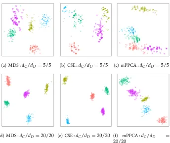
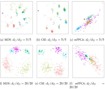
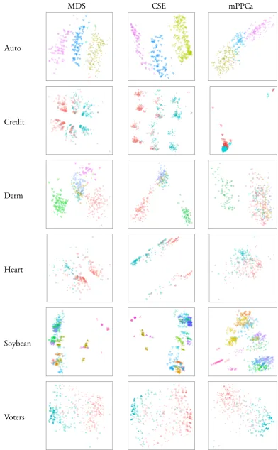
gen-erated by MixGen2. . . 57 3.3 Two-dimensional continuous representations of real datasets from MDS, CSE

and mPPCA. . . 62 3.4 Boxplot of regret based on NMI for continuous representations produced by

MDS, CSE and mPPCA. . . 65 4.1 Illustration of local minimaIˆ(v,b)and the resulting hyperplane separators from

constrained optimisation with 50 random initialisations for the S4 dataset. . 73 4.2 Separating hyperplaneH(v,b), estimated density of the projections ofX onto

v(black line),Iˆ(v,·), and penalised objective function, f(v,·), forη =0.01

andε={0.1, 0.3, 0.9}(burgundy,orange and green lines respectively). . . 74 4.3 Illustration of the resulting hyperplane separators from the projection pursuit

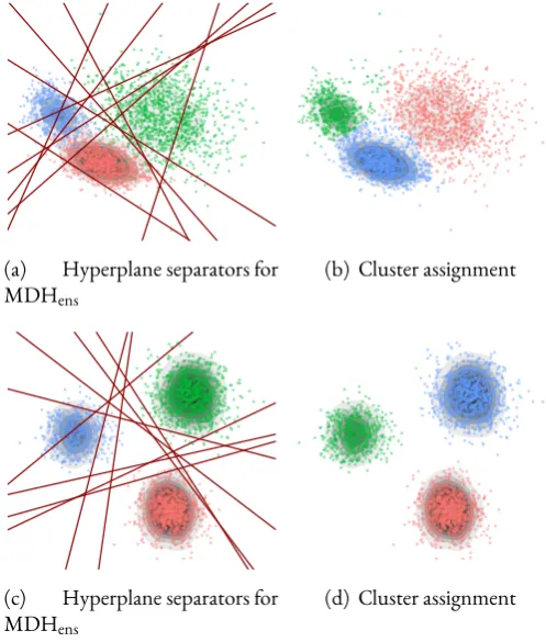
formulation with 50 random initialisations for the S4 dataset. . . 75 4.4 Clusters identified by divisive algorithm MDHhier. . . 80 4.5 Clusters identified by partitional algorithm MDHens. . . 80 4.6 Example structure in continuous simulated data produced by projecting onto

the first two principal components . . . 88 4.7 Example structure in continuous representation of simulated mixed data

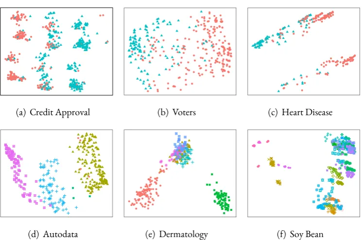
pro-duced using CSE . . . 89 4.8 Box plot of regret based on the NMI over continuous real datasets . . . 94 4.9 Two-dimensional visualisation of mixed real datasets after the application of

CSE . . . 95 4.10 Box plot of regret with respect to NMI over mixed real datasets . . . 97 4.11 Image segmentation from MDHhier, MDHensand competing algorithms . . 99 5.1 Boxplots of regret for each algorithm considered based on NMI over

bench-mark datasets. Mean regret is depicted with a red dot. . . 121 6.1 Increase in success ratio with increasing number of random projections for

sim-ulated datasets with 30 clusters in 1,000, 10,000 and 19,000 dimensions and real benchmark datasets summarised in Section 6.3.4. . . 149 6.2 CPU time for a binary split with increasing numbers of observations and

di-mensionality for RP, PCA, ICA and MDH. . . 151 6.3 CPU time for a full clustering hierarchy with increasing numbers of clusters and

dimensionality for RP, PCA, ICA and MDH. . . 152 6.4 Four dimensions of a simulated dataset. . . 154 6.5 PCA projections of example simulated datasets with 10 clusters as

(11)

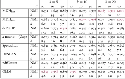
6.6 Boxplots of clustering performance from hierarchies of low-density separators located by RP approaches, PCA, ICA and MDH as well ask-means++ over 30 replications for simulated datasets with 10 and 50 clusters, 1,000 and 19,000 di-mensions. . . 155 6.7 Boxplots of estimated number of clusters from hierarchies of low-density

sep-arators located by RP approaches, PCA, ICA and MDH as well ask-means++ over 30 replications for simulated datasets with 10 and 50 clusters, 1,000 and 19,000 dimensions. . . 157 6.8 Boxplots of clustering performance from hierarchies of low-density separators

located by RP approaches, PCA, ICA and MDH as well ask-means++ over real datasets. . . 160 6.9 Boxplots of estimated number of clusters from hierarchies of low-density

sep-arators located by RP approaches, PCA, ICA and MDH as well ask-means++ over real datasets. . . 163 6.10 Boxplots of regret with respect to NMI for the four optimality criteria for RP

approaches. . . 165 6.11 Increase in success ratio with increasing number of random projections for mapped

feature vectors of real benchmark datasets summarised in Table 6.1. . . 167 6.12 Boxplots of clustering performance from hierarchies of low-density separators

located by RP approaches with 100 projections, PCA, ICA and MDH as well ask-means++ over mapped feature vectors of real datasets. . . 170 6.13 Boxplots of clustering performance from hierarchies of low-density separators

located by RP approaches with 1,000 projections, PCA, ICA and MDH as well ask-means++ over mapped feature vectors of real datasets. . . 171 6.14 Boxplots of estimated number of clusters from hierarchies of low-density

sep-arators located by RP approaches with 100 projections, PCA, ICA and MDH as well ask-means++ over mapped feature vectors of real datasets. . . 174 6.15 Boxplots of estimated number of clusters from hierarchies of low-density

sep-arators located by RP approaches with 1,000 projections, PCA, ICA and MDH as well ask-means++ over mapped feature vectors of real datasets. . . 175 6.16 Boxplots of regret with respect to NMI for the four optimality criteria for RP

approaches using 100 projections over mapped feature vectors of real datasets. 177 6.17 Boxplots of regret with respect to NMI for the four optimality criteria for RP

approaches using 1,000 projections over mapped feature vectors of real datasets. 178 7.1 Increase in success ratio for a bi-partition of univariate random projections of

the feature vectors using 2-means and spectral clustering with increasing num-ber of random projections for real benchmark datasets summarised in Table 6.1. 190 7.2 Boxplots of clustering performance of RP approaches using 100 projections,

bisecting kernelk-means and hierarchical spectral clustering over mapped fea-ture vectors of real datasets. . . 192 7.3 Boxplots of clustering performance of RP approaches using 1,000 projections,

(12)

List of Tables

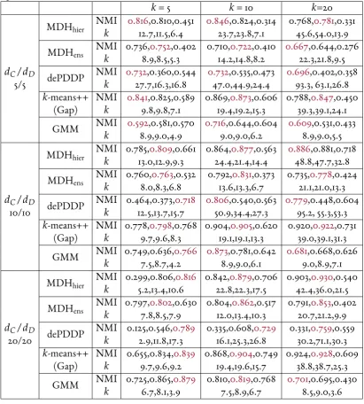
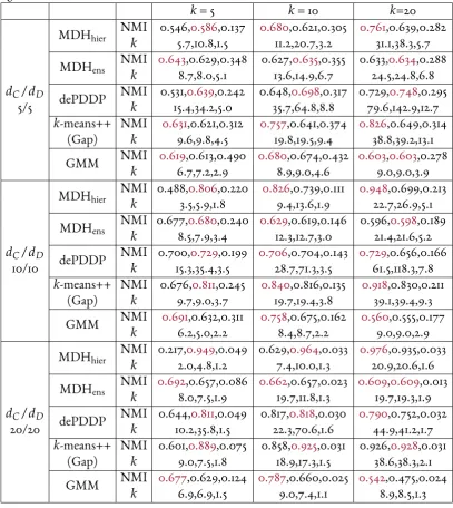
3.1 Mean clustering performance with respect to NMI and estimated number of clusters from MDS,CSE,mPPCA representations of data generated by MixGen1. The best continuous representation for each scenario and choice of clustering algorithm is highlighted in red. . . 58 3.2 Mean clustering performance with respect to NMI and estimated number of

clusters from MDS,CSE,mPPCA representations of data generated by MixGen2. The best continuous representation for each scenario and choice of clustering algorithm is highlighted in red. . . 59 3.3 Summary of mixed benchmark datasets. . . 61 3.4 Clustering performance with respect to NMI across real benchmark datasets.

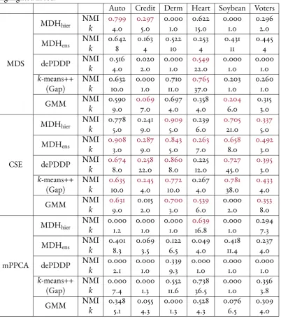
The representation which resulted in the best performance for each clustering algorithm is highlighted in red. . . 63 4.1 Clustering performance on simulated continuous datasets. The top row of each

cell of the table reports NMI and the second the estimated number of clusters. Each cell reports mean performance over 30 experiments. . . 90 4.2 Clustering performance on simulated mixed datasets. The top row of each cell

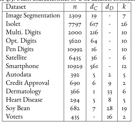
of the table reports NMI and the second the estimated number of clusters. Each cell reports mean performance over 30 experiments. . . 92 4.3 Main characteristics of UCI datasets considered. . . 92 4.4 Clustering performance on continuous real datasets. The top row of each cell

of the table reports NMI and the second the estimated number of clusters (when applicable). For the non-deterministic MDHhierthe mean performance over 30 runs is given. . . 93 4.5 Clustering performance on mixed real datasets. In each cell of the table the first

row reports NMI and the second the estimated number of clusters (when ap-plicable). For the non-deterministic MDHhierthe mean performance over 30 runs is given. . . 96 5.1 Main characteristics of real datasets considered. . . 118 5.2 Clustering performance of KMDHhier, S-KMDHhier, K-dePDDP, Kernelk

(13)

1

Introduction

The task of locating groups of related objects in data is a well studied problem in machine learning, statistics, data mining and pattern recognition. This has a number of practical ap-plications including:

• Business and marketing : In market research, it is useful to partition the population of customers into groups with similar buying habits to infer relationships between them, assess strategic opportunities and identify competitive threats (Hruschka,

1986). In marketing and advertising, recommender systems require groups of simi-lar products and customers allowing targeted marketing strategies where simisimi-lar items are recommended to similar customers (Hameed et al.,2012).

• Computer science : Image segmentation can be used to divide a digital image into smaller segments which can be used for object recognition and border detection (Zhang,1996). Web searching relies on grouping web pages with similar content to help locate the most relevant results as quickly as possible (Beeferman and Berger,

2000).

• Security : Learning groups of individuals with similar behaviour, for example spend-ing patterns, allows the detection of network intrusions and potentially malicious behaviour (Portnoy et al.,2001).

• Biology and medicine : Monitoring the level of expression of groups of genes over time allows the understanding of the roles of different genes (Zhao and Karypis,

2005). In medical imaging, identifying regions of different tissue types is used to identify different tumours and assess the effect of treatments (Masulli and Schenone,

1999).

• Physical sciences : In astrophysics, grouping objects allows the detection of regions of interest such as galaxies and gas clouds (Zentner et al.,2005).

(14)

observa-tions with associated class labels is used to construct the predictive model for the subsequent grouping of unlabelled observations (Theodoridis and Koutroumbas,2008). In many ap-plications, knowledge of the true class labels may be expensive or impossible to obtain. In the absence of such information, the problem becomes one ofunsupervised learningor clus-tering, which is considered in this thesis. Clustering requires a user specified definition of similarity, which will determine the groups orclusters. The objective of clustering is to parti-tion the set of observaparti-tionsX ={xi}n_i=1wherexi ∈Rdintokdisjoint subsets (clusters),

C ={C1, ...,Ck} (1.1)

such that

C_i∩C_j =∅ ∀ i,j ∈1, ...,k i ̸= j (1.2)

C₁∪...∪C_k =X (1.3)

so as to maximise similarity between observations within the same cluster, while minimis-ing similarity between observations in different clusters. There exist a variety of ways to define similarity, thus there is no universally adopted definition of what constitutes a cluster (Berkhin,2006). Different specifications of similarity give rise to numerous approaches to clustering, some of which are discussed in Chapter 2.

(15)

1.1 Thesis Aims and Structure

1.1.1 Aims

The aim of this thesis is to address the challenges of identifying clusters in datasets with large numbers of diverse features and complex clustering structures, while estimating their num-ber. The approaches proposed are methodological ideas, which may be applied in a variety of application areas, but are not designed for any specific clustering task. These approaches do not attempt to completely solve all of the problems discussed in Section 2.2, associated with clustering complex datasets, but offer potential techniques to allow cluster identifi-cation in datasets where current methodology is limited. With the exception of Chapter 7, the methodology presented in this thesis relies on locating low-density cluster boundaries, which separate clusters corresponding to regions of high probability density, as defined in the density-based approach to clustering. The relevant definitions which underpin the algo-rithms proposed in this thesis are presented in Section 2.3.

1.1.2 Structure and Contributions

The body of this thesis consists of five chapters. Chapter 3 investigates the production of continuous representations of mixed datasets. This evaluates the performance of a variety of clustering algorithms over three different continuous representations of simulated and real-world mixed datasets. The production of a suitable continuous representation then permits the application of any clustering algorithm that makes the assumption of continuous ob-servations, including the projective density-based clustering algorithms that are proposed in this thesis. To our knowledge, a comparative study into continuous representations of mixed data for clustering has not been undertaken in the literature.

(16)

which are able to identify arbitrary numbers of high-density clusters in high-dimensional datasets by combining hyperplane separators that intersect regions of minimal probabil-ity densprobabil-ity. These hyperplanes are located using the minimum densprobabil-ity hyperplane (MDH), proposed byPavlidis et al.(2016) for binary partitions, and are computed using one-dimensional projections of the data only, avoiding the problems associated with density estimation on high dimensions. The algorithms proposed extend the MDH approach to clustering by al-lowing the identification of multiple clusters, and estimating their number. Through an appropriate continuous representation of datasets with mixed attributes, we further extend the applicability of the proposed approaches to mixed datasets, upon which density-based clustering would ordinarily not be possible. The proposed algorithms extend the current literature by permitting the application of the density-based approach to clustering to large, high-dimensional and mixed datasets. Our algorithms locate very high-quality clustering results, often outperforming alternative well-established and sate-of-the-art clustering algo-rithms across a variety of datasets.

(17)

mapping exists).

The dimensionality of the optimisation problem to locate the MDH in the feature space is determined by the number of observations, and for large datasets the location of the MDH in the feature space is computationally expensive. Therefore, we consider reducing the search space using an appropriate subspace of the feature space, in which an approxi-mate minimum density separator of the feature vectors may be computed. We also include an equivalent approach to locate minimum density hyperplane separators of the feature vec-tors using their projections onto an orthonormal basis of the space spanned by them, that is more straightforward to implement than the formulation of the MDH using the kernel ma-trix. The bi-partitions of the feature vectors located by the MDH are combined in a divisive algorithm to allow the identification of multiple clusters that are not correctly identifiable by hyperplane separators in the data space, and automatically estimate their number.

(18)

in a divisive algorithm, that automatically estimates the number of clusters. The use of RP to locate approximate minimum density cluster boundaries in one-dimensional subspaces is a novel idea. This approach permits the application of minimum density cluster separation in large, high-dimensional datasets, where the optimisation techniques proposed in Chap-ters 4 and 5 are practically infeasible.

(19)

2

Literature Review

This chapter, provides a overview of common cluster definitions and associated algorithms. It is worth noting that some formulations of the clustering problem are NP-hard, making this a non-trivial problem. This is not an exhaustive review of the wide variety of the clus-tering literature, however, the relevant concepts for the remainder of the thesis are discussed. In addition, Section 2.2 presents the challenges in clustering, which this work aims to ad-dress. Finally, Section 2.3 presents the relevant definitions of the clusters and cluster separa-tors which are located by the algorithms proposed in this thesis.

2.1 Clustering

In this section, existing approaches to clustering are discussed. These are categorised by the cluster definition assumed in each case. In addition, clustering algorithms can be divided into two approaches,hierarchicalandﬂat(partitional). Hierarchical clustering locates a nested structure of partitions, defined as follows. Given two partitionsB = {B1, ...,Bk}

andC = {C₁, ...,Cm}as defined in Eqs. (1.1)-(1.3),Bis nested intoCif every component

ofB,Bi ⊂ Cjfor one of the components ofC. This hierarchy of nested partitions is

sum-marised in a cluster tree or dendrogram, showing the clustering structure evident at different levels of similarity (Johnson,1967). Meanwhile, partitional methods produce an overall clus-teringC ={C1, ...,Ck}as defined in Eqs. (1.1)-(1.3) on a single level. Hierarchical clustering

(20)

structure generally allows superior detection of clusters on different scales. The majority of the algorithms outlined in this section are partitional, and are discussed separately to some well established methods for hierarchical clustering. It is worth noting that there exist hi-erarchical adaptations of a number of the partitional approaches discussed, but these are omitted for brevity and will be included, where relevant, in later chapters.

Despite the multitude of similarity measures, it is natural to assume that information about similarity exists in the spatial proximity between the observations. The evaluation of this spatial proximity is a non-trivial problem, and there exist multiple distance metrics that may be applied in practice. A complete discussion of the wide variety of proximity mea-sures, which are appropriate for different data types and clustering applications is beyond the scope of this introduction, however, a comprehensive overview of these methods is pro-vided byGan et al.(2007).

For continuous data, the most common distance metrics are special cases of the Minkowski distance,

D_ij =

( d

∑

l=1

|x_i_,_l−x_j_,_l|r

)1/r

; r⩾1

wherex_i_,_lis thelth dimension of datumx_i ∈ X = {x_i}n_i₌₁, wherex_i ∈ Rd. Tak-ingr = 1, 2,∞, gives the Manhattan, Euclidean and maximum distance metrics respec-tively. The most widely used of these metrics is the Euclidean distance, hence this is assumed throughout this section.

2.1.1 Hierarchical Clustering

(21)

distinct approaches. The divisive approach begins with all observations in a single cluster and sequentially divides this into smaller groups. By contrast, the agglomerative approach begins with all observations belonging to individual clusters, and merges the most similar groups at each level of the hierarchy.

Agglomerative

The agglomerative hierarchical approach requires the specification of distances between groups of observations, to quantify the most similar groups at each level of the hierarchy. The two most popular methods for this are single-link (nearest neighbour) (Sneath et al.,

1973) and complete-link (furthest neighbour) (King,1967) clustering, upon which the ma-jority of agglomerative algorithms are based (Jain et al.,1999).

In single-link clustering, the distance between two clustersC_landCmis defined as the

minimum pairwise distance between anyx_i∈ C_landx_j∈ Cm,

d(C_l,Cm) = min

x_i∈C_l,x_j∈Cm

D_ij

whereD_ijis the pairwise distance between observationsxiandxj. In complete-link

clus-tering, the distance between two clustersC_l,Cmis defined as the the maximum pairwise

distance between any two observationsx_i ∈ C_l,x_j ∈ Cm,

d(C_l,Cm) = max

x_i∈C_l,x_j∈Cm

D_ij.

At each level of the hierarchy, the two clusters which solve

min l,m∈{1,...,k}

l̸=m

(22)

are merged. Single-link clustering requires only a single short path between two clusters for them to be merged, resulting in a tendency to locate elongated (chain-like) clusters. By contrast, complete-link clustering requires all points within the two merged clusters to be connected by short paths. This gives rise to the location of compact clusters.

A complete agglomerative clustering can be computationally expensive, and the stor-age of the distances between all the clusters at each level of the hierarchy may be infeasi-ble for large datasets. Algorithms such as balanced iterative reducing and clustering using hierarchies (BIRCH) (Zhang et al.,1996) aim to address the problem of high memory us-age. BIRCH reduces the memory required to locate a complete hierarchy by storing only summary information of the clusters, not the original observations. Another problem as-sociated with single link and complete link clustering is a sensitivity to outliers. To alleviate this problem,Guha et al.(1998) proposed the clustering using representatives (CURE) al-gorithm, which calculates similarity using representative points of a cluster, avoiding the issues associated with outliers. Similarly, robust clustering using links (ROCK) (Guha et al.,

1999) defines similarity between individual observations (or clusters) based on the number of common neighbours (links) within a specified neighbourhood between them.

Divisive

(23)

the cluster with maximal diameter (distance between the two furthest points in the cluster),

max

l∈{1,...,k}x_imax,x_j∈C_lDij

is split. To define the split of the cluster, the observation with maximal average dissimilar-ity to all other points in the cluster is selected as the seed. This seed initialises a new clus-ter, which is built up iteratively by selecting the closest point (which has not already been considered) to its centroid, and reassigning this point to the new cluster if it is closer to its centroid than the centroid of the observations which are still allocated to the old cluster. Al-ternative splitting criteria include using the two furthest points in the cluster as seeds and assigning observations to the closest of these (Hubert,1973). This idea was extended to con-sider the partition created by all possible pairs of seeds in the cluster and retaining the result that optimises a pre-specified criterion (Roux,1991,1995).

Although a complete hierarchy can be useful, it is often necessary to extract a single, final clustering from the hierarchy, with a fixed number of clusters. Potential approaches for this are discussed in Section 2.2.3.

2.1.2 Partitional Clustering

(24)

Centroid-Based Clustering

Perhaps the most intuitive clustering objective is to minimise the sum of squared distances between the observations{x_i}n_i₌₁and a representative point in their assigned clusterC_j

such as the centroid{cj}k_j=1. Stated formally, the objective of such methods are to solve the following optimisation problem

min k

∑

j=1x

∑

_i∈C_j

∥x_i−c_j∥2.

This is the objective of the most widely used clustering algorithm,k-means (Forgy,1965;

MacQueen,1967;Lloyd,1957). This algorithm begins by selectingkpoints as initial cen-troids. Then, each observation is assigned to its closest centroid. Based on these assign-ments, the centroids are updated and the procedure iterates until convergence.

Although widely used,k-means has a number of limitations which have been further studied in the literature. Firstly,k-means requires the pre-specification of the number of clusters, which is likely to be unknown in practice. The problem of estimating the num-ber of clusters is discussed in Secion 2.2.3. Secondly,k-means is only guaranteed to converge locally, so can produce poor results when initialised badly. Initialisation may be done ran-domly, or alternative techniques for this are given inForgy(1965);MacQueen(1967). Ini-tialisations have also been proposed that aim to overcome the problem of convergence to the local optima (Krishna and Murty,1999;Patané and Russo,2001). More recently,Arthur and Vassilvitskii(2007) proposed thek-means++ algorithm that, through appropriate ini-tialisation, is guaranteed to give an approximation ratio between the obtained and the glob-ally optimal solutions ofO(logk)in expectation (over the randomness of the algorithm).

(25)

as well as problems when the centroids cannot be calculated, for instance in non-numerical data. An alternative centroid-based algorithm which overcomes the latter limitation isk -medoids, also known as partitioning around medoids (PAM) (Estivill-Castro and Yang,

2000;Kaufman and Rousseeuw,1990). This approach uses actual observations with min-imal dissimilarity to the other observations (medoids) to represent the clusters. Despite the above limitations, centroid-based algorithms are widely used in practice due to their straightforward implementation and intuitive interpretation, as well as relatively low com-putational cost.

Graph Theoretic Clustering

In graph theoretic clustering, each data point is seen as a node of an undirected graph with edge weights proportional to the similarity between the observations. Hence, subsets of the graph with maximal edge weights correspond to observations with the greatest similarity and may be interpreted as clusters. Single-link and complete-link clustering as described above may be viewed as locating maximally connected and maximally complete subgraphs respectively (Jain and Dubes,1988). The best known divisive graph partitioning algorithm is Zahn’s algorithm (Zahn,1971), which constructs the minimum spanning tree (MST), then removes the edges of the MST with the largest lengths. In this case, the resulting clusters remain as connected subgraphs with maximal distance between them.

In partitional clustering, the problem is locating cuts of the graph which partition nodes with minimal edge weights between them. This is known as the minimum graph cut prob-lem. Assume a graphG = (X,E)whose vertices correspond to the observationsX =

{x_i}_in₌₁with undirected weighted edgesE defined by the adjacency matrixW ∈ Rn×n

whose elementsWijare the similarities between pairs of verticesxiandxj. There exist

(26)

1. Theϵ-neighbourhood graph, whereWij = 1ifxjis in theϵ-neighbourhood ofxi

andWij =0otherwise.

2. Thek-nearest neighbour (KNN) graph, whereWij = 1ifxjis one of thek-nearest

neighbours ofxiandWij = 0otherwise. Symmetry can be imposed on this graph

by connecting observations which are mutual nearest neighbours, or alternatively, observations which belong to one of each other’sk-nearest neighbours.

3. The fully connected graph, constructed using any valid kernel function. The most widely applied kernel is the Gaussian kernel whereW_ij = exp

{

−∥xi−xj∥2 σ2

}

where

σis a tuning parameter.

All of these adjacency matrices rely on the selection of appropriate values of tuning pa-rameters. These choices critically affect the clusters produced, and the development of ro-bust selection rules for these remains an open problem. Once an appropriate graph is con-structed, the degree matrix,DG is defined as the diagonal matrix of the degrees,dG_i , of the verticesx_iinG,

DG =diag(dG_i ) = diag

( n

∑

j=1 W_ij

)

∀i =1, . . . ,n.

Further for a subset of verticesS ⊂ X with complementSc =X \ S, define

Ω(S,Sc) =

∑

x_i∈S,x_j∈Sc

W_ij.

The minimum graph cut problem then seeks to cutGinto subsetsS1, ...,Skso as to

parti-tion its verticesX while cutting the edges with smallest weight,

mincut(S₁, ...,S_k) = 1 2

k

∑

i=1

Ω(S_i,S_ic)

(27)

minimising this problem results in the separation of a few outlying vertices, which is not de-sirable for clustering. It is therefore necessary to penalise cuts into small groups. The most common objectives for this are RatioCut (Hagen and Kahng,1992) and Ncut (Shi and Ma-lik,2000),

RatioCut(S₁, ...,S_k) = 1 2

k

∑

i=1

Ω(S_i,S_ic)

|Si|

Ncut(S₁, ...,S_k) = 1 2

k

∑

i=1

Ω(S_i,S_ic)

vol(S_i)

where|S_i|is the number of vertices inS_iand vol(S_i) = ∑_x_j_∈S_idG_j . These penalties for the location of unbalanced clusters render the solution of RatioCut and Ncut NP-hard (Wagner and Wagner,1993). However, a relaxed solution may be found, resulting in the well known spectral clustering algorithms (von Luxburg,2007).

Define the matrixHto be then×kmatrix of cluster assignments, such thatH_ij = 1/

√

|Sj|orHij = 1/ √

vol(S_j)ifxi ∈ Sj, andHij = 0otherwise for RatioCut and

Ncut respectively. Given this, it is possible to show (von Luxburg,2007) that both Ratio-Cut and Ncut are equivalent to trace minimisation problems of the form

minTr(H⊤LH) (2.1)

whereLis a graph Laplacian ofG(X,E), defined below andHis defined as above.von Luxburg(2007) shows that relaxingHto be any real matrix allows the solution of a stan-dard trace minimisation problem (Lutkepohl,1997), solved by taking the firstkeigenvectors ofL. For the solution of RatioCut, the unnormalised graph Laplacian,

(28)

is required, while for Ncut, it is necessary to use the symmetric normalised graph Laplacian,

Lsym =

(

DG

)₋_1/2

Lun

(

DG

)₋_1/2

.

In the ideal case, where the components of the graph (clusters) are disconnected from each other, the graph Laplacian can be trivially ordered into a block diagonal matrix. Defining

V ∈ Rn×kto be the matrix of the firstkeigenvectors of the appropriate graph Laplacian as columns, therefore results inVhaving a single non-zero entry in each row. The position of this non-zero entry corresponds to the cluster to which theith observation belongs. In the event that the components of the graph have some connectivity between them,Vwill have more than one non-zero entry per row, and the largest entry indicates the appropriate clus-ter assignment for each observation. HenceVis a relaxed version of the cluster assignment matrixH. To locate a partition of the graph, it is necessary to transformVinto a discrete indicator vector, which is typically done usingk-means to cluster the rows ofV.

Model-Based Clustering

In model-based clustering, the set of observationsX = {xi}_in=1are assumed to be gener-ated from a finite mixture model, whosekcomponents are parametric probability distribu-tions. This mixture distribution is denotedpand has the general form,

p(x|Θ) = k

∑

i=1

ζi pi(x|θi),

whereζ = (ζ₁, . . . ,ζk)is a vector of mixing proportions such that∑ki=1ζi = 1,ζi > 0,∀i = 1, ...,kandpiis the probability density function for theith mixture

(29)

asso-ciated with a single cluster. Given the possibility to estimate the parameter vectorΘ = (ζ₁, ...,ζ_k,θ₁, ...,θ_k), observations are assigned to the mixture component (cluster) with the highest probability of generating them. Thus, elements of the cluster assignment vector

πare given by

πi =arg max j∈{1,...,k}

ζj pj(xi|θj).

Although any probability distribution may be assumed for the mixture components, it is common in practice to assume a Gaussian mixture model (Zhuang et al.,1996;Everitt et al.,

2011). In this case, estimation of the model parameters may be done by maximum likelihood estimation using the expectation-maximisation (EM) algorithm (Dempster et al.,1977). This uses augmented missing data in the form of the missing cluster labels, and iterates between taking the expected value of the cluster labels, given the current estimates of the parameters in the mixture model, and then maximising the likelihood for the parameters, given the estimated cluster labels. This process continues until convergence, returning the estimated parameters,Θand the cluster assignment vectorπ.

In the case of spherical Gaussian components, this approach is equivalent tok-means clustering (Celeux and Govaert,1992). Perhaps the most attractive feature of model-based clustering is the ability to estimate the number of clusters in a rigorous statistical framework, using well established model selection techniques such as the Bayesian information criterion (BIC) (Schwarz et al.,1978). This is discussed further in Section 2.2.3.

Non-Parametric Density-Based Clustering

(30)

de-fined as subsets of observations in contiguous regions of high density, concentrated around the domains of attraction of the modes ofp(which are separated by low-density regions).

Hartigan(1975) define these regions of high density based on the level sets ofp,

L(c,p) = {x∈ Rd|p(x) ⩾c}. (2.2)

This approach can locate clusters of arbitrary shape and has a natural estimate for the number of clusters present. Practically, the true densitypis unknown and must be es-timated by a non-parametric density estimatepˆ. A consistent approach to approximate L(c;p)is through a union of spheres around points whose estimated density,pˆexceeds c(Walther,1997;Cuevas et al.,2000,2001;Rinaldo and Wasserman,2010). All of the mod-ern density-based clustering algorithms (of which we are aware) locate the approximate level sets ofpby seeking the modes of the estimated densitypˆ(Azzalini and Torelli,2007; Stuet-zle and Nugent,2010;Chacón et al.,2015).

Locating the levels sets ofpusing an estimated density is closely related to the influen-tial density-based spainfluen-tial clustering of applications with noise (DBSCAN) algorithm ( Es-ter et al.,1996), where points are considered to be in dense regions if theϵ-neighbourhood around them contains sufficiently many points. If two points may be connected by a path that does not go through a point whoseϵ-neighbourhood is not sufficiently dense, then the two points are assigned to the same cluster. This may be equivalently thought of as locat-ing the level sets of an estimated density which is constructed from uniform kernels with bandwidthϵ.

(31)

densitypˆ. Another practical limitation of density-based clustering is that the construction of an estimated density becomes inaccurate in even moderate dimensions, fundamentally restricting the applicability of this approach to low-dimensional datasets.

Kernel-Based Clustering

A potential limitation of some approaches to clustering, is the inability to correctly identify clusters which are not linearly separable. This is relevant for the well-established centroid-based approaches, such ask-means as well as approaches which locate clusters using or-thogonal one-dimensional projections of the data, which are discussed later in Section 2.2.1. Kernel-based learning (Muller et al.,2001) allows this restriction to be lifted, by mapping the original observations into a feature space, in which the clusters are linearly separable.

Given the set of observationsX ={xi}n_i=1wherexi ∈Rd, let

Φ:Rd → F

xi 7→ϕ(xi)

be a non-linear feature mapping ofX to a potentially much higher dimensional spaceF. Any linear algorithm can then be applied inF, corresponding to a non-linear separation of X. SinceF has the potential to be infinite-dimensional, it may not be possible to compute

the mapped observationsϕ(x_i), however, a kernel function,

κ(x_i,x_j) = ⟨ϕ(x_i),ϕ(x_j)⟩_F,

(32)

be implicitly computed inF (Schölkopf et al.,1998).

Clustering the feature vectors intokclustersC₁, ...,C_kshould optimise a cluster quality function, such as that defined byShawe-Taylor and Cristianini(2004),

k

∑

j=1x_l,x

∑

m∈Cj

||ϕ(xl)−ϕ(xm)||2_F. (2.3)

Here the subscriptF is used to denote the distance in the feature space. It is possible to show (Shawe-Taylor and Cristianini,2004, Proposition 8.18) that Eq. (2.3) may be solved by identifying clusters which minimise distances between the observations and the centres of their assigned cluster. Therefore, in kernelk-means (Dhillon et al.,2004), the clustering of X is the solution to the following non-convex optimisation problem

min k

∑

j=1x

∑

_i∈C_j

||ϕ(x_i)−c_j||2_F (2.4)

where thecj’s are the cluster centroids inF,

cj =

∑x_l∈C_jϕ(xl)

|C_j| .

These centroids cannot be computed explicitly, but we can evaluate the Euclidean distance from eachϕ(x_i)to centroidc_jinF by,

||ϕ(xi)−cj||2F =⟨ϕ(xi),ϕ(xi)⟩F −2⟨ϕ(xi),cj⟩F +⟨cj,cj⟩F

=⟨ϕ(x_i),ϕ(x_i)⟩_F −2

∑

x_l∈Cj

⟨ϕ(x_i),ϕ(x_l)⟩_F

|C_j| +_x

∑

l,xm∈Cj

⟨ϕ(x_l),ϕ(xm)⟩F

|Cj|2

=κ(xi,xi)−2

∑

x_l∈Cj

κ(x_i,x_l)

|Cj|

+

∑

x_l,xm∈Cj

κ(x_l,xm)

(33)

Therefore, the objective function in Eq (2.4) may be evaluated using the kernel function, avoiding the computation of the feature vectors. Despite its popularity, the non-convexity of this optimisation problem renders kernelk-means susceptible to convergence to local minima.

If the optimisation is relaxed, allowing a non-binary cluster assignment matrix, Shawe-Taylor and Cristianini(2004) show that the solution to the now convex optimisation prob-lem of minimising Eq. (2.3) is given by the trace minimisation probprob-lem of spectral clus-tering, defined in Eq. (2.1). In this case, the adjacency matrix,Wof the graphG(X,E)

is equivalent to a kernel matrixKwhose elements are the pairwise scalar products of the mapped feature vectorsKij ∈Rn×n =κ(xi,xj) = ⟨ϕ(xi),ϕ(xj)⟩F.

2.2 Open Problems in Clustering

This section outlines current challenges in clustering, which are considered in this thesis. Firstly, Section 2.2.1 introduces the challenges of clustering data which contain a large num-ber of features for each observation (high-dimensional observations). Then, Section 2.2.2 discusses the limitations of current clustering methodology when observations have at-tributes which are discrete or categorical. Finally, Section 2.2.3 considers the problem of estimating the number of clusters.

2.2.1 High Dimensionality

Modern computing capabilities are allowing the generation and storage of increasingly large datasets. As a result, it is common that real-world datasets contain observations with many attributes (dimensions). This is a well-documented problem (Hinneburg and Keim,1999;

(34)

computational complexity associated with analysing large datasets, impeding the funda-mental assumptions required for cluster detection.Steinbach et al.(2004) present this prob-lem intuitively by considering a fixed number of uniformly distributed points contained in grids of fixed size as dimensionality increases. The number of grids contained in the space grows exponentially with dimensionality, hence, unless the number of observations in-creases at the same rate, the proportion of cells which will be empty inin-creases also. Thus, high-dimensional datasets are very sparse.

Further, it is likely that some features are strongly correlated with others, or do not con-tain relevant information for clustering. Along these irrelevant dimensions, the data appear uniform, and i.i.d, which is not appropriate for accurate cluster identification. Practically, in sparse high-dimensional datasets with large numbers of irrelevant dimensions, measures of spatial proximity and probability density, commonly used to define similarity between observations are not meaningful. This is due to the pairwise distances between observations that should belong to the same cluster not being significantly smaller than the pairwise dis-tances between observations that should belong to different clusters, when computed over all dimensions. Further, clustering algorithms which rely on the specification or estimation of a probability density function cannot be applied, as the density is approximately zero ev-erywhere. Therefore, discarding irrelevant features through dimensionality reduction is a necessity to make cluster detection possible. This may be done as a pre-processing step or locally, as part of the partitioning procedure. The latter approach is more common since it is often the case that different features are relevant for the detection of different clusters, making a global dimensionality reduction inappropriate.

(35)

axis-parallel subspaces in which clusters are sought. Across the different approaches to subspace clustering, it is generally assumed that dimensions which allow the location of compact clus-ters should be retained. Ak-medoid approach to this problem is adopted by the PROCLUS algorithm (Aggarwal et al.,1999). In this algorithm, the subspaces are built to have minim-imal standard deviation in the distances between the points and their closest medoid along each dimension. Distances are only calculated in the relevant subspace for each cluster. This approach tends to produce equally sized clusters with a spherical shape in their subspaces.

This underlying idea of building up subspaces in which clusters are identifiable may also be applied to alternative cluster definitions. Since non-parametric density based clustering is fundamentally limited to low-dimensional spaces, but has advantages such as being capable of locating clusters of diverse shapes, subspace clustering algorithms relying on this cluster definition are attractive. There exist a number of algorithms for this that locate subspaces in which the clusters are sufficiently dense. This definition of sufficient density to indicate an appropriate clustering, and the subsequent construction of the subspaces are the main differences between the algorithms that apply this approach.

PreDeCon (Böhm et al.,2004b) is a subspace variant of DBSCAN, which applies a mod-ified distance measure, capturing the subspace of each cluster. This distance measure in-corporates the subspace preference of each cluster at each pointxi. A given dimension

is considered relevant in the subspace ofxiif the variance of points in the Euclideanϵ

-neighbourhood ofx_iis below a pre-determined threshold. The subspace modified distance measure is then a weighted Euclidean distance along the dimensions in the relevant sub-space.

(36)

This definition of dense clusters is similar to that applied in PreDeCon, however, in Sub-Clu, the relevant subspaces for each cluster are built iteratively. This process begins with all one-dimensional dense clusters. The dimensionality of the subspaces for each cluster are determined such that if aδ+1-dimensional subspace (whereδis an arbitrary dimension) contains aδ-dimensional subspace that is not dense, theδ+1-dimensional subspace cannot be considered dense, hence the dimensionality of the subspace is not increased further. Like-wise, the CLIQUE algorithm (Agrawal et al.,1998) constructs dense subspaces for clusters using the same iterative procedure. However, this algorithm relies on an alternative defi-nition of regions of high density, which uses an equally spaced axis parallel grid over the observations. Any grid unit containing at leastτpoints is considered dense. This grid-based approach reduces the computational cost compared to SubClu, but is often less accurate. All of these density-based approaches have attractive properties, such as the ability locate clusters of diverse shapes, and estimate their number. However, the input parameters are not intuitive to set.

In practice, axis-parallel subspaces may be too restrictive for some datasets. There exist a variety of algorithms that extend the concepts adopted by the aforementioned subspace al-gorithms, which do not adopt this constraint, and instead permit the detection of clusters in arbitrarily oriented subspaces. We refer to such approaches as projective clustering algo-rithms. This is a convention in this thesis but in the literature both projective and subspace clustering are used interchangeably.

(37)

This is done using the covariance matrix,

Σ= 1

n

∑

i=1

(xi−µ)(xi−µ)⊤

whereµ∈ Rdis the mean vector. The eigen-decomposition ofΣ,

Σ=VΛV⊤,

gives an orthonormal basis,Vwhose columns correspond to directions of decreasing vari-ance inX. SinceΛis a diagonal matrix, any correlation structure is removed in the pro-jected data,X·VwhereXis then×ddata matrix. The majority of projective clustering algorithms rely on PCA, either on subsets of points or on the whole dataset. The ORCLUS algorithm (Aggarwal and Yu,2000) is ak-medoid approach to projective clustering, and is an extension of PROCLUS to arbitrarily oriented subspaces. This clusters objects by min-imising the distances between each data point and its closest medoid along the directions of low variability for each cluster.

Likewise, the density-based subspace approach may be extended to arbitrarily oriented subspaces by algorithms such as 4C (Böhm et al.,2004a), which extends the approach of PreDeCon. In this algorithm, the similarity between two points is determined by the simi-larity of the eigen-system of theirϵ-neighbourhoods. If two points are connected by a sim-ilar correlation of attributes, they are assumed to belong in each other’s correlation neigh-bourhoods.

(38)

compo-nent (direction of maximal variability), and then bi-partitionsX at the mean of these pro-jections. This continues until the maximum scatter value in each of the clusters does not ex-ceed the scatter value of the centroids of all the clusters found so far. Two extensions of this algorithm are proposed byTasoulis et al.(2010) to incorporate a more explicit cluster def-inition. Both algorithms project the data onto the first principal component as in PDDP. However, interval PDDP (iPDDP) splits at the point of maximal distance between two consecutive projections and density enhanced PDDP (dePDDP) constructs a kernel den-sity estimate over the projections and splits at the global minimiser of this estimated denden-sity in the range between the two outer-most modes. Both of these algorithms rely on the low-density cluster separation assumption, and locate separating hyperplanes orthogonal to the first principal component which result in the largest margin and lowest density separations respectively. For datasets with compact, convex clusters, projecting onto the direction of maximal variability enables accurate clustering results, since along this direction, the clusters are likely to be well-separated (Boley,1998). PDDP and its extensions have been shown to produce high-quality clustering results for applications such as gene expression clustering and text mining.

(39)

and Tukey,1974), regression (Friedman and Stuetzle,1981b), classification (Friedman and Stuetzle,1981a) and density estimation (Friedman et al.,1984). The definition of an inter-esting projection direction is not universally accepted, and therefore the majority of classi-cal dimensionality reduction techniques may be thought of within the projection pursuit framework. For example, PCA is equivalent to PP, where the projection index is defined as the variance along the selected projection direction.

More recently,Pavlidis et al.(2016) proposed a PP algorithm called the minimum density hyperplane (MDH), which defines the projection index based on the minimum of the es-timated density of the projections of the data along a univariate projection direction. This method aims to locate projection directions which are optimal for the separation of clusters, following the density-based approach to clustering, by locating minimum density bound-aries between high-density regions associated with clusters. We discuss this in detail in later chapters.

2.2.2 Mixed Data

Although there are a variety of different definitions of a cluster, it is common to assume that dissimilarity between observations is related to a measure of spatial separation, usually Eu-clidean distance. However, in real-world applications, it is often the case that observations have attributes of diverse types (mixed data). In datasets with ordinal and nominal vari-ables, discrete features can make standard continuous distance metrics, such as Euclidean distance inappropriate to define dissimilarity between observations.

(40)

in the same way as for continuous data. Likewise, the notion of nearest neighbours orϵ -neighbourhoods, used to construct the adjacency matrix of the graph in spectral clustering becomes invalid when considering spatial separation alone. Similarly, the definition of clus-ters as regions of high probability density requires an appropriate, continuous measure of spatial separation between the observations to construct the estimated densitypˆ. Therefore, clustering non-continuous data using algorithms that rely on spatial proximity between ob-servations is inappropriate.

One naive approach is to discard any non-continuous features, making the assumption that the clustering structure is evident in the continuous dimensions. However, this risks removing information which is necessary for cluster detection. Another naive approach is to treat all features as if they were continuous and proceed with a conventional clustering technique. This is also problematic, as any observations with the same combination of pos-sible outcomes in the discrete dimensions will have low spatial separation, introducing an inherent grouping structure, which may not be truly indicative of the clusters present.

In the literature, there are two main approaches to incorporating mixed data for cluster-ing. The first of these is to use an alternative distance metric to define pairwise dissimilari-ties between observations. The most well-known distance metric for mixed variables is the Gower distance (Gower,1971) where the pairwise dissimilarity between observationsxiand

xjis defined as,

D_ij = ∑ d

k=1wkdij,k

∑d k=1wk

(2.5)

where

d_ij_,_k = |xi,k−xj,k|

(41)

for continuous and ordinal attributes and

d_ij_,_k =

      

1 ,x_i_,_k ̸=x_j_,_k

0 ,x_i_,_k =x_j_,_k

(2.7)

for binary and categorical attributes. Also,x_i_,_kis thekth dimension of theith observation,

x_,_k = (x_1,_k, . . . ,x_n_,_k)andw_kis the user-defined weight for each variable inx, which is typically set tow_k = 1 ∀k. Using this metric, it is possible to apply any clustering algo-rithm which relies only on pairwise distances between observations, such as the hierarchical clustering algorithms discussed in Section 2.1.1, PAM or spectral clustering.

A similar approach has also been proposed fork-means clustering with categorical vari-ables inHuang(1997,1998). In this paper, the distance between an observationxiwith

con-tinuous and discrete features(xC_i ,x_iD)and a cluster centroidcj= (cC_j,cD_j )is given by,

D_ij = dC

∑

k=1

(xC_i_,_k−cC_j_,_k)2+w_j

dD

∑

k=1

d_ij_,_k, (2.8)

wherew_jis the weight of the categorical data for clusterj,d_Candd_Dare the number of continuous and discrete variables respectively andd_ij_,_kis defined in Eq. (2.7), replacingxj

withcj. The algorithm then aims to minimise the sum of distances between the

observa-tions and their assigned centroid, as in the classicalk-means algorithm.

(42)

weight for each attribute in each cluster to the distance function. This can be thought of as a subspace algorithm as the distances are weighted differently along different dimensions for each cluster.

It is also possible to apply model-based clustering to mixed datasets by assuming an ap-propriate finite mixture model over the clusters.Everitt(1988) take this approach, assuming a parametric model for a set of realisations of a mixed variablexwithd_Ccontinuous andd_D discrete components, denotedxCandxDrespectively. The parametric model is given by,

p(x) = k

∑

i=1

ζi MV NdC+dD(µi,Σi)

whereζ = (ζ_i, . . . ,ζ_k)is the vector of mixing proportions such that∑k_i₌₁ζ_i = 1and MV N_d_C+dD(µi,Σi)denotes adC +dD-dimensional multivariate normal distribution

with meanµ_iand covarianceΣi. However, thedD-dimensional, multivariate normal

ran-dom variables associated with the discrete attributes cannot be observed directly. Instead, the discrete observation vector is modelled as a threshold discretised form of a multivariate normal random variable. This discretisation requires multiple integrals of multivariate nor-mal distributions which is computationally expensive. However, thereafter parameter esti-mation to fit the model and locate the clusters is a standard maximum likelihood estiesti-mation problem.

2.2.3 Estimating the Number of Clusters

(43)

groups remain consistent with the specified cluster definition.

Hierarchical Clustering

A complete hierarchical clustering, which returns a nested clustering structure completely avoids this problem by providing a clustering result for all possible numbers of clusters from

1, ...,n. However, this is computationally expensive, and often, the user must still extract a final clustering from the hierarchy, and determine an appropriate number of clusters for the problem of interest. It may be desirable to define an appropriate stopping rule, to au-tomatically terminate the recursive splitting (or merging) of clusters in the hierarchy, such that the level of the hierarchy at which this stopping rule is satisfied allows determination of the number of clusters. For some applications, a stopping rule may be intuitive to specify, although this is not always the case, making this a non-trivial problem.

(44)

Centroid-Based Clustering

For centroid-based clustering, it is intuitive to determine the number of clusters using the within cluster sum of squared distances (or within cluster variance), since this is the func-tion which is minimised by this cluster definifunc-tion, and therefore determines the quality of a clustering. The elbow heuristic considers the reduction in the within cluster variability for increasing numbers of clusters, and estimates the number of clusters such that any addi-tional clusters do not significantly reduce the within cluster variability.

The Gap statistic (Tibshirani et al.,2001) formalises this heuristic within a formal statis-tical procedure. This compares the total within cluster variability for different numbers of clusters to the expected value under a null reference distribution with no obvious cluster-ing structure (often the uniform distribution). For a given number of clusters,k, the Gap statistic is defined as,

Gap_n(k) =En{log(Wk)} −log(Wk)

whereW_kis the within cluster sum of squared distances when the data are partitioned into kclusters andEn(·)denotes the expectation under a sample of sizenfrom the reference

distribution, computed by Monte-Carlo simulation. Therefore, the Gap statistic measures the deviation of the observed within cluster sum of squared distances from its expected value under the null reference distribution. The standard error of the Monte-Carlo simu-lation withNnull samples is defined as,

sk =σk

√

(45)

whereσkis the standard deviation of the log within sum of squared distances when the null

samples are partitioned intokclusters. Finally, the number of clusters is chosen to be the minimum value ofkfor which the following holds,

Gap_n(k) ⩾Gap_n(k+1)−s_k+1.

Therefore,kis chosen to be the smallest value for which the Gap statistic is within one stan-dard deviation of the Gap statistic withk+1clusters.

Spectral Clustering

In spectral clustering, the number of distinct connected components within the graph in-dicates the number of clusters present. It has been shown (Ng et al.,2002) that the largest eigenvalue of the graph Laplacian is equal to one, and that this eigenvalue will be a repeated with multiplicity equal to the number of groups in the graph. Therefore, it is possible to de-termine the number of clusters by counting the number of eigenvalues of the graph Lapla-cian which are equal to one. However, this property only holds if the clusters correspond to completely disconnected components within the graph. If the clusters are not discon-nected, the largest eigenvalues are not all equal to one. In this case, it may be possible to determine the number of clusters using the heuristic proposed byPolito and Perona(2002). This heuristic searches for the point where the eigenvalues of the graph Laplacian decrease sharply. However, the location of this point may not be clear in datasets with high levels of noise.