Upscaling a model for the thermally driven motion of screw dislocations

warwick.ac.uk/lib-publications

Original citation:

Hudson, Thomas. (2017) Upscaling a model for the thermally-driven motion of screw

dislocations. Archive for Rational Mechanics and Analysis, 224 (1). pp. 291-352.

Permanent WRAP URL:

http://wrap.warwick.ac.uk/84727

Copyright and reuse:

The Warwick Research Archive Portal (WRAP) makes this work of researchers of the

University of Warwick available open access under the following conditions.

This article is made available under the Creative Commons Attribution 4.0 International

license (CC BY 4.0) and may be reused according to the conditions of the license. For more

details see:

http://creativecommons.org/licenses/by/4.0/

A note on versions:

The version presented in WRAP is the published version, or, version of record, and may be

cited as it appears here.

Digital Object Identifier (DOI) 10.1007/s00205-017-1076-5

Upscaling a Model for the Thermally-Driven

Motion of Screw Dislocations

T. Hudson

Communicated byM. Ortiz

Abstract

We formulate and study a stochastic model for the thermally-driven motion of interacting straight screw dislocations in a cylindrical domain with a convex polygonal cross-section. Motion is modelled as a Markov jump process, where waiting times for transitions from state to state are assumed to be exponentially distributed with rates expressed in terms of the potential energy barrier between the states. Assuming the energy of the system is described by a discrete lattice model, a precise asymptotic description of the energy barriers between states is obtained. Through scaling of the various physical constants, two dimensionless parameters are identified which govern the behaviour of the resulting stochastic evolution. In an asymptotic regime where these parameters remain fixed, the process is found to satisfy a Large Deviations Principle. A sufficiently explicit description of the corresponding rate functional is obtained such that the most probable path of the dislocation configuration may be described as the solution of Discrete Dislocation Dynamics with an explicit anisotropic mobility which depends on the underlying lattice structure.

1. Introduction

Dislocations are topological line defects whose motion is a key factor in the plastic behaviour of crystalline solids. After their existence was hypothesised in order to explain a discrepancy between predicted and observed yield stress in met-als [39,40,45], they were subsequently experimentally identified in the 1950s via electron microscopy [9,29]. Dislocations are typically described by a curve in the crystal, called thedislocation line, which is where the resulting distortion is most concentrated, and theirBurgers vector, which reflects the mismatch in the lattice they induce [30].

today. In particular, a cubic centimetre of a metallic solid may contain between 105and 109m of dislocation lines [33], leading to a dense networked geometry, and inducing complex stress fields in the material which are relatively poorly un-derstood. Accurately modelling the behaviour of dislocations therefore remains a major hurdle to obtaining predictive models of plasticity on a single crystal scale.

In this work, we propose and study a discrete stochastic model for the thermally-driven motion of interacting straight screw dislocations in a cylindrical crystal of finite diameter. The basic assumptions of this model are that all screw dislocations are aligned with the axis of the cylinder, and that the motion of dislocations pro-ceeds by random jumps between ‘adjacent’ equilibria, with the rate of jumps being governed by the temperature and theenergy barrierbetween states: this is the min-imal additional potential energy which must be gained in order to pass to from one state to another. To describe the system, we prescribe a lattice energy functional, variants of which have been extensively studied in recent literature [1,2,31,32,41]. By rescaling the model in space and time, we identify two dimensionless para-meters, and with a specific family of scalings corresponding to a regime in which dislocations are dilute relative to the lattice spacing, the time over which the system is observed is long and the system temperature is low, we find we may apply the theory of Large Deviations described in [21] to obtain a mesoscopic evolution law for the most probable trajectory of a dislocation configuration.

The major novelties of this work are the demonstration of uniqueness (up to symmetries of the model) of equilibria containing dislocations, a precise asymptotic characterisation of the energy barriers between dislocation configurations, and the rigorous identification of both a parameter regime in which the two-dimensional Discrete Dislocation Dynamics framework [3,12,13,46] is valid, as well as a new set of explicit nonlinear anisotropic mobilities which depend upon the underly-ing lattice structure. The nonlinearity and anisotropy of the mobilities obtained is in contrast to the linear isotropic mobility often assumed in Discrete Dislocation Dynamics simulations.

1.1. Kinetic Monte Carlo Models

The stochastic model we formulate is based on the observation that at low temperatures, thermally-driven particle systems spend long periods of time close to local equilibria, or metastable states, before transitioning to adjacent states, and repeating the same process. It is a classical assertion that such transitions are approximately exponentially distributed at low temperatures, with a rate which depends upon the temperature and energy barrier which must be overcome to pass into a new state; thetransition ratefrom stateμto stateν,R(μ → ν), is given approximately by the formula

R(μ→ν)=A(μ→ν)e−βB(μ→ν), (1.1)

where

• B(μ→ν)is theenergy barrier, that is, the additional potential energy relative to the energy at stateμthat the system must acquire in order to pass to the state

ν; and

• A(μ → ν)is the entropic prefactor which is related to the ‘width’ of the pathway by which the system may pass from the stateμto the stateν with minimal potential energy.

The discovery and refinement of the rate formula (1.1) is ascribed to Arrhenius [6], Eyring [20], and Kramers [34], and a review of the physics literature on this subject may be found in [27]. For Itô SDEs with small noise (the usual mathematical interpretation of the correct low-temperature dynamics of a particle system) (1.1) has recently been rigorously validated in the mathematical literature: for a review of recent progress on this subject, we refer the reader to [7].

We may use the observation above to generate a simple coarse-grained model for the thermally-driven evolution of a particle system. Begin by labelling the local equilibria of the system,μ, and prescribe a set of neighbouring equilibriaN_μwhich may be accessed fromμ, along with the transition ratesR(μ→ν), forν ∈ N_μ. Given that the system is in a stateμat time 0, we model a transition fromμto a new stateν∈N_μas a jump at a random timeτ, where

τ ∼ min

ν∈NμExp

R(μ→ν)=Exp

⎛

⎝

ν∈Nμ

R(μ→ν)

⎞ ⎠

and P[μ→ν|τ =t] = R(μ→ν

₎

ν∈NμR(μ→ν).

This defines a Markov jump process on the set of all states: such processes are some-times called Kinetic Monte Carlo (KMC) models, and are highly computationally efficient for certain problems in Materials Science [47]. As an example of their use, KMC models have recently been particularly successful in the study of pattern formation during epitaxial growth [8,44]. Due to the ease with which samples from exponential random variables may be computed, KMC models allow attainment of significantly longer timescales than Molecular Dynamics simulations of a particle system, with the tradeoff being that fine detail on the precise mechanisms by which phenomena occur may be lost.

A major hurdle in the prescription of a computational KMC model is the defi-nition of the ratesR(μ→ν). In practice, these must be derived or pre-computed by some means, normally via a costlyab initioor Molecular Dynamics computa-tion run on the underlying particle system to be approximated. Likewise, a large part of the analysis we undertake here is devoted to rigorously deriving an asymp-totic expression for energy barrierB(μ → ν), which then informs our choice of

R(μ→ν)using formula (1.1).

1.2. Modeling Screw Dislocations

define both corresponding metastable statesμand the energy barriersB(μ→ν). In several recent works [1,2,31,32,41], variants of an anti-plane lattice model have been studied in which the notion of the energy of a configuration of straight screw dislocations can be made mathematically precise, and in which screw dislocations may be identified using the topological framework described in [4]. Here, we will follow [31,32] in considering the energy difference

En(y; ˜y):= e∈Dn,1

ψ(dy(e))−ψ(dy˜(e)),

which compares the energy of deformationsyandy˜of a long cylindrical crystal with cross-sectionnD: the scaled cross-sectionnD⊂R2_{is a convex lattice polygon} in either the square, triangular or hexagonal lattice,Dn,1denotes a set of pairs of interacting columns of atoms,d is a finite difference operator, yand y˜ are anti-plane displacement fields, andψ is a periodic inter-column interaction potential, here taken to beψ(s):=1₂λdist(s,Z)2.

We define alocally stable equilibriumto be a displacementysuch thatu =0 minimisesEn(y+u;y)among all perturbations which are sufficiently small in the energy norm

u1,2:=

⎛

⎝

e∈Dn,1

|du(e)|2

⎞ ⎠

1/2

.

Configurations containing dislocations are identified by consideringbond-length 1-forms associated withdy, the definition of which is recalled in Section2.5. In analogy with the procedure described in Section 1.3 of [30], this construction allows us to define the Burgers vector in a region of the crystal subject to the deformation yas the integral of the bond-length 1-form around the boundary of the region. This defines a fieldμ, which we call thedislocation configuration, and we say that the displacement fieldy contains the dislocationsμ.

1.3. Energy Barriers

For two dislocation configurationsμandν, we define theenergy barrier for the transition fromμtoνas

Bn(μ→ν):= min

γ∈n(μ→ν) max

t∈[0,1]En(γ (t);uμ),

whereu_μ,u_νare locally stable equilibria containing dislocation configurationsμ andνrespectively, andn(μ → ν)is the space of continuous paths connecting these equilibria. The second major achievement of this work is Theorem3.2, which gives a precise asymptotic formula forBn(μ→ν)as the domain and dislocation configuration are scaled, in terms of the gradient of therenormalised energy[2,14,

43]. In the course of proving this result, in Section5we constructively demonstrate the existence oftransition states u_↑, such that

En(u_↑;u_μ)=Bn(μ→ν).

The construction ofu_↑again uses the form of lattice duality we describe and lat-tice Green’s functions on the finite domain. Moreover, the properties of Green’s functions allow us to compute Bn(μ → ν)explicitly in terms of a single finite difference of the dual lattice Green’s function. In Theorem4.6, we obtain a pre-cise asymptotic description of this finite difference in terms of the gradient of the continuum renormalised energy as the domain is rescaled, and hence provide an asymptotic formula forBn(μ→ ν). Our strategy for proving Theorem4.6is to develop a theory akin to the classical gradient estimates for solutions of Poisson’s equation (see Section 3.4 of [24]) in a discrete setting.

1.4. Upscaling via a Large Deviations Principle

Once we have obtained the asymptotic representation ofBn(μ→ν)given in Theorem3.2, we apply formula (1.1) to define the ratesRn(μ→ ν)and hence the stochastic model considered. We then seek to understand the behaviour of this model in the regime where the distance between dislocations is significantly larger than the lattice spacing. Scaling the various physical constants inherent in the model enables us to identify two non-dimensional constants which govern the evolution. Fixing these constants leads us to consider the asymptotic regime in which the temperature is low, the diameter of the cylindrical domain and the spacing between dislocations is large relative with the lattice spacing, and the time over which the process is observed is long. In this regime, we find that the processes satisfy a Large Deviations Principle, which provides a means of describing the asymptotic probability of rare events in random processes. A general theoretical framework for proving such results has been developed over the last 50 years, and major treatises on the subject describing a variety of approaches include [16,18,21,22].

More precisely, a sequence of random variables Xntaking values on a metric space M is said to satisfy a Large Deviations Principle if there exists a lower semicontinuous functionalI :M → [0,+∞]such that for any open setA⊆M,

lim inf n→∞

1 nlogP[X

and for any closed setB⊆M, we have that

lim sup n→∞

1 nlogP[X

n_{∈ B]−} inf x∈BI(x).

The functionIis called therate functionof the Large Deviations Principle, and is calledgoodif each of the sub-level sets{x|I(x)a}fora ∈Ris compact inM(a property normally referred to ascoercivityin the Calculus of Variations literature). The existence of a Large Deviations Principle may be interpreted as saying that, for any Borel setA,

P[Xn_{∈ A]}

exp−ninf x∈AI(x)

, asn→ ∞,

i.e. the probability of observing events disjoint fromI−1_{(0)becomes exponentially} small asn → ∞.

In the setting considered here, the random variables Xn correspond to trajec-tories of the dislocation configuration through an appropriate state space. In order to prove a Large Deviations Principle, we apply the theory developed in [21] and summarise the main results of this treatise in a form suited to our application in Theorem 3.3. The existence of a Large Deviations Principle is then asserted in Theorem3.4, which also gives an explicit description of the ‘most probable’ tra-jectory of the system. This tratra-jectory corresponds to a solution of the equations usually simulated in the study of Discrete Dislocation Dynamics [3,12,13], with an explicit anisotropic mobility functionML_A,Bwhich depends upon the underlying lattice structure.

We conclude our study by discussing the interpretation of this result, and show that the additional regimes identified in [10] also apply here: in particular, we show it is possible to recover the linear gradient flow structure normally used in Discrete Dislocation Dynamics simulations [3,12,13] in a further parametric limit, but we argue that in the appropriate parameter regimes, a stochastic evolution problem may be more appropriate to model dislocation evolution.

1.5. Structure and Notation

In order to give a precise statement of our main results, Section2is devoted to describing the geometric framework which is both used to describe the Burgers vector of a lattice deformation in our model and the notion of duality which we use in the subsequent analysis.

In Section3, we state and discuss our main results. These are Theorem3.1, which characterises equilibria containing dislocations, Theorem 3.2, which pro-vides a precise asymptotic formula for the energy barrier between equilibria, and Theorem3.4, which asserts the existence of a Large Deviations Principle for the Markov processes and asymptotic regime we consider. The proofs of these results are given in Sects.4,5and6respectively.

Table 1. Notation conventions Symbol Description

L m-dimensional multilattice identified with a lattice complex Tr,Sq,Hx Triangular, square and hexagonal lattices inR2

K,K∗_,V,V∗ _{Constants depending onL}

D Convex lattice polygon

cl, ϕl Position and interior angle of cornerlofD

Lp,L∗p Set ofp-cells in the primal and dual lattice complexes induced byL Dn_,p,D∗n,p Set ofp-cells in the primal and dual lattice subcomplexes

induced bynD

Ext(Dn_,p) Set ofp-cells inDn_,pat the ‘edge’ of the complex induced bynD Int(Dn,p) Set ofp-cells inDn,pwhich lie ‘away from the edge ofnD’

e Ap-cell

[e0,e1] 1-cellesuch that∂e=e1∪ −e0.

e+a p-cell obtained by translatingeby the vectora

∂, δ Boundary and coboundary operators

d,δ Differential and codifferential on forms defined on the lattice complex

Hodge Laplacian on forms W(Lp),W(Dn,p) Set ofp-forms onLandD L2_(L

p) Hilbert space of square-integrable p-forms onL W0(Dn,p) Set ofp-forms onDwhich vanish on Ext(Dn,p) (·)∗ Duality mapping onp-cells andp-forms En(y; ˜y) Energy difference between deformationsyandy˜

ψ Potential giving energy per unit length of interaction between columns of atoms

[du] Set of bond-length 1-forms corresponding todu u_μ Locally stable equilibrium containing dislocationsμ

Rn(μ→ν) Exponential transition rate to pass fromμtoν

An(μ→ν) Entropic prefactor for transition fromμtoν

Bn(μ→ν) Potential energy barrier to transition fromμtoν

n(μ→ν) Space of paths in deformation space connectinguμanduν

u_↑ Transition state, i.e. deformation whereBn(μ→ν)is attained α_↑, α_↓ Bond-length 1-forms corresponding to the transition state 1e p-form which is±1 on±eand 0 otherwise

GL Green’s function for the full latticeL Qr Polygonal set of radiusrin the lattice

ωr

e Harmonic measure forQrevaluated ate∈Ext(Qr0)

G_μ∗ Solution to∗G_μ∗=μ∗inW0(D∗_n,0)

Gy Continuum Green’s function, solving−Gy= _V1δyinD,Gy= 0 on∂D

Mnε Set of ‘well-separated’ dislocation positions

M_∞ε Set of macroscale ‘well-separated’ dislocation positions

β Inverse thermodynamic temperature

Tn Characteristic timescale of observation

D([0,T];M) Skorokhod space of càdlàg functions from[0,T] to a metric spaceM

n,Hn Infinitesimal and nonlinear generators of the KMC process

HL

A,B,LLA,B The Hamiltonian and Lagrangian for KMC process

E Renormalised energy

L

A,B Dissipation potential

JL

2. Preliminaries

As stated in the introduction, the construction of the local minima corresponding to dislocation configurations we give below relies upon a particular dual construc-tion which corresponds in some sense to the construcconstruc-tion of a ‘discrete harmonic conjugate’. This construction is most conveniently expressed using a discrete theory of differential forms, which also provides the basis for a definition of the Burgers vector of a deformation. The reader already familiar with this theory may wish to refer to Table1 for our choice of notation and skip to Section2.3, where the particular examples necessary for the subsequent analysis are given.

2.1. Lattice Complex

We begin by recalling some facts aboutlattice complexes, which provide the correct tools to study dislocations in the model we consider. Lattice complexes are a particular class ofCW complex, which are objects usually studied in algebraic topology, and were defined with a particular view to applications in the modelling of dislocations in crystals in [4]: we follow the same basic definitions and terminology here. For further details on the definitions below, we refer the reader to Section 2 of [4], and for background on such constructions in a general setting, see either the Appendix of [28], or [38].

To provide some intuition to those less familiar with the notions described here, we remark at the outset that a lattice complex may be thought of as a ‘skeleton’ of sets of increasing dimension which is built on the lattice points and fillsRd. The elements of this skeleton arep-cells, whereprefers to the ‘dimension’ of the particular element. The key idea behind the definition of a lattice complex is that it provides a means by which to make rigorous sense of

• theboundariesof sets;

• operators analogous to thegradient,divergence, andcurl, and

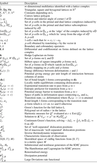
• versions of theDivergenceandStokes’ theoremswhich relate the above notions. Since these are likely to be familiar, we will point out some analogies with these more familiar calculus concepts along the way. The reader is invited to refer to Fig.1for an illustration of the particular lattice complexes used in the subsequent analysis.

2.1.1. Construction of a Lattice Complex Given a Hausdorff topological space S, a 0-cell is simply a member of some fixed subset of points in S. Higher-dimensional cells are then defined iteratively: for p 1, a p-dimensional cell (or p-cell) ise⊂Sfor which there exists a homeomorphism mapping the interior of the p-dimensional closed ball inRpontoe, and mapping the boundary of the ball onto a finite union of cells of dimension less than p.

Fig. 1. Thesquare,triangularandhexagonallattices respectively, and their duals. Primal lattices are shown ingrey, dual lattices inred; 2-cells areleft uncoloured. Particular primal cells are highlighted inblack, and their respective dual cells are given inblue(colour figure online)

Eachp-cell may be assigned an orientation consistent with the usual notion for set inRd_{, and we write−eto mean the p-cell with opposite orientation to that of} e. We may define an operator∂, called the boundary operator, which maps oriented p-cells to consistently oriented(p−1)-cells, which intuitively are ‘the boundary’ of the original cell. Similarly, the coboundary operatorδmay be defined, mapping an oriented p-cell,e, to all consistently orientedp+1-cells which haveeas part of their boundary.

We now recall from [4] that a lattice complex is a CW complex such that:

• the underlying space is all ofRd,

• the set of 0-cells forms and-dimensional lattice, and • the cell set is translation and symmetry invariant.

Throughout, we will denote such a lattice complexL, and the set ofp-cells of the corresponding complex will beLp. Due to the translation invariance ofL, it will be particularly convenient to consider translations of lattice p-cells, so fore∈Lp and a vectora∈Rd, we define

e+a:=x∈Rdx=y+a,y∈e.

We will always assume that we have chosen coordinates such that{0} ∈L0and, abusing notation, we will write 0 to refer to this 0-cell.

A second convenient notational convention we will occasionally use is the representation of a 1-cell through its boundary; we write

e= [e0,e1] to mean e∈L1 such that ∂e=e1∪ −e0.

2.1.2. Spaces of p-Forms and Calculus on Lattices For the application consid-ered here, we wish to describe deformations of a crystal. These are appropriately described in the lattice complex framework asp-forms, which are real-valued func-tions on p-cells which change sign if the orientation of the cell on which they are evaluated is reversed. We defineW(Lp)to be the space of allp-forms, that is

W(Lp):=

f :Lp→R f(e)= −f(−e), for anye∈Lp

It is straightforward to check that this is a vector space under pointwise addition. We also define the set ofcompactly-supported p-forms,

Wc(Lp):=

f ∈W(Lp)

{e| f(e)=0}is compact inRd

,

where here and throughout, Adenotes the closure ofA⊂Rd_. LetA⊂Lpbe finite; then for f ∈W(Lp), we define the integral

A

f := e∈A

f(e).

Thedifferentialandcodifferentialare respectively the linear operatorsd:W(Lp)→ W(Lp−1)andδ:W(Lp)→W(Lp+1), defined to be

df(e):=

∂e

f and δf(e):=

δe f.

For a 0-form on a lattice complex, the differential is simply the finite difference operator defined for a pair of nearest neighbours, and in a continuous setting the same operator is the gradient. Similary,δacting on 1-forms is either (the negative of) the discrete or continuum divergence operator. In a three-dimensional complex, bothd acting on 1-forms andδacting on 2-forms may be thought of as the curl operator.

The bilinear form

(f,g):=

Lp f g

is well-defined whenever f ∈Wc(Lp)org ∈Wc(Lp). Moreover, if f ∈Wc(Lp) andg∈Wc(Lp+1), we have the integration by parts formula

(df,g)=(f,δg); (2.1)

this statement should be compared with that of the Divergence Theorem and vari-ants, using the vector calculus interpretation ofdandδgiven above. Furthermore, by defining the spaceL2(Lp):=

f ∈W(Lp)(f, f) <+∞

, this bilinear form defines an inner product. It is straightforward to show that this is then a Hilbert space with the induced norm, which we denoteu2:=(u,u)1/2_.

We recall the definition of the Hodge Laplacian as the operator

:W(Lp)→W(Lp) with f :=(δd+dδ)f (2.2)

when p = 0 and p = m, and in the cases where p = 0 and p = m, = δd

and=dδrespectively. Note that, in a continuum setting, this definition of the Laplacian agrees with the interpretation ofdas the gradient on 0-forms andδas the negative of the divergence on 1-forms. Any function satisfyingf = 0 on

A⊂Lpis said to beharmonic on A. Finally,1ewill always denote thep-form

1e(e):=

2.2. Dual Complex

The common notion of duality which occurs in algebraic topology relating to CW complexes is that of thecohomology. This is usually presented as an abstract algebraic structure, since it is only this structure which is needed to deduce topolog-ical information about a CW complex. In some cases it may also be given a more concrete identification, which will be particularly important for the subsequent analysis.

Given anm-dimensional lattice complex, when possible, we define the dual complex as follows:

• For anye∈Lm, lete∗:=

exdx, the barycentre of seteinRd, and let

L∗₀:= {e∗|e∈Lm}.

• For a collection of elementarym-cells A∈Lm, let

A∗:= e∈A

e∗. (2.3)

• Now, iterate overp=m−1,m−2, . . . ,0: for eachp, lete∈Lp, and consider δe ∈ Lp₊1 as a sum of elementary p-cells. Find the corresponding cells in

L_m∗_−p−1. Definee∗∈L_m∗_−pto be the convex hull of(δe)∗with(δe)∗removed, assigninge∗the same orientation ase. ForA, a sum of elementary p-cells, we again defineA∗via (2.3).

We define boundary and coboundary operators on the dual lattice complex,∂∗and

δ∗_{, so that}

∂∗e∗=(δe)∗, and δ∗e∗=(∂e)∗. (2.4) By construction,∗ : Lp → L∗m−p defines an isomorphism of the additive group structure usually defined on lattice complexes (see Section 2.2 of [4]). The equalities stated in (2.4) may then be interpreted as the statement of the Poincaré duality theorem (see for example Section 3.3 of [28]), and the construction described above is succinctly represented in the following commutation diagram.

Lp₊1 Lp Lp₋1

L_m∗_−p−1 Lm∗−p L∗m−p+1

* * *

∂ ∂

δ∗ _δ∗

δ δ

∂∗ _∂∗

Since the differential and codifferential operators inherit features from the struc-ture of the CW complex on which p-forms are defined, we now show that simi-lar duality properties hold for the differential complexes on L andL∗. For any

f ∈W(Lp), we define f∗∈W(L∗m−p)via

Again, it may be checked that∗ :W(Lp)→W(L∗m−p)is an isomorphism; in fact,∗ defines an isometry of the spacesL2(Lp)andL2(L∗m−p). The differential, denoted

d∗:W(L∗_p)→ W(L∗_p−1), and codifferential, denotedδ∗:W(L∗_p−1)→W(L∗_p), are then

d∗f∗(e∗):=

∂∗e∗ f∗=

δe

f =δf(e),

and δ∗f∗(e∗):=

δ∗e∗ f∗=

∂e

f =df(e).

Again, this relationship is concisely expressed in the following diagram.

W(Lp₊1) W(Lp) W(Lp₋1)

W(L∗_m−p−1) W(Lm∗−p) W(L∗m−p+1)

* * *

d d

δ∗ _δ∗

δ δ

d∗ d∗

2.3. Examples: The Square, Triangular and Hexagonal Lattices

In the analysis which follows, we focus exclusively on 2-dimensional lattice complexes, and in particular the triangular, square and hexagonal lattices denoted

Tr,SqandHxrespectively. LetR4andR6be the rotation matrices

R4:=

0 −1

1 0

and R6:=

₁

2 −

√

3 2

√

3 2

1 2

.

For convenience, we definee1:=a1:=(1,0)T, and

ei :=Ri₄−1e1 fori ∈ {1,2,3,4}, and aj :=R₆j−1a1 for j ∈ {1, . . . ,6}.

The triangular, square and hexagonal lattices are defined to be

Tr:= [a1,a2] ·Z2, Sq:=Z2, and Hx:=

√

3R4Tr∪

√

3R4Tr+e1

;

the nearest neighbour directions inSqare thereforeei, andaiinTrorHx. We may define lattice complexes based on these sets (see Sects. 2.3.2 and 2.3.3 of [4] and [5]), and moreover

Tr∗= √₃3R4Hx+1₃(a2+a3),

Sq∗=Sq+1₂(e1+e2),

and Hx∗=√3R4Tr+

√

3

3 (a1+a2).

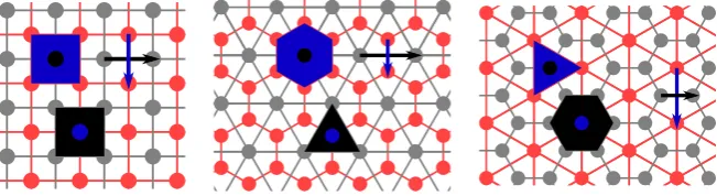
Fig. 2. On theleft, an example of primal (inblack) and dual (inred) induced subcomplexes for a general subset of thetriangularlattice:A0is the set ofblack points. On theright, a latticepolygonDin thesquarelattice, and the corresponding primal and dual subcomplexes, which are both path- and simply-connected (colour figure online)

At this point, we give the definitions of some lattice-dependent constants which will arise during our analysis:

K:=

⎧ ⎨ ⎩

3 ifL=Hx,

4 ifL=Sq,

6 ifL=Tr.

and V:=

⎧ ⎨ ⎩

2 ifL=Hx,

4 ifL=Sq,

6 ifL=Tr,

(2.5)

For convenience, we will writeV∗andK∗to mean the relevant constants for the dual lattice. Note thatKis the number of nearest neighbours in the lattice.

2.4. Finite Lattice Subcomplexes

For the particular application we will consider, we will make use of finite subcomplexes of the full lattice complex, and so we now make precise the notation we use as well as the particular assumptions made throughout our analysis. The reader may find it useful to refer to Fig.2, which illustrates the construction in a couple of simple cases.

2.4.1. Induced Subcomplexes Given a finite subsetA0 ⊂ L0, we define the induced lattice subcomplexby inductively defining

Ap:=

e∈Lp∂e⊂Ap−1

.

This is a well-defined CW complex when the corresponding boundary ∂A and coboundaryδAoperators are defined by restriction, i.e.

∂A_e:=∂e∩A

p−1, and δAe=(δe)∩Ap+1 for alle∈Ap.

It will be convenient to distinguish what we term theexterior andinterior p-cells of the CW complexA, respectively defined to be

Ext(Ap):= {e∈Ap|δe=δAe}, and Int(Ap):=Ap\Ext(Ap). The former set may be thought of as the ‘edge’ of the lattice subcomplex, and the latter as the ‘interior’ of the lattice subcomplex.

We now define a subcomplex of the dual lattice complex which we call thedual subcomplex induced byA0. LetA∗m := {e∗∈L∗m|e∈A0}, and inductively define

A∗_m−p:=e∗∈L∗_m−pe∗∈∂∗a∗for somea∗∈A_m∗_−p+1}

for p 1. We remark that this definition isnotequivalent to defining sets of sets of dual p-cells by directly taking the dual of the primal p-cells; however, we do have the inclusion

Ap

_∗

⊆A∗_m−p for eachp,

where equality always holds whenp=mby definition. The other inclusions follow by induction on p: note thate ∈ Apwith p 1 implies thate ∈ δAa for some a∈Ap−1,δAa ⊆δa, and hencee∗∈∂∗a∗for somea∗∈Am∗₋p₊1. As before, we may define∂A∗ andδA∗by restriction, which in turn leads us to define operators

dA∗andδA∗analogously. Similarly, let

Ext(A∗_p):=e∗∈A∗_pδ∗e∗=δD∗e∗, and Int(A∗_p):=A∗_p\Ext(A∗_p).

By construction, Ext(A∗₂)= ∅, ande ∈ Ext(A_n∗_−p)if and only if there exists no a∈Apwithe=a∗(see Fig.2for an illustration).

From now on, it will always be clear from the context whether we are referring to the relevant operators onLandL∗, or onAandA∗, so for the sake of concision, we will suppressAfrom our notation.

2.4.2. Subcomplexes Induced by a Domain We will say that an induced lattice subcomplex is path-connected if for anye,e∈A0, there existsγ ⊂A1such that

∂γ =e∪ −e,

and call suchγ ⊂A1apathwhich connectseande. We will say a lattice subcom-plex issimply-connectedif for anyγ ⊂A1such that∂γ = ∅,γ =∂Afor some

A∈A2.

Throughout our analysis,Dwill always denote a closed convex lattice polygon, i.e. a non-empty compact convex subset ofR2which has cornerscl ∈Land internal anglesϕlwherel=1, . . . ,Lindexes the corners, following [25]. We consider the scaled domainsnD, forn ∈N, noting thatnDremains a lattice polygon, and denote

Dnto be the largest induced lattice subcomplex with respect to inclusion such that • Dn,p⊂nDfor all p,

• D∗n_,p⊂nDfor all p,

• DnandD∗nare both path connected and simply connected.

2.4.3. Counting and Distances For a collection ofp-cells A⊂Dn_,p, we write #A to designate the smallest number of elementary p-cells ei such that A =

#A

i=1ei.

We define diam(D)to be

diam(D):=max|x−y|x,y∈D,

and we note that there exists a constantCL >0 which depends only on the under-lying latticeLsuch that

max

min#γγ ⊂Dn,1, ∂γ =e−e e,e∈Ext(Dn,0)

CLndiam(D).

We write dist(A,B)to mean the shortest distance between two sets A,B ⊂Rd, i.e.

dist(A,B):=inf|x−y|x ∈ A,y∈ B.

2.4.4. Spaces of p-Forms on Lattice Subcomplexes The space of p-forms on the lattice subcomplex induced bynDis denoted

W(Dn,p):=

u :Dn,p→Ru(e)= −u(−e)

.

As for the space of forms defined onL, we define the inner product and induced norm

(u, v):=

Dn,p

uv, and u2:=(u,u)1/2.

SinceDn,pis finite, these are always well-defined; we will also make occasional use of the norm

u∞:= max e_∈Dn,p

|u(e)|.

We denote the subspace of p-forms vanishing on Ext(Dn,p) W0(Dn,p):=

u∈W(Dn,p)u=0 on Ext(Dn,p)

,

which is clearly a vector space, and the bilinear form

((u, v)):=

Dn,1

dudv

is a well-defined inner product on W0(Dn,0).W0(Dn,0)is thus a Hilbert space with the corresponding norm, denotedu1_,2:=((u,u))1/2. We now demonstrate positive-definiteness of the inner product, since we will use the resulting version of Poincaré inequality below.

Since Dn is path-connected, for any e ∈ Int(Dn,0), there exists γ ⊂ Dn,1 such that∂γ =e∪ −e, withe ∈ Ext(Dn,0)and #γ C0Lndiam(D). For any u ∈ W0(Dn,0), we then haveu(e) =

γdu, so applying the Cauchy–Schwarz

inequality, we have

|u(e)|2=

γdu

2#γ

γ|du|

2_#γ

Integrating overDn_,0, and noting that there exists a constantC₁L >0 which depends only on the underlying latticeLsuch that #Dn,0C₁Ln2diam(D)2, we have

Dn,0 |u|2

C2Ln3diam(D)3

Dn,1

|du|2, (2.6)

whereC₂L=C₀LC₁L. We note that the same inequality also holds foru∈W0(D∗_n,0)

by a similar argument.

2.4.5. Duality for p-Forms on Lattice Subcomplexes We define the duality mapping∗ :W(nDn,p)→W0(D∗n_,2₋p)as follows:

u∗(a)=

u(e) a=e∗∈Int(D∗_n,2−p),

0 a∈Ext(D∗_n,2−p).

We note that this mapping is well-defined since as noted in Section2.4.1, a ∈ Ext(D∗_n,2−p) if and only if there exists no e ∈ Dp witha = e∗. This duality mapping defines an isomorphism fromW(Dn,p)toW0(D∗n−p)as vector spaces; as, in addition

(u,u)=

nDn,p |u|2₌

Int(nD∗n,p) |u∗|2₌

nD∗n,p

|u∗|2₌₍ u∗,u∗),

it follows that∗ defines an isometry of the spacesL2(nDn,p)toL2(D∗n,2−p). Moreover, for anye∈nDn,p, we verify that

du(e)=

∂e u=

(∂e)∗ u∗=

δ∗e∗

u∗=δ∗u∗(e∗), and

δu(e)=

δe u=

(δe)∗ u∗=

∂∗e∗

u∗=d∗u∗(e∗).

(2.7)

2.5. Dislocation Configurations

We now recall some definitions from [31] which will permit us to give a kinematic description of screw dislocations in the setting of our model. Given u ∈W(Dn,0), we define the associated set ofbond-length 1-forms

[du] :=α∈W(Dn,1)α∞ 1₂, α−du∈Z

.

Adislocation coreis any positively-oriented 2-celle∈D2such that

dα(e)=

∂eα= 0.

Letμ∈W(D2), withμ:D2→ {−1,0,+1}. We will say thatuis a deformation containing the dislocation configurationμif

The 2-form μrepresents theBurgers vectorsof the dislocations in the configu-ration, which are the topological ‘charge’ of dislocations; see [30,33] for general discussion of the notion of the Burgers vector and its importance in the study of dislocations, and [4,31] for further discussion of the physical interpretation of this specific definition.

For the purposes of our analysis, we define sets of admissible dislocation con-figurations. Forε >0,n ∈N, andbi ∈ {±1}fori =1, . . . ,m, we define the set Mε

n(b1, . . . ,bm)of 2-forms Mε

n(b1, . . . ,bm):=

μ=

m

i=1 bi1ei

ei∈D2positively oriented,dist(ei,Ext(Dn,0))nε,

dist(ei,ej)n,for alli,j∈ {1, . . . ,m},i= j

.

Each 2-form in this set represents a collection of mdislocations with respective Burgers vectorsb1, . . . ,bm and corese1, . . . ,em: these dislocations are separated from each other and from the boundary by a distance of at leastεn. Since we will assume that the number of dislocationsm, and the Burgers vectorsb1, . . . ,bm are fixed throughout, we will suppress the dependence on(b1, . . . ,bm)from now on.

3. Main Results

3.1. Energy and Equilibria

As stated in the introduction, we follow [1,2,4,31,32,41] and consider a nearest-neighbour anti-plane lattice model for the cylinder of crystal. Letψ :R→Rbe given byψ(x):= 1₂λdist(x,Z)2; we consider the energy difference functional

En(y; ˜y):=

Dn,1

ψ(dy)−ψ(dy˜).

This functional is a model for potential energy per unit length of a long cylindri-cal crystal, and pointsDn,0correspond to columns of atoms which are assumed to be periodic in the direction perpendicular to the plane considered. For further motivation of this model, we refer the reader to Section 1 of [1].

Following Definition 1 of [31], we will say thaty∈W(Dn,0)is alocally stable equilibriumif there exists >0 such that

En(y+u;y)0 wheneveru1_,2ε.

Due to the periodicity ofψ, we note that any locally stable equilibrium generates an entire family of equilibria: lettingz∈W(Dn,0)taking values inH+Zfor some H ∈R, if yis a locally stable equilibrium, then so isy+z. These equilibria are physically indistinguishable, since they correspond to a vertical ‘shifts’ of columns by an integer number of lattice spacings, and a rigid vertical translation of the entire crystal byH. We therefore define the equivalence relation

and denote the equivalence classes of this relation asy.

We recall that Theorem 3.3 in [31] gives sufficient conditions such that locally stable equilibra containing dislocations exist in the case of a more general choice ofψthan that chosen here. Our first main result is similar, but in addition provides a very precise representation of the corresponding bond-length 1-form in the case considered here, and asserts the uniqueness (up to lattice symmetries) of local equilibria containing a given dislocation configuration.

Theorem 3.1.Fixε >0andDa convex lattice polygon; then for all n sufficiently large, the following statements hold:

(1) For every2-formμ∈ Mnε, there exists a corresponding locally stable equi-librium u_μwhich contains the dislocation configurationμ;

(2) Each such equilibrium u_μis unique up to the equivalence relation defined in (3.1); and

(3) For any u ∈ u_μ, there is a unique bond-length1-formα ∈ [du]satisfying α∗_=d∗_{Gμ∗, whereμ}∗_{is the0-form dual toμ, and Gμ∗ ∈W0(D}

n,0)is the solution to

∗G_μ∗=μ∗inInt(D∗n_,0), with Gμ∗ =0onExt(D∗n_,0). (3.2)

Strategy of Proof The proof of this theorem is the main focus of Section4. We begin by showing that ifuis a locally stable equilibrium containing dislocations

μ, thenα∈ [du]must necessarily satisfy

α∞<12, dα=μonD2, and δα=0 onDn,0. (3.3)

We show that these conditions are satisfied by at most oneα∈W(Dn,1), and using the duality transformation described in Section2.2, we verify thatα ∈ W(Dn,1) satisfyingα∗ =d∗G_μ∗ verifies the latter two conditions. Showing thatα_∞ = d∗Gμ∗_∞ < 1₂ is the most technical aspect of the proof, and requires us to develop a theory which is analogous to obtaining interior estimates for solutions of a boundary value problem for Poisson’s equation in the continuum setting. To conclude, we obtain the classu_μby ‘integrating’α.

3.2. Energy Barriers

Let C[0,1];W(Dn_,0)

denote the space of continuous paths from [0,1]to W(Dn_,0). Forμandν ∈Mnε, we define the set of continuous paths which move any local equilibrium inuμto any other local equilibrium inuνto be

n(μ→ν):=

γ ∈C[0,1];W(Dn,0) γ (0)∈uμ, γ (1)∈uν, ∀t ∈ [0,1], α∈ [dγ (t)]impliesdα=μordα=ν.

configurations along the path vary only on the 2-cells pandq. In other words, we make the modelling assumption that dislocations move strictly from one site to an adjacent site, and not via a more complicated route.

We define theenergy barrier for the transition fromμtoνforμ, ν ∈M_nεto be

Bn(μ→ν):= min

γ∈n(μ→ν) max

t∈[0,1]En(γ (t);uμ). (3.4) Our second main result concerns an asymptotic representation of this quantity.

Theorem 3.2.Suppose thatμ, ν∈Mnεare2-forms such thatν−μ=bi[1q−1p] for some i , where q∗ = p∗+a∗for some nearest neighbour directiona∗inL∗. For i =1, . . . ,m, let xi ∈ Dbe such thatdist(xi,_n1e∗_i) _n1. Then there exist a constant c0which depends only on the underlying lattice complexLsuch that

Bn(μ→ν)=λc0+1₂λn−1

⎡

⎣b_i2∇ ¯yj(xj)·a∗+

i|i=j

bjbi∇Gxi(xj)·a

∗ ⎤

⎦₊o(n−1),

where

(1)λis given in the definition ofψ, (2) yj¯ solves the boundary value problem

y¯j =0inD, y¯j(·)= _V1_π log(| · −xj|)on∂D,

(3)Gy is the solution to

Gy = V₂δyinD, with Gy =0on∂D,

where we recall the definition ofV from(2.5), and

(4)o(n−1)satisfies no(n−1)→0as n→ ∞, uniformly for allμ∈M_nε.

Strategy of Proof The proof of this result is the main focus of Section5. Our main task is the explicit construction of atransition state, i.e.u_↓∈W(Dn,0)such that

En(u_↓;u_μ)= min

γ∈n(μ→ν) max t∈[0,1]En

γ (t);u_μ.

This may be seen as a generalisation of the notion of a critical point, but is not a true critical point, since Enis not differentiable atu_↓. Nevertheless, we show that

α ∈ [du_↓]has a dual which is closely related to the interpolation ofd∗G_μ∗and

d∗G_ν∗which are solutions of (3.2). This dual representation, combined with the precise asymptotics obtained ford∗G_μ∗in order to prove Theorem3.1, allow us to derive the expression ofBn(μ→ν).

3.3. Remarks on the Model

More General Potentials The derivation of the energy we consider as given in Section 2.2 of [2] suggests that potential ψ should be chosen to be smooth, in keeping with the usual assumptions on interatomic potentials. On the other hand, our results rely heavily on the definition ofψ, since the structure of the potential chosen permits us both to prove the characterisation and uniqueness ofαgiven in Theorem3.1, and to be precise about the set on whichB(μ→ν)is attained. This ultimately provides us with a means by which to prove Theorem3.2.

In spite of this, a result similar to Theorem3.2may hold in cases whereψis more general, but is sufficiently ‘close’ to the choice made here (see for example the structural assumptions made in Section 5 of [2]). Since the interatomic distances rapidly approach those predicted by linear elasticity as one moves away from a dislocation core (see Theorem 3.5 in [17]), and much of the potential energy is carried by the elastic field at significant distances from the dislocation core where a harmonic approximation of the energy is valid, heuristically one might expect that the energy barrier should be similar to that given in Theorem3.2. However, due to the complexity of possible transitions in a more general case, such a result does not seem tractable without very strong assumptions on the potential, and significant additional technicalities: we therefore do not pursue such results here.

Dynamics in the Infinite Lattice We remark that a significant amount of our analysis is devoted to verifying the first condition in (3.3) holds. This aspect of the proof of Theorem3.1would be significantly simplified if we were to consider the problem in an infinite domain, since in this case integral representations of the lattice Green’s function are available via Fourier-analysis. Nevertheless, we pursue the evolution on a finite domain here, both because this is a case of physical relevance, and because we are able to demonstrate that the boundary affects the evolution of the configuration in exactly the manner described in Section 2.1 of [46].

Equilibrium Conditions and Geometry Finally, we remark that the two latter conditions in (3.3) are analogous to the requirement that a continuum strain fieldε satisfies

curl(ε)=μ and div(C:ε)=0.

These are the conditions usually prescribed on a strain fieldεwhich contain dislo-cations described by a measureμin a linear elastic setting (see for example (1.1) in [14]).

We also note that the precise notion of duality which we use is specific to two-dimensional modelling of dislocations, as it is only in this case thatL1andL∗₁are related by duality. The fact that dual 1-cells are orthogonal segments suggest that one should view the construction ofαby duality as a version of the Cauchy–Riemann equations for harmonic conjugate functions.

3.4. KMC Model for Dislocation Motion

motion we wish to study. In doing so, we make several modeling assumptions, which we now discuss in detail.

Our first assumption is that the only possible transitions are fromμ∈ M_nεto

ν∈Mε

n satisfying

ν−μ=bi[1q−1p] for somei∈ {1, . . . ,m},

with p∗=q∗+a∗ for some dual lattice nearest-neighbour directiona∗.

This requirement prevents the following possible situations from arising:

(1) Multiple dislocations cannot move together in a coherent way: it seems reason-able to dismiss this possibility since we consider a regime where dislocations are far apart.

(2) Single dislocations cannot make successive correlated jumps over several lat-tice sites. Since we consider a low temperature regime, we expect the proba-bility of multiple correlated jumps to be negligible.

(3) Dislocations cannot be spontaneously generated in the material during the course of the evolution. In this case, we expect the energy barrier for dipole creation to be higher than that for the motion of single dislocations, so once again, we expect such events to be of very small probability and we therefore neglect them.

We therefore assume that the transition time for a dislocationμtoν is expo-nentially distributed with rate

Rn(μ→ν):=An(μ→ν)exp

−βBn(μ→ν)

, (1.1)

where:

(1) Bn(μ → ν)is the energy barrier for the transition fromμ toν defined by (3.4),

(2) β =(kBT)−1is the inverse thermodynamic temperature, and

(3) An(μ→ν)is the pre-exponential rate factor which is related to the entropic ‘width’ of the pathways connectingμandν, and hence also depends on the inverse temperatureβ.

for the original one-dimensional derivation, or [27] for an overview of variants derived in a variety of situations]

A(μ→ν)=

!

γ2_+4|λ

1(z)| −γ 2π

"

det∇2_V(x)

|det∇2_V(z)|+o(1). (3.5)

Hereγis a friction coefficient, with units of time−1, andλ1(z)is the eigenvalue of the Hessian atzwhich corresponds to the unstable direction. The rate can be reduced if either the eigenvalues of∇2V(x)are made smaller, reducing its determinant, or if the positive eigenvalues of∇2V(z)are increased. The former means the potential energy ‘basin’ aroundxis wider, and the latter means that the ‘mountain pass’ in the energy landscape through which the system can travel most easily to arrive at stateνis narrower. This coefficient therefore encodes entropic effects related to the shape of the energy landscape.

In our model, we have shown that there is a discontinuity in the first derivative at the energy barrier between states, so the exact expression (3.5) cannot be valid; however, in directions for which second derivatives exist, the Hessian of the energy at the transition state and at equilibria are identical, motivating the assumption that

Anis constant asn → ∞andβ → ∞. We remark that it is usual in practice (except in symmetric situations where multiple transition pathways with the same energy barrier exist) to choose a constant prefactor in KMC simulations, since eigenvalue decompositions of the Hessian of the energy are often unavailable, and transition events may be too rare to obtain a sufficiently accurate numerical estimate of the rate. In order to describe the limit, we define the set of admissible (macroscale) dislocation positions to be

M∞ε :=(x1, . . . ,xm)∈Dmxi∈D,|xi−xj|ε,dist(xi, ∂D)ε,∀i,jwithi= j,

and identifyM_nεwith a subset of this space by the embedding

ιn:Mnε →M∞ε, where ιn

m

i=1 bi1ei

=1

ne1∗, . . . ,1ne∗m

. (3.6)

It is clear that this map is well-defined, and by endowingM_nεwith the metric

rn(μ, ν)= m

i=1 1 ndist

e∗i, (ei)∗

where μ= m

i=1

bi1ei andν = m

i=1 bi1e_i,

andM_∞ε with the metric

r∞(μ, ν)=

m

i=1

dist(xi,xi) where μ=(x1, . . . ,xm)andν=(x1, . . . ,xm ),

Given a differentiable function f :M_∞ε → R, we will write∂if(x)to mean theR2-valued function such that

∂if(x)·a= f(x1, . . . ,xi+a, . . . ,xm)−f(x1, . . . ,xm)+o(|a|) for alla∈R2.

Let D([0,T];M_nε)denote the Skorokhod space of càdlàg maps from[0,T] ⊂

Rwith values inM_nε, and denote the space of continuous real-valued functions defined onM_nεto be C(M_nε;R): this is in fact the space of all real-valued functions onM_nε, since the metricrninduces the discrete topology. Define

Nμ:=ν∈Mnεrn(μ, ν)=dL

, where dL =

⎧ ⎨ ⎩

√

3

3 L=Tr, 1L=Sq,

√

3L=Hx.

Since we expect our modelling assumptions to break down as dislocations either approach one another or the domain boundary, we stop the evolution in such an event. We therefore denote what we term theboundary of M_nε, defined to be

∂Mε

n :=

μ= m

i=1

bi1ei ∈Mnε∃ν /∈Mnεsuch thatrn(μ, ν)=dL

#

.

We consider the sequence of Markov processesYn ∈ D[0,T];M_nεwhich are killed on the boundary∂Mnε, having infinitesimal generatorn : C

Mε

n;R

→ CMnε;R

where

[nf](μ):=

⎧ ⎨ ⎩

ν∈Nμ

TnRn(μ→ν)[f(ν)− f(μ)], μ∈Mnε\∂Mnε,

0 μ∈∂M_nε,

andRn(μ → ν)is defined in (1.1). SinceRn(μ → ν)is strictly positive and bounded for allμ, ν∈Mnεandn∈N,nis a bounded linear operator. Defining

Xnt :=ιn(Ytn), it follows thatXtnis a Markov process on the spaceM_∞ε.

3.5. The Feng–Kurtz Approach to Large Deviations Principles

The last of our main results will be to show that in a specific asymptotic regime, the Markov processesXnsatisfy a Large Deviations Principle. To do so, we apply the general theory developed in [21], which provides an approach to proving such results by demonstrating the convergence of a sequence of nonlinear semigroups. For convenience, we provide the following theorem as a synthesis of the results of Theorem 6.14 and Corollary 8.29 in [21], adapted to our application.

Theorem 3.3.Suppose that the following conditions hold:

(2)For all n∈N,(Mn,rn)is a complete separable metric space and there exists a sequenceιn:Mn→M of Borel measurable maps such that for any x ∈M, there exists zn∈Mnsatisfyingιn(zn)→x.

(3)For each n∈N,n:C(Mn;R)→C(Mn;R)is the infinitesimal generator of a Markov process on Mn. Suppose the martingale problem is well-posed, i.e. for any initial distributionμ0on Mn, the distribution of the Markov process at all later times is uniquely determined, and the mapping from y∈Mnto trajectories with initial distributionδyis Borel measurable under the weak topology on the space of probability measures defined onD([0,+∞);Mn).

(4)For any n∈N, and any f ∈C(Mn;R), define thenonlinear generator

Hnf(x):= 1_ne−n f(x)nen f

(x). (3.7)

Let H be an operator mappingC1(M;R)to the space of bounded measurable functions on M, which is represented as

H f(x)=Hx,∇f(x),

whereH:M ×RN →Rsatisfies the following conditions:

• His uniformly continuous on the interior of M×Br(0)for all r>0, • His differentiable in p on the interior of M×RN,

• H(x,p)=0for all p∈RN when x∈∂M, and • For all x ∈M, p→H(x,p)is a convex function.

For each pair(f,g)such that g= H f , there exists a sequence(fn,gn)such that gn = Hnfn,f ◦ιn− fn →0, gn is uniformly bounded, and for any sequence zn∈Mnsatisfyingιn(zn)→x, we have

gl(x)lim inf

n→∞ gn(zn)lim sup_n→∞ gn(zn)g u₍

x), (3.8)

where gland guare respectively the lower and upper-semicontinuous regular-izations of g,

gl(x):= lim r→0y_∈infBr(x)

g(y) and gu(x):= lim

r→0_y∈sup_Br(x)g(y).

(5)There existsL:M×RN→ [0,+∞]such that L(x, ξ)= sup

p∈RN

ξ·p−H(x,p),

lim

|ξ|→∞

L(x, ξ)

|ξ| = +∞ for all x∈ M andξ ∈RN, (3.9)

and for each x0∈ M, there exists x∈W1,1([0,T];RN)satisfying x(0)=x0

and

T

0

Then the sequence of M-valued processes Xn := ιn(Yn)with Xn(0) = ιn(yn), where yn ∈Mnandιn(yn)→x0as n → ∞, satisfy a Large Deviations Principle with rate functional

J(x):=

⎧ ⎨ ⎩

_∞

0

L(x,x˙)dt x∈W1,1[0,+∞);RNwith x(0)=x0,

+∞ otherwise.

(3.11)

Section6 contains the proof of this result, which amounts to checking that the assumptions above correspond to a series of conditions in [21].

3.6. Asymptotics for the KMC Model

An important condition of Theorem3.3is the verification of the convergence of the nonlinear generator,Hn. It will be this which motivates our particular choice of regime after we have non-dimensionalised the model. Since we are interested in the physically-relevant case of observing a large system over a long timescale, we let

Tn1 be the timescale of observation, which will be taken relative to the typical timescale on which a dislocation configuration changes. We then multiply all rates by this timescale, which we view as corresponding to observing the process over a long timescale.

Now, recalling the definition of the nonlinear generator given in (3.7), suppose that f ∈C1(M_∞ε;R), and and letxn=(1_ne∗₁, . . . ,1_ne_m∗). By Taylor expanding f, we find that

Hn(f ◦ιn)(xn)

= m

i=1

K∗

j=1

TnRn(μ→ν) n

exp∂i f(xn)·si,j+o(1)

−1 asn→ ∞,

wheresi,jare the nearest neighbour directions inL∗ate∗_i, andK∗is the number of nearest neighbours inL∗. Now, by applying Theorem3.2and the assumption that

An(μ→ν)=A0+o(1), we have that TnRn(μ→ν)

n =

TnA0e−βλc0

n exp

$

−βλ

2n∂iE(xn)·si,j

%

+oTn n

,

where E(x):= m

i=j

b2_jyj¯ (xj)− m

i,j=1 i<j

1

2bibjGxi(xj).

Here, following [2] we have defined therenormalised energy,E.−∂iE(x)is the Peach–Köhlerforce on the dislocation atxi, and hence the gradient flow dynamics ofEcorresponds to Discrete Dislocation Dynamics. We identify two parameters in this expression,

A:=TnA0e

−βλc0

n and B:=

βλ