Anthropogenic disturbance in tropical forests can double biodiversity loss from deforestation

(1)

Anthropogenic disturbance in tropical forests

can double biodiversity loss from deforestation

Article in Nature · June 2016 DOI: 10.1038/nature18326

CITATIONS

0

READS

929

28 authors, including:

Joice N. Ferreira

Brazilian Agricultural Research Corporation…

40PUBLICATIONS 441CITATIONS

SEE PROFILE

Ricardo Solar

Federal University of Minas Gerais

30PUBLICATIONS 185CITATIONS

SEE PROFILE

Ima Celia Guimarães Vieira

Museu Paraense Emilio Goeldi - MPEG

129PUBLICATIONS 2,708CITATIONS

SEE PROFILE

Carlos M. Souza

Amazon Institute of People and the Environ…

105PUBLICATIONS 3,471CITATIONS

SEE PROFILE

(2)

Anthropogenic disturbance in tropical forests

can double biodiversity loss from deforestation

Jos Barlow1,2,3_{, Gareth D. Lennox}1_{, Joice Ferreira}4_{, Erika Berenguer}1_{, Alexander C. Lees}2,5_{, Ralph Mac Nally}6_,

James R. Thomson6,7_{, Silvio Frosini de Barros Ferraz}8_{, Julio Louzada}3_{, Victor Hugo Fonseca Oliveira}3_{, Luke Parry}1,9_,

Ricardo Ribeiro de Castro Solar10_{, Ima C.G. Vieira}2_{, Luiz E. O. C. Arag˜ao}11,12_{, Rodrigo Anzolin Begotti}8_,

Rodrigo Fagundes Braga3_{, Thiago Moreira Cardoso}4_{, Raimundo Cosme de Oliveira Junior}4_{, Carlos M. Souza Jr}13_,

Nárgila G. Moura3_{, Sâmia Serra Nunes}13_{, João Victor Siqueira}13_{, Renata Pardini}14_{, Juliana Silveira}1,3_,

Fernando Z. Vaz-de-Mello15_{, Ruan Carlo Stulpen Veiga}16_{, Adriano Venturieri}4_{& Toby A. Gardner}17,18

Concerted political attention has focused on reduc-ing deforestation1−3_{, and this remains the cornerstone} of many biodiversity conservation strategies4−6_{. Yet} maintaining forest cover may not reduce anthropogenic forest disturbances, which are rarely considered in conservation programmes6_. _{These disturbances} oc-cur both within-forests, including selective logging and wildfires7,8_{, and at the landscape level, through edge,} area and isolation effects9_{. To date, the total combined} effect of anthropogenic disturbance on the conservation value of remnant primary forests is unknown, making it impossible to assess the relative importance of forest dis-turbance and forest loss. We address these knowledge gaps using an unparalleled data set of plants, birds, and dung beetles (1538, 460 and 156 species, respectively) sampled in 36 catchments in the Amazonian state of Pará. Catchments retaining>69-80% forest cover lost more conservation value from disturbance than from forest loss. For example, a 20% loss of primary for-est, the maximum level of deforestation allowed on Ama-zonian properties under Brazil’s Forest Code5_{, resulted} in a 39-54% loss of conservation value, 96-171% more than expected without considering disturbance effects. We extrapolated the disturbance-mediated loss of con-servation value throughout Pará, an area larger than South Africa covering 25% of the Brazilian Amazon. Al-though disturbed forests retained considerable conser-vation value compared to deforested areas, the toll of dis-turbance outside Pará’s strictly protected areas is equiv-alent to the loss of 92,000-139,000 km2_{of primary forest.} Even this lowest estimate is greater than the area defor-ested across the entire Brazilian Amazon between 2006 and 201510_{. Species distribution models showed that} landscape and within-forest disturbance both made sub-stantial contributions to biodiversity loss, with the great-est negative effects on species of high conservation and functional value. These results demonstrate an urgent need for policy interventions that go beyond the

mainte-nance of forest cover to safeguard the hyper-diversity of tropical forest ecosystems.

Protecting tropical forests is a fundamental pillar of many national and international strategies for conserving biodiversity4−6_{. Although improved regulatory and}

incen-tive measures have reduced deforestation rates in some trop-ical nations1,11,12_{, the conservation value of the world’s}

re-maining primary forests may be undermined by the addi-tional impacts of disturbance, which falls into two broad categories (see Methods). First, landscape disturbance re-sults from deforestation itself, with area, isolation and edge effects degrading the condition of the remaining forests9_.

Second, within-forest disturbance, such as wildfires and se-lective logging, induces marked changes in forest structure and species composition8,13_.

Although the biodiversity consequences of both forms of disturbance are well studied, previous research has over-whelmingly focused on identifying the isolated effects of specific types of disturbance14,15_{. Such studies provide an}

incomplete understanding of the total disturbance-mediated loss of conservation value arising from multiple interacting drivers16_{and are unable to quantify the extent to which}

re-ducing forest loss will succeed in protecting tropical for-est biodiversity. Addressing these knowledge gaps is vi-tal for informing forest management strategies in tropical nations, not least because withforest disturbance can in-crease even as deforestation rates fall7,12,17 _{and thus}

re-quires different policy interventions (Extended Data Table 1).

We estimated the combined effect of landscape and within-forest disturbance on biodiversity in primary forests and compared these impacts to the biodiversity loss ex-pected in deforested areas, offering the first such anal-ysis for anywhere in the world. Our study focused on two large (>10,000 km2) frontier regions of the

Brazil-ian Amazon: Paragominas and Santar´em, located in the state of Par´a (see Methods). Large- and small-stemmed plants, birds and dung beetles were sampled in 371 plots

1_{Lancaster Environment Centre, Lancaster University, LA1 4YQ, UK.}2_{MCTI/Museu Paraense Emlio Goeldi, CP 399, Bel´em, Par´a, 66040-170, Brazil.}3_{Universidade Federal}

de Lavras, Setor de Ecologia e Conservação. Lavras, Minas Gerais, CEP 37200-000, Brazil.4_{EMBRAPA Amazônia Oriental. Belém, Pará, 66095-100, Brazil.}5_{Cornell Lab}

of Ornithology, Cornell University, Ithaca, New York 14850 USA.6_{Institute for Applied Ecology, University of Canberra, Bruce, ACT 2617, Australia.}7_{Arthur Rylah Institute}

for Environmental Research, Department of Environment, Land, Water and Planning, 123 Brown Street, Heidelberg, Vic. 3084, Australia.8_{Universidade de Sao Paulo, Escola}

Superior de Agricultura ”Luiz de Queiroz”, Esalq/USP, Avenida Pádua Dias, 11, Sao Dimas, Piracicaba, SP, Brazil. 9_{Universidade Federal do Pará (UFPA), Núcleo de Altos}

Estudos Amazonicos (NAEA), Av. Perimetral, Numero 1 - Guamá, 66075-750, Belém - PA, Brazil1_{0 Universidade Federal de Viçosa, Departamento de Biologia Geral. Av.}

PH Rolfs s/n. Vic¸osa, Minas Gerais, 36570-900, Brazil.1_{1 Tropical Ecosystems and Environmental Sciences Group (TREES), Remote Sensing Division, National Institute for}

Space Research - INPE, Avenida dos Astronautas, 1.758, Jd. Granja, 12227-010, Sao Jose dos Campos, SP, Brazil.1_{2 College of Life and Environmental Sciences, University}

of Exeter, Exeter, EX4 4RJ, UK.1_{3 IMAZON, Rua Domingos Marreiros, 2020, 66060-160, Bel´em, PA, Brazil.}1_{4 Instituto de Biociencias, Universidade de Sao Paulo, Rua do}

Matao, Travessa 14, 101, 05508-090 Sao Paulo, Brazil.1_{5 Universidade Federal de Mato Grosso, Instituto de Biociencias, Departamento de Biologia e Zoologia. Av. Fernando}

Correa da Costa, 2367, Boa Esperanca 78060-900 - Cuiaba, MT. Brazil.1_{6 Universidade Federal Fluminense, Rua Miguel de Frias, 9, Icara´ı, 4220-900, Niteroi, RJ, Brazil.}1₇

Stockholm Environment Institute, Linn´egatan 87D, Box 24218, Stockholm, 104 51, Stockholm. Sweden1_{8 International Institute for Sustainability, Estrada Dona Castorina, 124,}

(3)

0.0 0.2 0.4 0.6 0.8 1.0

Conse

rv

ation

value

0.0 0.1 0.2 0.3 0.4

Absolute loss (CVD)

0.0 0.2 0.4 0.6

0.00 0.25 0.50 0.75 1.00 Primary forest cover

Propo

rtionate loss

a

b

[image:3.595.84.262.50.529.2]

c

Figure 1: The conservation status of primary forests. a,

Conservation value in Paragominas (circles) and Santar´em (triangles).b,Total loss of conservation value due to disturbance.c,Total loss of conservation value due to disturbance expressed as a proportion of the expected conservation value without disturbance. Dashed lines show expectations without disturbance. Grey lines show all regressions, with the black solid line showing the median response (see Methods). Values were standardized across study regions. There was no significant difference in conservation values between regions in the median response (F1;26=1.45,P=0.24, analysis of covariance (ANCOVA)).

in thirty-six study catchments distributed along a landscape deforestation gradient (0-94%) (Extended Data Fig. 1). Thirty-one catchments contained remnant primary forests. Within these catchments, we sampled 175 primary forest plots. Of these, 145 had visible evidence of within-forest disturbance (logging and/or fire). The remaining 30 had no evidence of within-forest disturbance and, being located in the largest remaining forest blocks, had minimal

land-0km 200km 400km

BE GU

RO

TA XI

MA

0.0 0.1 0.2

Loss of CV

38−57

92−137 135−178

20−33 13−23

106−151

0.0 0.2 0.4 0.6 0.8

PA TA GU XI BE RO

Loss of conser

v

ation v

alue

Forest loss Disturbance a

b

Figure 2: Conservation value deficit over large spatial scales. a,Proportionate loss of conservation value (CV) from disturbance in Pará (median estimate; see Methods). Areas of endemism (AoE) are: Belém (BE), Guiana (GU), Rondônia (RO), Tapajós (TA) and Xingu (XI). These do not include the island of Marajó (MA). Grey shading denotes strictly protected areas.b,Proportionate loss of CV in Pará (PA) and its AoEs from forest loss and disturbance (median estimate). Error bars show the range over all approaches to estimating conservation value (see Methods). Numbers show disturbance relative to forest loss (percentage range over approaches).

scape disturbance18,19 _{(see Methods). Irrespective of their}

disturbance history, these primary forest plots held consider-ably more forest species than all other major land-uses (Ex-tended Data Fig. 2).

[image:3.595.320.524.53.413.2]

(4)

0.5 1.0 1.5 2.0

25 50 75 100

Forest Cover

Relati

ve odds of

species detection 1.0

2.0 3.0 4.0

20 40 60 80 100

Forest Cover

0.5 1.0 1.5 2.0

40 60 80 100

0.5 1.0 1.5 2.0 2.5

40 60 80 100

● ● ● ● ● ● ● ● ● ● ● ● ● ● 0.3 0.6 0.9 1.2 1.5

−1.0 −0.5 0.0 0.5

Mean

range si

ze

of birds ● ● ● ● _● _●_● ● ● ● ● _● _●_● 0.3 0.6 0.9 1.2 1.5

−0.8 −0.4 0.0

● ● ● ● ● ● ● ● ● ● ● ● ● ● 0.3 0.6 0.9 1.2 1.5

−1.0 −0.5 0.0

● ● ● ●● ● ● ● ● ●● ● 0.3 0.6 0.9 1.2 1.5

−1.0 −0.5 0.0 0.5 1.0

0.4 0.5

ParagominasLandscape disturbanceSantarém ParagominasWithin-forest disturbanceSantarém

Disturbance sensitivity of response groups High

Low Low High Low High Low High

a b c d

Undegraded forest Undegraded forest

[image:4.595.87.507.49.328.2]

e f g h

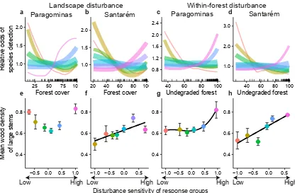
Figure 3: Response of forest birds to disturbance. a-d,The odds of detecting species groups along gradients of landscape (a, b) and within-forest (c, d) disturbance in Paragominas (a, c) and Santar´em (b, d) (see Methods). Species groups, shown by different coloured lines, are composed of species with similar disturbance responses (see Methods). Line thickness represents the relative size of the groups.e-h,Disturbance sensitivity of the species groups related to their mean range size (107_km2_{). Error bars shows s.e.m. Group colours correspond to groupings in}_a-d._{Black lines show significant}

relationships (P<0.05,F-test) (see Methods).

deficit (CVD). We take a variety of approaches to calculat-ing the CVD, reflectcalculat-ing different ways of classifycalculat-ing forest species, weighting their conservation value and calculating species density in undisturbed forest (see Methods). Here, we report median results from our sensitivity analysis along with the lower and upper bound range. Full results are shown in Figure 1 and Extended Data Figures 3 and 4.

The conservation value of the remaining primary forests was lower than expected along the entire deforestation gradi-ent. The CVD was unimodal with forest cover, reaching its maximum in catchments with 83% of their primary forests. These catchments retained just 58% of their conservation value (range: 48-65%) (Fig. 1a). The CVD was relatively small at low levels of forest cover (Fig. 1b). Yet disturbance caused the greatest proportionate loss of conservation value in these catchments, accounting for a c. 20-50% shortfall in the level of biodiversity that would be predicted for undis-turbed forests (Fig. 1c). The robustness of our estimates of the CVD was supported by the similarity of responses across study regions (Fig. 1) and sampled taxa (Extended Data Fig. 3).

The relationship we derived between forest cover and con-servation value allowed us, for the first time, to estimate the additional total impact of forest disturbance over large spatial scales. We therefore mapped the disturbance-induced loss of conservation value (CVD) across Par´a, which covers 1.26×

106_km2_{. We divided the state into grid cells approximately}

equal in area to our study catchments (c. 50 km2_).

Seventy-three percent of the c. 26,000 cells covering the state were

located in private lands or sustainable-use reserves. For these locations, which are most comparable to our study catch-ments, the total CVD was equivalent to c. 123,000 km2_of

forest loss (range: 92,000-139,000 km2_{). To put this figure in}

context, it is 51% (range: 38-57%) of the total area deforested across Par´a to date (Extended Data Table 2).

Our state-wide analysis revealed considerable spatial vari-ation in the CVD, reflecting differences in deforestvari-ation his-tories (Fig. 2a). We illustrate this variation by estimat-ing the additional loss of conservation value due to distur-bance across Par´a’s five major biogeographic zones (areas of endemism20_{, AoE). Median disturbance impacts outweighed}

biodiversity losses in deforested areas alone in three of the five AoEs (Fig. 2b). The high relative impact of disturbance is shown in the Guiana AoE, where the predicted loss of con-servation value from disturbance was 135-178% of the losses estimated in deforested areas. The relative impact of distur-bance was lowest in the Bel´em AoE, which has lost 62% of its native forest cover and is the most deforested AoE in Amazo-nia. Nonetheless, overall disturbance effects reduced Bel´em’s estimated conservation value from 38% when based on forest cover alone to just 26% (range: 24-30%).

(5)

1.0 1.5 2.0

25 50 75 100

Relati

ve odds of

species detection 1.0

1.5 2.0

20 40 60 80 100 0.8 1.2 1.6 2.0 2.4

40 60 80 100 1.0 2.0 3.0

40 60 80 100

● ●

●

● ●

●

0.4 0.6 0.8

−0.5 0.0 0.5

Mean

w

ood density

of large stems

● ●

●●

● ●

●

● ●

●●

● ●

●

0.4 0.6 0.8

−1.0 −0.5 0.0 0.5

● ● _● ● ●

●

● ● _● ● ●

●

0.4 0.6 0.8

−1.0 −0.5 0.0 0.5 1.0

● ● ●

●

● ●

● ● ●

●

● ●

0.4 0.6 0.8

−1.0 −0.5 0.0 0.5

1.0

Forest cover Forest cover Undegraded forest Undegraded forest

ParagominasLandscape disturbanceSantarém ParagominasWithin-forest disturbanceSantarém

High

Low Low High Low High Low High

a b c d

Disturbance sensitivity of response groups

[image:5.595.89.505.52.325.2]

e f g h

Figure 4: Response of large-stemmed plants to disturbance. a-d,The odds of detecting species groups along gradients of landscape (a, b) and within-forest (c, d) disturbance in Paragominas (a, c) and Santar´em (b, d) (see Methods). Species groups, shown by different coloured lines, are composed of species with similar disturbance responses (see Methods). Line thickness represents the relative size of the groups.e-h,Disturbance sensitivity of the species groups related to their mean wood density (g cm−3_{). Error bars shows s.e.m. Group colours correspond to groupings in}_a-d. _{Black lines show significant}

relationships (P<0.05,F-test) (see Methods).

within-forest disturbance (Extended Data Table 1)6,21_.

Here we provide insights into the need for additional poli-cies to reduce forest disturbance by examining the relative importance of landscape and within-forest disturbance on species distributions using Random Forests (see Methods). In ranking the importance of remotely-sensed disturbance mea-sures, we found that both forms of disturbance had significant additional effects on species’ distributions, albeit with some region- and taxon-specific variation (Extended Data Figs. 5-7, see Methods). We then used the measures of landscape and within-forest disturbance that were most frequently ranked highest to examine changes in taxon community structure, using Latent Trajectory Analysis to group species by their re-sponses to disturbance (see Methods). Results showed a con-sistent and high level of community turnover from both forms of disturbance, with some species groups responding nega-tively and others posinega-tively (Figs. 3 and 4, Extended Data Fig. 8). These responses may explain the unimodal shape of the disturbance impact (Fig. 1b) because they are consis-tent with the loss of highly sensitive species at relatively low levels of forest disturbance and the dominance of more re-sistant taxa in the most disturbed forests. Finally, we linked species’ response groups with life-history data available for birds and large-stemmed plants (see Methods). Both types of disturbance contributed to marked declines in species of high conservation and functional importance (birds with smaller range sizes22,23_{and plants with higher wood density}24−26_,

re-spectively) (Figs. 3 and 4). These analyses almost certainly underestimate the adverse effects of disturbance because rare species, which are often most sensitive to human impacts in forest ecosystems27_{, cannot be adequately modelled.}

We provide compelling evidence that Amazonian conser-vation initiatives must address forest disturbance as well as deforestation. At its most stringent, Brazil’s centrepiece forest legislation the Forest Code mandates Amazonian landowners to maintain 80% of their primary forest cover. Our results show that even in landscape that achieve this level of compliance, the remaining primary forests may only retain 46-61% of their potential conservation value and are likely to have lost many species of high conservation and functional importance. These findings reinforce the need to reduce the effects of landscape fragmentation by zoning development activities, thereby ensuring the protection of large blocks of remaining forest in all biogeographic zones. Where deforestation has already occurred, further conserva-tion losses can be minimised by preventing within-forest dis-turbance, aiding the recovery of already degraded forests, and investing in forest restoration to improve connectivity and buffer remnant forests from edge effects. Engendering change will require a mixture of incentive and regulatory-based measures to improve the sustainability of both forestry and farming practices. Crucially, because reducing forest disturbance requires coordinated efforts by many actors, in-terventions need to move beyond individual properties and address entire landscapes and regions. Such actions are ur-gently needed in the Amazon where logging operations are rapidly expanding across federal and state forests28_{, wildfires}

are increasingly prevalent during more frequent and severe dry seasons29_{, and the expansion of industrial agriculture,}

(6)

References

1. Boucher, D., Elias, P., Faires, J. & Smith, S. Deforestation Success Stories: Tropical Nations Where Forest Protec-tion and ReforestaProtec-tion Policies Have Worked. Union of Concerned Scientists June 2014 Report (2014).

2. Nepstad, D. et al. The end of deforestation in the Brazilian Amazon. Science 326, 13501351 (2009).

3. Soares-Filho, B. S. et al. Modelling conservation in the Amazon basin. Nature 440, 520523 (2006).

4. Convention on Biological Diversity. Strategic Plan for Biodiversity 20112020, Aichi Biodiversity Targets

https://www.cbd.int/default.shtml(2015).

5. Legislative Database of the Food and Agricultural Orga-nization of the United Nations (FAOLEX). Brazilian En-vironmental Law number 12.651 (25 March 2012). 6. Panfil, S. N. & Harvey, C. A. REDD+ and Biodiversity

Conservation: A review of the biodiversity goals, moni-toring methods and impacts of 80 REDD+ projects. Con-serv. Lett. 9, 143150 (2015).

7. Arag˜ao, L. E. O. C. & Shimabukuro, Y. E. The incidence of fire in Amazonian forests with implications for REDD. Science 328, 12751278 (2010).

8. Burivalova, Z., S¸ekercioglu, C. H. & Koh, L. P. Thresh-olds of logging intensity to maintain tropical forest biodi-versity. Curr. Biol. 24, 18931898 (2014).

9. Ewers, R. M. & Didham, R. K. Confounding factors in the detection of species responses to habitat fragmenta-tion. Biol. Rev. Camb. Philos. Soc. 81, 117142 (2006). 10. Instituto Nacional de Pesquisas Espaciais (INPE).

Pro-jeto Prodes: Amazon deforestation database. Avail-able at http://www.obt.inpe.br/prodes/index. php(2015).

11. Hansen, M. C. et al. High-resolution global maps of 21st-century forest cover change. Science 342, 850853 (2013). 12. Sloan, S. & Sayer, J. Forest Resources Assessment of 2015 shows positive global trends but forest loss and degradation persist in poor tropical countries. For. Ecol. Manage. 352, 134145 (2015).

13. Barlow, J. & Peres, C. A. Avifaunal responses to single and recurrent wildfires in Amazonian forests. Ecol. Appl. 14, 13581373 (2004).

14. Lewis, S. L., Edwards, D. P. & Galbraith, D. Increas-ing human dominance of tropical forests. Science 349, 827832 (2015).

15. Gibson, L. et al. Primary forests are irreplaceable for sus-taining tropical biodiversity. Nature 478, 378381 (2011). 16. Malhi, Y., Gardner, T. A., Goldsmith, G. R., Silman, M.

R. & Zelazowski, P. Tropical Forests in the Anthropocene. Annu. Rev. Environ. Resour. 39, 125159 (2014).

17. Morton, D. C., Le Page, Y., DeFries, R., Collatz, G. J. & Hurtt, G. C. Understorey fire frequency and the fate of burned forests in southern Amazonia. Phil. Trans. R. Soc. B 368, 18 (2013).

18. Gardner, T. A. et al. A social and ecological assessment of tropical land uses at multiple scales: the Sustainable Amazon Network. Phil. Tran. R. Soc. B 368, 20120166 (2013).

19. Berenguer, E. et al. A large-scale field assessment of carbon stocks in human-modified tropical forests. Glob. Chang. Biol. 20, 37133726 (2014).

20. da Silva, J. M. C., Rylands, A. B. & Da Fonseca, G. A. B. The fate of the Amazonian areas of endemism. Conserv. Biol. 19, 689694 (2005).

21. International Union of Forest Research Organizations (IUFRO). Understanding Relationships between Biodi-versity, Carbon, Forests and People: The Key to Achiev-ing REDD+ Objectives (eds Parrotta, J. A., Wildburger, C. & Mansourian, S.) (2012).

22. Manne, L. L., Brooks, T. M. & Pimm, S. L. Relative risk of extinction of passerine birds on continents and islands. Nature 399, 258261 (1999).

23. Purvis, A., Gittleman, J. L., Cowlishaw, G. & Mace, G. M. Predicting extinction risk in declining species. Proc. Biol. Sci. 267, 19471952 (2000).

24. Chave, J. et al. Towards a worldwide wood economics spectrum. Ecol. Lett. 12, 351366 (2009).

25. Phillips, O. L. et al. Drought sensitivity of the Amazon rainforest. Science 323, 13441347 (2009).

26. Baker, T. R. et al. Variation in wood density deter-mines spatial patterns in Amazonian forest biomass. Glob. Chang. Biol. 10, 545562 (2004).

27. Banks-Leite, C. et al. Assessing the utility of statistical adjustments for imperfect detection in tropical conserva-tion science. J. Appl. Ecol. 51, 849859 (2014).

28. Gestão de Florestas Públicas Relatório 2015. Bras´ılia: MMA/SFB Available athttp://www.florestal.gov.

br/publicacoes/instrumento-de-gestao(2015).

29. Chen, Y. et al. Forecasting fire season severity in South America using sea surface temperature anomalies. Sci-ence 334, 787791 (2011).

30. Ferreira, J. et al. Environment and Development. Brazils environmental leadership at risk. Science 346, 706707 (2014).

Acknowledgements This work was supported by grants from Brazil (CNPq 574008/2008-0, 458022/2013-6, and 400640/2012-0; Embrapa SEG:02.08.06.005.00; The Nature Conservancy Brasil; CAPES scholarships) the UK (Dar-win Initiative 17-023; NE/F01614X/1; NE/G000816/1; NE/ F015356/2; NE/l018123/1; NE/K016431/1), Formas 2013-1571, and Australian Research Council grant DP120100797. Institutional support was provided by the Herbrio IAN in Belm, LBA in Santarm and FAPEMAT. R.M. and J.R.T. were supported by Australian Research Council grant DP120100797. This is paper no. 49 in the Sustainable Ama-zon Network series.

Author Contributions T.A.G., J.F. and J.B. designed the research with additional input from E.B., A.C.L., S.F.B.F., J.L., V.H.F.O., L.P., R.R.C.S., I.C.G.V., L.E.O.C.A. and R.P. E.B., A.C.L., V.H.F.O., R.R.C.S, R.F.B., J.F., R.C.O., N.G.M. R.C.S.V., J.L., J.M.S and F.Z.V. collected the field data or analysed biological or soil samples. G.D.L. analysed the data, with input from J.B., J.R.T., R.M., A.C.L. and T.A.G. S.F.B.F., R.A.B., T.M.C., C.M.S., S.S.N., J.V.S., A.V. and T.A.G. processed the remote sensing data. J.B., G.D.L., J.F., A.C.L., R.M., J.R.T. and T.A.G. wrote the manuscript, with input from all authors.

(7)

Methods

Study regions. Par´a is the second largest state in Brazil and a focal point for deforestation, accounting for 34% of all forest loss in the Brazilian Amazon between 1988 and 201510_{. It holds exceptionally high biodiversity, with c. 10%}

of the world’s bird species and five of the eight major AoEs in Amazonia20_{. Within Par´a, we focused on two}

geograph-ically and biologgeograph-ically distinct regions: the municipalities of Paragominas and Santarém-Belterra-Moju´ı dos Campos (ab-breviated to Santarém) (Extended Data Fig. 1). These regions lie in different AoEs (Belém and Tapajós, respectively) and shared just 49% of our sampled taxa. Although they differ in their human colonization history18_{, both retain}_>_{50% of their}

native forest cover.

Study design and biodiversity sampling. We divided each region into third- or fourth-order drainage catchments. In each region, 18 study catchments (32-61 km2_{) were then distributed}

along forest cover gradients. We distributed study plots on

terra firmein proportion to forest and non-forest cover at a density of approximately 1 plot/4 km2_{, resulting in 8-12 plots}

separated by ≥1.5 km in each catchment (Extended Data

Fig. 1). Forest plots (n=234) were distributed without prior knowledge of anthropogenic disturbance18 _{and included}

pri-mary forests (i.e. under permanent forest cover;n=175) and

secondary forests recovering after agricultural abandonment (n=59). Non-forest plots (n=133) were predominantly

lo-cated in pastures (n=76) and mechanised agricultural lands

(n=31).

Thirty-one of the 36 catchments contained primary forest plots. In Paragominas and Santar´em respectively, these in-cluded undisturbed (13 and 17), logged (44 and 26), burned (0 and 7) and logged and burned primary forests (44 and 24)19_.

Disturbance categories were based on field assessments of fire scars, charcoal and logging debris, and an analysis of canopy disturbance, deforestation and regrowth in time series satel-lite images (1988 to 2010)18,19_{. Plots in the undisturbed forest} had no evidence of within-forest disturbance and, because they were located>2 km from edges in the largest forest blocks, had minimal landscape disturbance. Observations of hunting-sensitive large game birds, such as razor-billed curassowPauxi tuberosaand trumpetersPsophia spp.31,32_{, indicated low}

hunt-ing pressure33_{in undisturbed plots.}

Biodiversity surveys occurred during 2010 and 2011. The following descriptions apply to sampling at the plot level. Large and small stems: Live trees and palms with≥10 cm

diameter at breast height were identified in 10×250 m plots.

Smaller individuals (2-10 cm diameter) were sampled in five 5×20 m subplots (Extended Data Fig. 1). Liana diameters

were measured at 1.3 m from the main root. Large- and small-stemmed plants were analysed separately because they may differ in their disturbance responses. Individuals were identi-fied to species level by local parabotanists19_{. In total across}

all catchments, 175 plots and 825 subplots were sampled in primary forests. Birds: There were two repeat surveys of 15-min point counts at three sampling points (0, 150 and 300 m) (Extended Data Fig. 1). Sampling was undertaken between 15 minutes before dawn and 09:30. Lists of voucher sound-recordings and images are available for both regions31,32_{. In}

total across all catchments, 1050 point counts were undertaken in primary forests. Dung beetles: Sampled using pitfall traps (14 cm radius, 9 cm height) baited with 50 g of dung (80% pig and 20% human) and half filled with a killing solution (5%

detergent and 2% salt). Traps were left for 48 hours prior to inspection. Three traps were placed at the corners of a 3 m equilateral triangle, repeated at three sampling points (0, 150 and 300 m). In total across all catchments, 1575 pitfall traps were set in primary forests (Extended Data Fig. 1).

Defining the biodiversity consequences of forest loss, land-scape and within-forest disturbance.We limit the biodiver-sity consequences of forest loss to those that occur in defor-ested areas themselves, excluding any additional effects on remaining forests. Landscape disturbance then captures the combined edge, area and isolation effects that accompany the deforestation process. Within-forest disturbance refers to an-thropogenic disturbance events that are not inevitable conse-quences of forest loss or land cover change, including wild-fires, hunting and selective logging. Although often associ-ated with landscape factors, such as distance from forest edge, within-forest disturbance can occur independently of changes in forest cover or landscape configuration.

Estimating the conservation value deficit.We used the sum of forest species presences in primary forest plots to measure a catchment’s conservation value. In practice, this means that if a forest species occurs on xplots within a catchment, the species contributes xto the catchment’s conservation value. Total catchment conservation value is found by summing pres-ences over all forest species. This measure is equivalent to mean species richness (per unit area) in primary forests mul-tiplied by primary forest cover. In the absence of disturbance, conservation value should therefore respond linearly to for-est cover, with slope equal to mean species density,de. We

term the difference between this linear expectation and a catch-ment’s observed conservation value as its conservation value deficit (CVD). We took a variety of approaches to calculat-ing the CVD, reflectcalculat-ing different methods of defincalculat-ing forest species, weighting their importance, and calculatingde.

Defining forest species. We restricted our analysis to “forest species” to avoid attributing value to invasive and open-area species. We used three species classification filters: (i) an au-tomatic filter defined forest species as those that occurred at least once in a primary forest plot, irrespective of the plot’s disturbance history (n=1621 species); (ii) a high basal area (HBA) filter defined forest species to be those that occurred at least once in plots with a high average basal area (i.e. ≥the

lowest basal area recorded in undisturbed forests in each re-gion) (n=1290); and (iii) a convex hull filter where we first

applied a two-dimensional non-metric multidimensional scal-ing (MDS) to primary and secondary forest plots based on a stem-size classification (stress = 0.14), and then defined forest species to be those that occurred at least once in plots within the minimum convex hull of undisturbed primary forest plots on the MDS (n=1140).

(8)

There are many important life-history traits that correlate with species’ conservation or functional importance. Our choices were based on a priori knowledge and the availabil-ity of data for diverse tropical taxa. For birds we chose range size because it is the single most important predictor of threat status23_{, especially among lowland passerines where it is}

in-versely correlated with other important factors such as popu-lation density22_{. For plants we chose wood density because it}

is the most important size-independent determinant of carbon storage within individual stems, a strong predictor of carbon stocks across the biome24,26_{, and is also linked with other} func-tional properties24_{including drought resistance}25_{. Bird range}

sizes were extracted from the Birdlife Datazonehttp://www.

birdlife.org/datazone/index.html. Wood densities

were adapted from the global wood density database34_{, using}

the genus or family average where species or genus data were unavailable. Lianas were given a nominal value of 0.01.

As part of the broader sensitivity analysis we also undertook the same analysis described above for birds replacing species range size for species mean body size (body size data was also extracted from Birdlife Datazone). This analysis was under-taken to determine if the population density of birds, which is strongly and inversely correlated with body size, significantly affected results. It did not: the median estimate of the distur-bance impact decreased by just 0.5%, and we do not report the full results here.

Alternative undisturbed baselines. Estimating de (mean

species density in undisturbed landscapes) requires species distribution data from catchments with no within-forest or landscape disturbance. As we do not have a set of such catch-ments in either region, we took three approaches to calculat-ingde. The first two approaches rely on the least disturbed

catchment in each region. In both Paragominas and Santar´em, this reference catchment had minimal landscape disturbance (>99% primary forest). However, ground-based observations indicated that either selective logging or wildfire had affected at least 25% of the sampling plots within the reference catch-ments in both regions. We therefore calculateddeas the mean

species density over all plots in the reference catchment and, to correct for within-forest disturbance, as the mean density over only undisturbed reference catchment plots. Finally, to account for potential biases in underlying (natural) species dis-tributions, we also calculated de using all undisturbed plots

throughout each region (n=30). This represents a more con-servative estimate because it includes plots in catchments with less than 100% forest cover.

Selecting representative estimates of CVD.Combining the three forest species selection methods, the three species’ weighting approaches, and the three estimates of de returns

27 estimates of the CVD. For all approaches, we determined the average CVD with respect to primary forest cover by mod-elling the catchments’ summed presences with Poisson poly-nomial generalized linear models. We selected the best fitting model over all polynomials of degree up to cubics.

To express uncertainty over our estimates of the CVD, in the main text we present the median relationship between conser-vation value and forest cover along with the lower and upper bound range. We excluded from this range the estimate ofde

that included disturbed reference catchment plots, because it is not reflective of species density in the absence of disturbance. For the purposes of comparison, we have included these re-sults in Extended Data Figure 4. The median, lower and upper

bound estimates of the CVD were given by, respectively: the convex hull filter, linear species weighting, and undisturbed reference catchment plots; the convex hull filter, no species weighting, and all undisturbed plots; and the high basal area filter, exponential species weighting, and undisturbed refer-ence catchment plots.

Adjusting for proportionality.Although the number of plots in catchments was proportional to forest cover, proportional-ity was not exact because the original distribution was based on the extent of both primary and secondary forests18_{. We}

therefore corrected sampling effort by calculating the factor re-quired to make sampling proportional to primary forest cover in each catchment and scaled our estimates of conservation value accordingly. For each catchmenti, this factor is given bypi/ti, where piis the proportion of catchmentithat is

pri-mary forest andtiis the number of primary forest transects in catchmenti.

Extrapolating the CVD. To estimate disturbance impacts throughout Par´a, we divided the state into grid cells approxi-mately equal in size to our study catchments. We then used Brazil’s 2010 Terraclass product35 _{to determine the area of}

each cell that was deforested, first removing non-forested ar-eas that were covered by water or tropical savannah. We then calculated each cell’s conservation value by applying the me-dian, lower and upper bound estimates of the CVD. The distur-bance impact in forest loss equivalent terms for celliis given bypi−(ai−ni)vi, wherepi,ai,niandviare, respectively, the

cell’s primary forest extent, area, non-forest area and conser-vation value.

Linking landscape and within-forest disturbance with species distributions and traits. We investigated the impor-tance of landscape and within-forest disturbance at the plot level rather than the catchment level because many disturbance drivers act at local scales8,13_{. Variables representing landscape} and within-forest disturbance were based on the analysis of georeferenced 30 m resolution Landsat TM (Thematic Map-per) and eTM images from 1988 to 2010 in Paragominas and 1990 to 2010 in Santar´em. These were complemented by co-variates that represent natural variation in soil conditions, el-evation and slope. A full description of the data is available elsewhere18_{. Variable abbreviations match those in Extended}

Data Figs. 5-7.

Within-forest disturbance.We measured the cumulative extent of canopy disturbance36_{by calculating the percentage of the}

remaining primary forest in a 1 km buffer around each plot that had never been classified as disturbed (undisturbed pri-mary forest, UPF). We also included two measures of the fre-quency of disturbance within plots: the number of times the plot was logged (NL) and the number of times the plot was burnt (NB) in visual inspections of satellite images or field ob-servations.

Landscape disturbance. We used two landscape configura-tion measures: the density of forest-agriculture edges (ED) and the percentage of primary and secondary (>10 years old) forest cover (FC) in 1 km buffers around plots. We used two measures of landscape history37_{: the deforestation curvature}

profile (DC) and the land-use intensity profile (LI) in 500 m buffers around plots.

(9)

(pH), clay content (Cl), and carbon stock (Ca). We applied a 100 m buffer around each plot in a digital elevation model to calculate mean plot elevation (El) and slope (Sl).

Linking landscape and within-forest disturbance with species distributions and traits. We used Random Forests (RF), a decision-tree classification methodology, to identify species that are well-modelled by our data and to rank the importance of individual variables in accounting for species distributions. RF was adapted for spatial autocorrelation within catchments using a modified “residual autocorrelation” approach38_{. The fit of the RF models and their predictive}

performance was measured using area under receiver-operator curves (AUC)39_{. AUC evaluates the ability of models to}

cor-rectly predict higher probability of occurrence where species are present than where they are absent. An AUC value of 1 indicates perfect discrimination; a value of 0.5 suggests pre-dictions no better than random. We performed multiple cross-validations to evaluate model predictive performance. For each species, data from each study catchment were used in turn as test data for models built with data from the other catch-ments. The cross-validated AUC value, AUCcv, was calcu-lated as the average AUC value over all cross-validation tests for each species. Species present on a minimum of three tran-sects and with a summed AUCcv≥0.6 over all variables were classified as well-modelled and included in the analyses (31% of species). The importance of a variable was measured as its mean AUCcv over all well-modelled species.

Models included the within-forest disturbance, landscape disturbance and natural environment covariates described above. Given multicollinearity, we selected two variables from each group using three variable-selection methods: (i) we se-lected variables that we hypothesized to have the greatest influ-ence on species’ presinflu-ences (hypothesis driven selection); (ii) we used principal component analysis (PCA) on the full set of variables in each group and selected the highest loaded vari-able on the first two principal axes (PCA selection); and (iii) we ran RF on the full set of variables and selected the two highest ranked in each group (step-wise selection). Results for each method are shown in Extended Data Figs. 5-7.

Next, we used RF to determine species’ partial responses along disturbance gradients (Figs. 3 and 4 and Extended Data Fig. 8). These partial responses give the relative odds (exp(logit(p)−mean(logit(p)), wherepis the probability of species’ presence and logit is ln(p/(1−p)) of detecting each

species along a single variable gradient, holding all other vari-ables constant. For this analysis we selected the landscape and within-forest disturbance variables that were most frequently ranked highest in their group across the three variable selec-tion methods.

We then used latent trajectory analysis (LTA), which groups species’ partial responses into homogenous classes, to char-acterise the main types of response to the selected variables. We built models with up to eight classes and selected that with the lowest Bayesian Information Criterion (BIC) score. LTAs were carried out inRpackage “lcmm”http://cran.

r-project.org/web/packages/lcmm/lcmm.pdf. In

Fig-ures 3 and 4, we show the LOWESS smoothed response of

each species class along the associated disturbance gradient, with bandwidth set to 0.75.

Finally, we investigated the relationship between the distur-bance sensitivity of species classes, as determined by LTA, and species traits. To undertake this analysis, we defined a metric that represents the propensity of species classes to be detected along the variable gradients, which thus provides a measure of the sensitivity of the class to disturbance. The measure is:

hc(x) =Z u

m(x−m)dc(x)dx− Z m

l (m−x)dc(x)dx

wherem,landuare, respectively, the gradient’s mid-point and lower and upper bounds, anddc(x)is the relative odds of

detecting species classcat pointxon the gradient, as deter-mined by RF. We scaledhcto lie between±1. Values ofhc

close to 1 indicate that species classcis much more likely to be detected at the maximum than minimum extreme of the gra-dient, values close to−1 indicate that species classcis much

more likely to be found at the minimum than maximum ex-treme. Values near 0 indicate that species classcis equally likely to be detected at either extreme. We tested the relation-ship betweenhcand species’ traits by fitting polynomial

mod-els weighted by group size. In all cases, the response variable was the average value of the species trait over all species in each class. We investigated polynomial fits up to cubics and selected that with the lowest BIC score.

References

31. Lees, A. C. et al. One hundred and thirty-five years of avi-faunal surveys around Santarem, central Brazilian Amazon. Rev. Bras. Ornitol. 21, 1657 (2013).

32. Lees, A. C. et al. Paragominas: a quantitative baseline in-ventory of an eastern Amazonian avifauna. Rev. Bras. Or-nitol. 20, 93118 (2012).

33. Barrio, J. Hunting pressure on cracids (Cracidae: Aves) in forest concessions in Peru. Rev. Peru. Biol. 18, 225230 (2011).

34. Zanne A. E. et al. Data from: Towards a worldwide wood economics spectrum. Dryad Digital Repository. http:

//dx.doi.org/10.5061/dryad.234(2009).

35. Instituto Nacional de Pesquisas Espaciais (INPE). Terra-class data 2010; available athttp://www.Inpe.Br/cra/

projetos_pesquisas/terraclass2010(2013).

36. Souza, C. M. Jr. et al. Ten-year landsat classification of de-forestation and forest degradation in the Brazilian Amazon. Remote Sens. 5, 54935513 (2013).

37. Ferraz, S. F. D., Vettorazzi, C. A. & Theobald, D. M. Using indicators of deforestation and land-use dynamics to sup-port conservation strategies: A case study of central Ron-donia, Brazil. For. Ecol. Manage. 257, 15861595 (2009). 38. Crase, B., Liedloff, A. C. & Wintle, B. A. A new method

for dealing with residual spatial autocorrelation in species distribution models. Ecography 35, 879888 (2012). 39. Pearce, J. & Ferrier, S. Evaluating the predictive

(10)

0km 200km 400km

0km 30km 60km

Non−forest area Primary forest Secondary forest Water

0km 30km 60km

0km 3km 6km

Bird & beetle sampling point Small stem sampling Large stem sampling

10 m

0 50 100 150 200 250 300 m 20 m

5 m

a

b

c

d

e

(11)

Large stems Small stems Birds Beetles

● ● ● ● ● ● ● ●

● ●

● ●●●●●● ●_●●●

● ●

●

● ●

0.0 0.5 1.0 1.5

● ● ● ● ● ● ● ●

● ● ●

● ● ● ● ●

● ●

●

● ●

0.0 0.5 1.0 1.5

Relative species richness

● ● ● ● ● ● ● ●

● ● ●

● ● ● ● ● ● ● ● _●

● ● ● ●

● ●

●

● ●

0.0 0.5 1.0 1.5

SF PA AG SF PA AG SF PA AG SF PA AG

a

b

c

(12)

0.0 0.2 0.4 0.6 0.8 1.0

Conse

rv

ation

value

Large stems

Small stems

0.0 0.2 0.4 0.6 0.8 1.0

Conse

rv

ation

value

Birds

Beetles

a b

c d

Extended Data Figure 3: Conservation value of primary forests measured by individual taxa. a-d,Estimates of conservation value in the Paragominas (circles) and Santar´em (triangles) study regions from large-stemmed plants (a) small-stemmed plants (b) birds (c) and dung beetles (d). Dashed lines show expectations without disturbance. Grey lines show all regressions, with the black solid line showing the median response (see Methods). Values were standardized across study regions and taxa. There was no significant difference between taxa in the median estimate (F3;117=1.36,P=0.26,

(13)

0.0

0.2

0.4

0.6

0.8

1.0

0.00

0.25

0.50

0.75

1.00 Primary forest cover

Conse

rv

ation

value

Extended Data Figure 4: Range of conservation value estimates using three alternative sets of reference plots.Mean species density (de) is measured by: all disturbed and undisturbed plots in the least disturbed reference catchments (grey

(14)

● ● ● ● ●● ● ●

A

B

ED PFD UPF Sl FC Cl

0.00 0.25 0.50 0.75 AUCcv ● ● ● ● ●● ●

A

AB

C

Sl ED PFD UPF Cl FC

0.0 0.2 0.4 0.6 AUCcv ● ● ● ●●● ● ● ● ● ● ● ● ● ● ● ● ● ● ●●● ●

A

B

ED Sl UPF Cl PFD FC

0.00 0.25 0.50 0.75

● ● ● ● ●● ● ●●●●● ●● ●● ● ● ●● ●● ●● ● ● ● ●

A

AB

B

PFD ED Cl UPF FC Sl

0.00 0.25 0.50 0.75 ● ● ● ● ● ●●● ● ●●● ● ● ●●● ●●●● ● ●● ●● ● ● ● ● ● ● ● ● ● ●●

● ● ●

B

● ●

A

B

C

Sl ED Cl PFD UPF FC

0.00 0.25 0.50 0.75 1.00

● ● ● ●● ●● ●● ● ● ● ●● ● ● ● ●● ●● ●●● ●●● ● ● ●● ●● ●● ● ● ● ●

A

●

AB

BC

C

PFD ED UPF FC Sl Cl

0.00 0.25 0.50 0.75 1.00 ● ●● ● ● ● ● ● ●● ●●● ● ● ●● ● ● ● ● ● ●

A

B

BC

C

ED Sl Cl PFD UPF FC

0.00 0.25 0.50 0.75

● ●● ●● ● ● ● ● ● ● ●● ● ● ● ●●●● ● ● ●● ● ●

A

AB

BC

CD

D

ED PFD FC UPF Sl Cl

0.00 0.25 0.50 0.75

a

b

c

d

e

f

g

h

Extended Data Figure 5: The importance of hypothesis selected variable. a-h,Species AUCCVvalues for each variable

in Paragominas (a, c, e, g) and Santar´em (b, d, f, h) for large-stemmed plants (a, b), small-stemmed plants (c, d), birds (e, f) and beetles (g, h). Variable importance was measured by the mean AUCCVover all well-modelled species (see Methods).

Variable colours denote group membership: green, orange and blue represent landscape disturbance, within-forest

(15)

● ● ● ● ● ● ● ●

A

AB

B

ED PFD UPF FC El Cl

0.00 0.25 0.50 0.75 AUCcv ● ●● ● ● ● ●

A

AB

B

Cl El ED UPF PFD FC

0.0 0.2 0.4 0.6

AUCcv ● ● ● ● ● ● ● ● ● ●● ● ● ● ● ● ● ● ●●

A

AB

BC

C

ED El UPF Cl PFD FC

0.00 0.25 0.50 0.75

●●● ●●● ● ● ● ●● ●● ● ● ● ●●● ● ● ● ● ● ●

A

AB

BC

C

ED PFD Cl UPF FC El

0.00 0.25 0.50 0.75

● ●● ● ● ● ●●● ● ● ● ● ●●●●●● ● ● ● ● ●●● ● ● ● ● ● ● ●● ● ● ● ● ●●●●● ●

A

B

BC

C

ED Cl El UPF PFD FC

0.00 0.25 0.50 0.75

● ● ●● ●●● ●●● ●● ● ● ● ● ● ● ● ●●●● ● ● ● ● ● ● ●●● ● ● ● ●● ● ●●

A

AB

C

PFD ED UPF Cl FC El

0.00 0.25 0.50 0.75 1.00

● ● ●●● ● ●● ● ● ● ● ● ● ● ● ● ● ●● ●

A

B

CB

C

ED Cl El PFD UPF FC

0.0 0.2 0.4 0.6 0.8

● ● ● ● ●● ●● ●●● ● ● ●

A

AB

BC

C

ED PFD FC UPF Cl El

0.00 0.25 0.50 0.75 1.00

BC

a

b

c

d

e

f

g

h

Extended Data Figure 6: The importance of PCA selected variable. a-h,Species AUCCVvalues for each variable in

Paragominas (a, c, e, g) and Santar´em (b, d, f, h) for large-stemmed plants (a, b), small-stemmed plants (c, d), birds (e, f) and beetles (g, h). Variable importance was measured by the mean AUCCVover all well-modelled species (see Methods).

(16)

● ● ● ● ● ● ● ● ● ●

A

AB

B

ED NL UPF FC El Cl

0.00 0.25 0.50 0.75

AUCcv ● ● ● ● ●

A

ED Cl PFD UPF Ca FC

0.0 0.2 0.4 0.6

AUCcv ●● ● ● ● ● ● ● ● ●● ● ● ● ● ● ●

A

B

BC

C

El DC Cl UPF PFD FC

0.00 0.25 0.50 0.75 1.00

●● ●● ● ● ● ● ●● ●●● ● ● ● ● ● ● ● ● ● ●●● ● ● ● ●

A

AB

B

PFD DC Sl UPF FC El

0.00 0.25 0.50 0.75

● ● ●● ● ● ● ● ● ● ● ● ● ●●● ● ●● ● ●● ● ●●●● ●● ● ● ● ● ●●● ●● ● ● ● ●● ● ● ●●●●

●●

A

B

BC

CD

D

Ca DC Cl PFD UPF FC

0.0 0.3 0.6 0.9

● ● ● ●●●● ● ● ● ● ●●●● ●●●● ● ● ● ●● ● ● ● ● ● ● ● ●● ●

A

B

BC

C

ED UPF PDF FC Sl El

0.00 0.25 0.50 0.75 1.00

● ● ● ●●● ● ●● ●● ● ● ● ● ● ●● ● ●● ●

A

B

Ca DC PFD Cl UPF FC

0.0 0.2 0.4 0.6 0.8

● ● ●●● ● ●● ● ● ● ● ● ● ● ● ●●●● ● ● ● ●● ●

A

B

ED UPF NB FC Sl El

0.00 0.25 0.50 0.75 1.00

a

b

c

d

e

f

g

h

Extended Data Figure 7: The importance of step-wise selected variable. a-h,Species AUCCVvalues for each variable

in Paragominas (a, c, e, g) and Santar´em (b, d, f, h) for large-stemmed plants (a, b), small-stemmed plants (c, d), birds (e, f) and beetles (g, h). Variable importance was measured by the mean AUCCVover all well-modelled species (see Methods).

(17)

0.5 1.0 1.5 2.0 2.5

1.0 2.0 3.0

0.5 1.0 1.5 2.0

0.5 1.0 1.5 2.0 2.5 3.0

0.5 1.0 1.5 2.0

25 50 75 100 Forest cover

Relati

ve odds of species detection

0.6 1.0 1.4

20 40 60 80 100 Forest cover

1.0 1.5

40 60 80 100 Undegraded forest

0.5 1.0 1.5 2.0 2.5

40 60 80 100 Undegraded forest

Paragominas

Santarém

Paragominas

Santarém

Landscape disturbance

Within-forest disturbance

a

b

c

d

e

f

g

h

(18)

Extended Data Table 1: Policy interventions used to reduce deforestation and their effect on disturbance.

Extended Data Table 1

Policy intervention

Direct effects on reducing

land-scape disturbance

Direct effects on reducing

within-forest disturbance

Protected areas (IUCN classes

I-IV)

Positive if there is no leakage of

deforestation

Positive if park management is

effective and leakage of logging

is avoided

Sustainable-use reserves

(IUCN class VI)

Positive if there is no leakage of

deforestation

Positive where more sustainable

approaches replace conventional

approaches, and if leakage of

logging is avoided

Negative if forest-use is

incen-tivised in areas that would not

otherwise be disturbed

Legal stipulation to maintain

forest cover on private lands

Positive, but there is no stip-

ulation to consider landscape

configuration

No likely impact without

addi-tional measures

Agricultural intensification on

deforested lands

Positive if this prevents further

forest loss

Negative if increased profits

en-courage further land-use change

Negative if the matrix becomes

more hostile to forest species,

increasing isolation

Positive if reduced fire use in

agriculture prevents wildfires

No likely impact on selective

logging or hunting

Negative if there are new

spillover effects from

agricul-ture, such as deposition of

nutri-ents and pesticides

Industrial and community

based reduced impact logging

Positive if economic returns

protect forests from clearance

Negative when new roads and

logging patios increase

edge-effects and isolation

Positive if more sustainable

approaches replace conventional

logging

Negative when logging is

incen-tivised in undisturbed forests

Protecting forests through

moratoria & certification

Positive if this prevents further

forest loss and there is no

leak-age of deforestation

(19)

Extended Data Table 2: Forest loss and disturbance in Par´a and its areas of endemism. a-c,The loss of primary forest conservation value from forest loss and forest disturbance in forest loss-equivalent terms across c. 50 km2_{cells covering all}

land in Par´a (a), private lands and sustainable use reserves only (b), and private lands only (c). Disturbance losses are calculated using the median estimate of conservation value with the lower and upper bound range in parentheses (see Methods).Areais the total area of the region in km2_._{Forest area}_{gives the area of the region that was or is primary forest}

cover in km2_._{Forest loss}_{gives the total loss of primary forest in km}2_._Disturbance_{gives the loss of conservation value due}

to disturbance in km2_._Relative_{gives the disturbance-mediated loss of conservation value relative to that from forest loss.}